


Abstract
The majority of hydrogen in the interstellar medium (ISM) is in atomic form. The transition from atoms to molecules and, in particular, the formation of the H2 molecule, is a key step in cosmic structure formation en route to stars. Quantifying H2 formation in space is difficult, due to the confusion in the emission of atomic hydrogen (H i) and the lack of a H2 signal from the cold ISM. Here we present the discovery of a rare, isolated dark cloud currently undergoing H2 formation, as evidenced by a prominent "ring" of H i self-absorption. Through a combined analysis of H i narrow self-absorption, CO emission, dust emission, and extinction, we directly measured, for the first time, the [H i]/[H2] abundance varying from 2% to 0.2%, within one region. These measured H i abundances are orders of magnitude higher than usually assumed initial conditions for protoplanetary disk models. None of the fast cloud formation model could produce such low atomic hydrogen abundance. We derived a cloud formation timescale of ∼6 × 10⁶ years, consistent with the global Galactic star formation rate, and favoring the classical star formation picture over fast star formation models. Our measurements also help constrain the H2 formation rate, under various ISM conditions.
Export citation and abstract BibTeX RIS
1. Introduction
The formation of the H2 molecules is a key process in converting atoms into molecules in the interstellar medium and is the critical step in the formation of stars. Spitzer (1946) suggested that H2 formation occurs on dust grains, rather than in the gas phase, because the collision frequency is too low to provide sufficient three-body collisions in molecular clouds (Kaiser 2002). A widely accepted description of an efficient H i–H2 transformation process in clouds is provided by Hollenbach & Salpeter (1971). Efficient H2 formation can persist to high temperatures because chemisorbed atoms can stay on the grain surface while maintaining quantum mobility. Such configuration is conducive to hydrogen recombination (H2 formation) until the dust grain surface temperature reaches ∼500 K (Cazaux & Tielens 2004). Laboratory experiments demonstrated that H2 formation could also occur on carbon surfaces with a high recombination efficiency over a broad range of temperature (Vidali et al. 2005). The theoretical work in Cazaux et al. (2005) explained the high efficiency under low temperatures in both quiescent diffuse and dense clouds in terms of physisorption forces and thermally activated diffusion. Since the timescale of star formation is tightly constrained by the timescale of molecular gas formation, it is crucial to have a self-consistent understanding of the global star formation efficiency and star formation rate in galaxies. The timescale of star formation is controversial. The canonical model (Shu 1977) favored it to be around 10 Myr, while Bergin et al. (2004) and Elmegreen (2000), hypothesized that star formation occurs on a turbulent crossing scale that corresponds to about only 1 Myr on parsec scales (Glover & Mac Low 2007).
Direct measurement of H2 formation is difficult because H i is hard to isolate in the Galaxy and H2 lacks a permanent dipole moment, making it rare to have both measurements of H i and H2 gas for the same regions of the Galaxy. Key physical parameters need largely to be assumed in calculating cloud formation. Molecular hydrogen can be observed through absorption if it is against a good X-ray and/or ultraviolet background source (e.g., Sembach et al. 2001). Since H2 itself does not emit at the temperature of molecular clouds, these regions are generally traced emission from the lower rotational transitions of CO. However, subthermal excitation in diffuse gas and depletion in dense gas make CO unsatisfactory to trace H2 (Kramer et al. 1999). It is also difficult to probe the cloud formation timescale through astrochemistry based on molecular species other than H2 and H i, such as N2H+ and deuterated species (Caselli et al. 2002), because these tracers comprise only a tiny fraction of cloud mass. The foremost chemical reaction in molecular formation is the formation of molecular hydrogen. It is thus paramount for us to obtain direct measurement of the H2 formation timescale in order to better understand cloud formation timescale, the star formation efficiency and the star formation rate.
We have developed an observational method called H i Narrow Self-Absorption (H iNSA; Li & Goldsmith 2003; Goldsmith & Li 2005), which is capable of measuring atomic hydrogen abundance in dense clouds. Similar to the well-known H i Self-Absorption (H iSA (Heeschen 1955)) phenomenon in the cold neutral medium (CNM), H iNSA differs in a significant aspect, namely, the thermalization of H i at low temperatures through collisions with H2. Due to efficient cooling by molecular emission lines, especially the rotational transitions of CO, molecular clouds claim most of the lowest temperatures found in the Milky Way except for a few rare cases, such as those discussed by Knee & Brunt (2001) and Peek et al. (2011b). In contrast, lacking molecular cooling, H iSA is likely a result of temperature fluctuations in the CNM (Gibson et al. 2000). Systematic surveys have shown that H iNSA is associated with molecular clouds (Krčo & Goldsmith 2010), and thus provides a direct measurement of cold H i in dark clouds.
The left image in Figure 2 gives a schematic diagram of the transition from CNM to dense molecular gas. In the warm ionized medium and H ii regions, hydrogen is largely in the form of H+. For higher densities and lower UV intensities, H+ combines with electrons through radiative recombination and forms H i. With increasing H i volume density, hydrogen atoms start to form molecular hydrogen on the surface of dust grains. In diffuse molecular clouds, even when most of the H is in the molecular form, gas-phase carbon can still be mainly C+. After combining with H2 through radiative association, C+ becomes  ;
;  reacts rapidly with electrons to form CH; then CH reacts with O to produce CO. C+ can also react with electrons to form C i through dielectronic recombination. C i, along with OH, lead to the formation of CO through neutral–neutral reactions in colder (10 K < T < 100 K) dark clouds (Woodall et al. 2007). Other molecules form following CO in dense cores. In particular, N2H+, NH3, and cations like H2D+ become significant and have been used to study the cloud core formation timescale (Brünken et al. 2014).
Isolated, cold dark clouds are the ideal laboratory for studying H2 formation in the Milky Way. In a previous study, B227, CB45, and L1574, were identified as isolated dark clouds, and coincidently aligned in a linear configuration from north to south spanning about two degrees (Martin & Barrett 1978). There are no nearby UV sources such as massive stars or H ii regions.
In this paper, we present a combined analysis of H iNSA, CO emission, dust emission, and extinction for a rare, isolated dark cloud, currently undergoing H2 formation. The [H i]/[H2] abundance varies from 2% to 0.2%, within one region and the formation timescale was derived as ∼6 Myr, which is consistent with both an analytical model and a numerical chemistry model.
2. Observations and Data Reduction
To reconstruct the chemical state and the evolutionary history of isolated dark clouds, we mapped H i, 13CO J = 1–0 emission, and dust continuum emission in B227, CB45, and L1574, which were identified as H iNSA sources by Goldsmith & Li (2005). In 2012 May and November, the sources were observed in the 1420 MHz transition of H i using the Arecibo L-band Feed Array (ALFA) on the 305 m radio telescope. We implemented the observations in the "total power" mode because of a clear "off" position that was difficult to find in the Galaxy. The nominal system temperature of 30 K has contributions from the system temperature and the H i emission. In addition, the temperature of the H i emission from standard CNM is around 70 K (Heiles & Troland 2003). Hence, we consider an equivalent system temperature of 100 K for evaluating the observing sensitivity. To accomplish the mapping for the sources that extend 1° × 2°, the"leap frog" drift scan was adopted (Minchin et al. 2007). Spectra were recorded by GALSPECT, the Galactic ALFA spectrometer. The resolution is 0.18 km s−1 per channel with 7,679 channels. Using the Spectral and Photometric Imaging REceiver (SPIRE) on board the Herschel Space Observatory, the sources (B227, L1574, and CB45) were observed at 250, 350, and 500 μm on 2011 September 11 within a Herschel Open Time (OT) 1 Program (OT1_dli_2). In the fast mapping mode having a nominal scan speed of 30'' s−1, two 9' legs were used at each band for mapping each of the sources covered by the scanned area of 30' × 30'. 13CO data were taken with the Five College Radio Astronomy Observatory (FCRAO) and adapted from Goldsmith & Li (2005).
Our SPIRE data were processed by using the software package HIPE.11 The original image at each band was produced based on a zero-median brightness. To calibrate the offsets between bands, the zeroPointCorrection subroutine was used, which implements a cross-calibration with the Planck HFI-545 and HFI-857 images and a color correction HFI to SPIRE wavebands assuming a gray body function with fixed beta. We used the subroutine Baseline Removal and Destriper to remove the baseline with correcting the relative gain of the bolometer. Photometer Map Merging was then used to merge the images of the bands. The Arecibo H i data were processed following the procedure of the GALFA-H i Standard Reduction (Peek et al. 2011a). It is designed for the ALFA in order to take the time-ordered data that come out of GALSPECT, over a single region and turn it into a calibrated, gridded spectral (PPV) data cube. The resulting data also showed stripes along the scan direction, we destriped the data by running the procedure to use the places of the data cross each other to self-calibrate the gains of each beam. We obtained Two Micron All Sky Survey (2MASS) extinction data based on the J, H, and Ks bands of the 2MASS data. 13CO data were taken with FCRAO and adapted from Goldsmith & Li (2005). We regrided the pixel onto a 1' grid in order to match the H i data.
3. Dust, Cold Hi, and 13CO
Our new continuous, Nyquist-sampled H i map complemented by 13CO and dust images enables us to identify a striking H iNSA ring and directly measure the variation of H i abundance in these transition clouds (Figure 1).
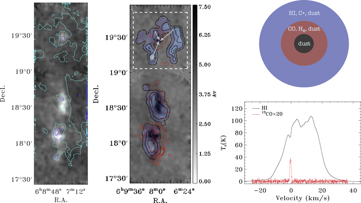
Figure 1. Temperature distribution, abundance distribution, onion-like model, and H iNSA feature. Left: the 2MASS extinction overlaid with the dust temperature. The contours from light blue to dark blue are 12 K, 13 K, and 14 K respectively. Middle: the 2MASS extinction overlaid with the ratio of [H i]/[H2] column densities (black contour and blue shadow), and [13CO]/[H2] column density (red) respectively. The black contours are at 10%, 40%, and 70% of maximum value of 2.1 × 10⁻². The red contours are at 10%, 30%, 50%, 70%, and 90% of maximum value. The maximum value is 2.1 × 10⁻⁶. The white arrows show the direction of the H i–H2 transition of B227. Right top: an onion-like model of evolving molecular cloud, which is a 2D version of the left image, corresponding to the source B227. Right bottom: H iNSA feature of the source B227 at velocity ≃−1 km s−1, with corresponding 13CO emission, which is from the center of B227.
Download figure:
Standard image High-resolution image3.1. Dust Temperature and Column Density
For each image pixel, an SED was extracted and fitted with a single-temperature modified blackbody of the form

where Ω is the solid angle of the emitting element, Bν is the blackbody emission from the dust at temperature Td, κν is the dust mass absorption coefficient, μ = 2.33 is the particle mass per hydrogen molecule, mH is the mass of hydrogen atom, and  is the column density of hydrogen molecules, and we assumed the gas-to-dust ratio is 100. In Equation (1),

is the Planck function and

(where κ230 = 0.009 cm2 g−1) is the emissivity of the dust grains at 230 GHz.
We used 2MASS extinction data to eliminate the column density of hydrogen atoms as a parameter for fitting the dust temperature Td and emissivity spectral index β. The hydrogen column density NH can be estimated from the optical extinction (Güver & Özel 2009),

As the atomic hydrogen fractional abundance is small, we take  and obtain

The column density of hydrogen molecules  is related to visual extinction Av,

Combined Herschel SPIRE 250, 350 and 500 μm data with 2MASS extinction data, the dust temperature Td, column density of hydrogen molecules  and emissivity spectral index β can be fitted simultaneously by using Equation (1).
3.2. Column Density of Cold Hi
The new Arecibo H i images provide us with the overall H iNSA distribution in these sources. In order to extract the absorption component, we subtracted a relatively uniform background by averaging the H i emission values from surrounding points of the clouds, which has been done in a fashion similar to that described by Knee & Brunt (2001). The method for solving for the optical depth of the absorbing gas is described from Equation (12) in Li & Goldsmith (2003),

where τ0 is the peak optical depth of the absorption feature at the centroid velocity,  is the foreground H i optical depth, taken to be 0.1, which is the typical value of the foreground H i and only results in 0.4% uncertainty of optical depth of H i. TH i is the quantity obtained from the spectrum by fitting a polynomial to the portion of the spectrum without the absorption, Tc is continuum temperature, taken to be 3.5 K, including the cosmic background and Galactic continuum emission. Tx is the excitation temperature of H i in the dark cloud, which could be replaced by the dust temperature, Tab is the absorption temperature, which is referred to as the depth of absorption line, p is the ratio of background H i optical depth τb to optical depth of the uniformed Galactic atomic gas τh (τb = pτh), τh is the total of the foreground H i optical depth and the background H i optical depth (τh = τf + τb), and p can be calculated from a model of the local H i distribution and is generally in the range of 0.8–0.9.
The column density of H i is given by

where ΔV is the FWHM of the absorption line from a Gaussian fit, and Tk is the kinetic temperature. We used the dust temperature Td derived from Herschel SPIRE maps as Tk, which should be well coupled in such clouds (Goldsmith & Li 2005). The column density of cold H i had been obtained based on H iNSA analysis.
Since the true total column density measurement will be affected by the optically thin approximation, several approaches have been employed to evaluate this potential problem. Lee et al. (2015) used two different methods to estimate the correction factor f for high optical depth and found that they are consistent, which is likely due to the relatively low optical depth and insignificant contribution from the diffuse radio continuum emission. As the clouds we study are located in the outer region of the Galaxy and the optical depths are small (Kolpak et al. 2002), the correction for the optical depth should not affect the H i column density significantly. The overall uncertainty is approximately 50%.
Since we cannot obtain the Tk, we present the upper and lower limit H i column density and H i abundance by using temperature of 10 and 30 K. The upper and lower limits for the H i column density for the three clouds are 7.50 × 1019 cm−2 and 2.31 × 1018 cm−2 respectively. The upper and lower limits for the H i abundance are 0.09 and 0.001 respectively.
3.3.
 Column Density

The central frequency of the 13CO J = 1–0 line ν is 110.2 GHz.
The column density of 13CO in the upper level (J = 1) can be expressed as

where k is Boltzmann's constant, h is Planck's constant, c is the speed of light, Aul is the spontaneous decay rate from the upper level to the lower level, and Tb is the brightness temperature. We obtain

The total 13CO column density Ntot is related to the upper level column density Nu through

where the level correction factor fu can be calculated analytically under the assumption of local thermal equilibrium (LTE) as

where gu is the statistical weight of the upper level. Tex is the excitation temperature and Q(Tex) = kTex/Be is the LTE partition function, where Be is the rotational constant (Tennyson 2005). The partition function can be expressed as Q(Tex) ≈ Tex/2.76 K. The correction factor for opacity fτ is defined as

and the correction for the background fb can be expressed as

where τ13 is the opacity of the 13CO transition and Tbg is the background temperature, which is assumed to be 2.7 K. The 13CO opacity is estimated under the assumption of being optically thin, for which fτ = 1. The excitation temperature Tex can be replaced by the dust temperature Td. The maximum 13CO column densities obtained using this analysis for the three sources B227, L1574, and CB45 are 4.1 × 1015 cm−2, 4.9 × 1015 cm−2, and 7.3 × 1015 cm−2. We then derived the 13CO abundance through column densities of dust and 13CO with consideration of other chemical effects, like 13CO depletion, and all of them are likely not dominant for our case.
Based on the dust data, the central volume densities of the three clouds, B227, L1574, and CB45 are 1600 cm−3, 2200 cm−3, and 1800 cm−3, assuming cloud sizes of 0.8 pc, 1.0 pc, and 1.5 pc respectively. The volume density is much greater than the 13CO critical density of 1266 cm−3, confirming the validation of the LTE assumption.
3.4. Abundances
The abundances of H iNSA and 13CO have been derived through a combined analysis with dust emission and extinction. We regarded the ratio between H i column density  and H2 column density
  as H i abundance ([H i]/[H2]). The 13CO abundance is derived from the ratio between 13CO column density
  and H2 column density
  ([13CO]/[H2]). We identified a striking "ring" of enhanced H i abundance, which is the first time such a structure has been seen in a molecular cloud. It closely resembles the "onion" shell description of a forming molecular cloud (Figure 1). The displacement between peak abundance positions of H i, 13CO, and dust indicates the ongoing H2 formation. Particularly, we find an orderly spatial variation of H i abundance between 2% and 0.2%. The distribution of H i abundance measured from H iNSA is also consistent with the inner cloud "core" being chemically more evolved, due to higher volume densities present there.
4. Model
4.1.
Formation Model

H2 formation occurs on the dust grain with a formation rate (Hollenbach & Salpeter 1971)

where  has units of cm−3 s−1,
  is the sticking efficiency,
  is the recombination efficiency, ngr (cm−3) is the atomic hydrogen density in the gas,
  is the mean velocity of atoms, σgr (cm2) is the cross section of grains, and ngr (cm−3) is the number density of grains.
The values and derivations of the parameters are taken from Goldsmith & Li (2005). The simplification of the H2 formation rate can be expressed as

We denote the H2 formation rate coefficient  as k' = 1.2−17 cm3 s−1 after taking the effect of grain size distribution into account (Goldsmith & Li 2005).
The formation rate coefficient k' is related to the grain size, namely the cross-section area of dust grains, which is connected to the thermal balance and the estimate of dust mass. Based on the study of grain size distribution from Mathis et al. (1977), the reasonable upper and lower limits of radii, amax = 10000 Å and amin = 25 Å, which enter as (amaxamin)−0.5, are adopted for evaluating the effect of the grain size distribution on the formation rate coefficient. In comparison with the standard grain radius 1700 Å, the formation rate coefficient is increased by a factor of 3.4. Combining the grain size distribution and other factors, the uncertainty of H2 formation rate coefficient may differ from its nominal value by a factor of 5. Although the nominal value of k' we take has large uncertainty, it is well beyond the goal of this paper to consider the overall context. Therefore, we are utilizing the most common value for the cross-section area of the dust.
The density of gas ngas can be regarded as total density n0 as n0 ∝ ngas. We derived the volume proton density of the clouds through the dust data. For the volume proton density, we derived the mean values from outer to inner of the cloud by assuming the cloud is spherical. It ranges from 102.9 cm−3 to 103.2 cm−3 approximately (Figure 2). The time dependence of the molecular hydrogen can be express as

where  is the cosmic-ray ionization rate. We defined the fractional abundance of atomic and molecular hydrogen,
  and
and  , as the density of species
  and
and  divided by the total proton density n0, then we find

Substituting  , we can rewrite this as

The time dependence of the fractional abundance of molecular hydrogen is then given by
The fractional abundance of atomic hydrogen is  and is given by
The timescale for H i to H2 conversion is given by

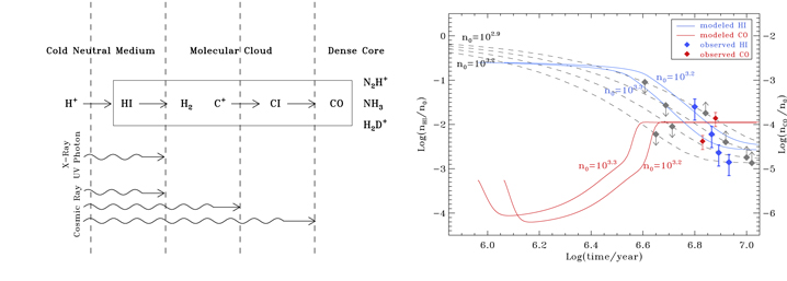
Figure 2. Chemical process and time-dependent model. Left: the chemical processes of diffuse CNM—molecular cloud—dense core. The processes in the square indicates the chemical evolution in our work, which is corresponding to the right plot. Right: time dependence of the fractional abundance of the atomic hydrogen and CO. The blue and red symbols represent the H i and CO observations, respectively. The four H i measurements are from the four points that are along the right top arrow of source B227 in Figure 1. The two CO measurements (from left to right) are the mean values from the outer envelop and inner core of the source B227, and the mean proton total densities are 102.9 cm−3 and 103.0 cm−3 respectively. The dashed lines represent the H2 formation model for clouds at different total proton densities n0. The blue and red lines represent the cloud evolution in a time-dependent chemical model with the abundance of H i and CO. The gray diamonds with upward and downward arrows represent the lower and upper limits of the H i abundances.
Download figure:
Standard image High-resolution image
We derived the timescales of these isolated dark clouds to be ∼6 Myr using H i abundance, total gas density, and gas temperature obtained according to the time dependence model described in this section (Figure 2). The upper and lower limits of H i abundances are plotted in Figure 2 and the points at upper limits represent the lower ages of the clouds for the fixed volume densities.
4.2. Chemical Model
We also use a two-stage young dark clouds formation collapse model. We assume that translucent clouds are the intermediate stage when diffuse clouds become young dark clouds. In the first stage, when diffuse clouds become translucent clouds, we only consider the H i → H2 transition process as discussed in the rest of the paper. In the second stage, we simulate a gas–grain reaction network to calculate the chemical evolution of species including H i and H2 in collapsing cores.
We use the Ohio State University gas–grain code. The gas–grain chemical reaction network is explained in Hincelin et al. (2011) and Hincelin et al. (2013). Moreover, the Kinetic Database for Astrochemistry (Wakelam et al. 2012) also has an electronic version of the network. We simulate the gas–grain chemistry in free-fall collapsing cores with initial hydrogen nucleus densities of 102.3 and 102.4 cm−3 and evolve to 103.2 and 103.3 cm−3 eventually. It takes 107 years to collapse to form a dense core. During free-fall collapse, the rate at which the density increase is give by Spitzer (1978). The collapsing process is isothermal with a constant temperature of 10 K, while the visual extinction varies from 1 to 4 mag. The cosmic-ray ionization rate is set to 5.2 × 10⁻¹⁷ s−1. The size of dust grains is assumed to be uniform, with a radius of 0.1 μm. The sticking coefficient is fixed to 1. The elemental abundances are assumed to be "low metal," as in Semenov et al. (2010). In our model, species in the young dark clouds are formed by the chemical evolution of species in translucent clouds. Thus, we use the observed abundances of species in translucent clouds in HD 24534, HD 154368, and HD 210121 (Sofia et al. 2004; Sonnentrucker et al. 2007; Weselak et al. 2009; Burgh et al. 2010), where the atomic H density is about a quarter of the total H nucleus density of the initial abundances in our calculation of the second stage. If a species is observed in more than one source, we take the average of the observed values in different sources. Table 1 shows the initial abundances used in our calculation. Through this time-dependent chemical model, we compared the timescales of cloud evolution traced by the abundance of H i and CO with our observed abundances and calculated timescale. The observed H i abundance and timescale of cloud formation is partially consistent with the chemical model. On the other hand, CO abundance is only marginally consistent with the chemical model, which already evolved into the steady state at the corresponding abundance (Figure 2).
Table 1. Initial Abundances Used in the Chemical Model
| Element | Abundance |
|---|---|
| C | 4.34 × 10⁻⁷ |
| H | 2.50 × 10⁻¹ |
| He | 9.00 × 10⁻² |
| N | 7.60 × 10⁻⁵ |
| O | 2.50 × 10⁻⁴ |
| C2 | 1.79 × 10⁻⁸ |
| CH | 1.59 × 10⁻⁸ |
| CN | 6.79 × 10⁻⁹ |
| CO | 5.45 × 10⁻⁶ |
| H2 | 3.75 × 10⁻¹ |
| NH | 1.78 × 10⁻⁹ |
| OH | 4.36 × 10⁻⁸ |
| C+ | 1.14 × 10⁻⁴ |
| Cl+ | 1.00 × 10⁻⁹ |
| Fe+ | 3.00 × 10⁻⁹ |
| Mg+ | 7.00 × 10⁻⁹ |
| Na+ | 2,00 × 10⁻⁹ |
| P+ | 2.00 × 10⁻¹⁰ |
| S+ | 8.00 × 10⁻⁸ |
| Si+ | 8.00 × 10⁻⁹ |
| CH+ | 5.51 × 10⁻⁹ |
| e | 1.14 × 10⁻⁴ |
Download table as: ASCIITypeset image
5. Discussion
It has been rare to have both H i and H2 measured for the same regions in the Galaxy. Lee et al. (2015) used the integrated H i emission flux in channels, the range of which was determined by correlation with 2MASS extinction. Such a priori requirements of H i mimicking dust diminish the logical credence of H i emission tracing the atomic component within a molecular cloud. Fukui et al. (2014) found an optically thick H i emission envelope around a molecular cloud. In this work, utilizing H iNSA, we discovered a chemically young molecular cloud undergoing H2 formation, revealed by a prominent "ring" of self-absorption tracing atomic hydrogen mixed with molecules. We derived the formation timescale to be ∼6 Myr, consistent with both an analytical model and a numerical chemistry model. Our results could further test recent H2 formation models in different contexts (Sternberg et al. 2014; Bialy et al. 2017).
Our results can also help constrain galaxy evolution simulations. A key recent development is the implementation of the physics of molecular hydrogen and star formation prescription based on the local molecular hydrogen density rather than the total hydrogen density (Zemp et al. 2012). In Gnedin & Kravtsov (2011), only two types of observations were able to calibrate the H2 formation rate in different environments, UV absorption in diffuse regions and H iNSA in dense clouds. This work further improves the accuracy of the H iNSA measured H2 formation rate.
Both the timescale and H i abundance distribution of the clouds are inconsistent with fast H2 formation (Glover & Mac Low 2007), which relies on stochastic processes of localized high volume H i density. Such a fast cloud formation model could produce a significant amount of molecular hydrogen, e.g., for cooling in a short time, but cannot convert the vast majority of the gas into molecular form, which is our key finding here. The fact that more than 99% of the protons have been turned into H2 requires millions of years and comprehensive global H2 formation, not just in pockets of locally enhanced condensations. The observed Mach number of the clouds is more than 20, which elevates the inconsistency between our observation and the fast cloud formation model.
The total column densities found in these isolated dark clouds are consistent with commonly used initial conditions for protoplanetary disks. However, the measured H i abundance is one to a few orders of magnitude higher than those assumed in such models (e.g., Walsh et al. 2015). In these models, the H i abundance keeps dropping with time and impacts subsequent chemical reactions. We expect our measured value to affect future consideration of chemical evolution of disks. All the above statements indicate that the parameters of galactic H2 formation play a crucial role in both galaxy evolution and star formation.
6. Summary
We mapped H i, 13CO J = 1–0 emission, and dust continuum emission of isolated dark clouds, B227, CB45, and L1574. The combined analysis of H iNSA, CO emission, dust emission, and extinction enables us to directly measure the variation H i abundance in these transition clouds. The timescale of the clouds had been examined through an analytical model. Our main results are the following.
- 1.We identified a striking "ring" of enhanced H i abundance, which is the first time such a structure has been seen in a molecular cloud. It closely resembles the "onion" shell description of a forming molecular cloud (Figure 1). The displacement between peak abundance positions of H i, CO, and dust indicates the ongoing H2 formation. Particularly, we find an orderly spatial variation of H i abundance between 2% and 0.2%.
- 2.We derived the H i–H2 evolutionary timescales for these isolated dark clouds to be ∼6 Myr and further examined the cloud evolution through a time-dependent chemical model.
- 3.Our results could test H2 formation models, constrain galaxy evolution simulations, and may affect future consideration of chemical evolution of disks, all of which indicate that the parameters of galactic H2 formation play a crucial role for both galaxy evolution and star formation.
This work is supported by National Key R&D Program of China grant No. 2017YFA0402600, the National Natural Science Foundation of China grant No. 11725313 and No. 11690024, and the International Partnership Program of Chinese Academy of Sciences grant No. 114A11KYSB20160008. The Arecibo Observatory is operated by SRI International under a cooperative agreement with the National Science Foundation (AST-1100968), and in alliance with Ana G. Méndez-Universidad Metropolitana, and the Universities Space Research Association. D.L. acknowledges support from "CAS Interdisciplinary Innovation Team" program. This work was carried out in part by the Jet Propulsion Laboratory, which is operated by NASA through the California Institute of Technology. Z.Y.Z. acknowledges support from ERC in the form of the Advanced Investigator Programme, 321302, COSMICISM.
Footnotes
- 11
http://herschel.esac.esa.int/hipe/; version 13.0.0.