


Abstract
Using the times of light maximum collected from the GEOS RR Lyrae database and determined from sky surveys, we utilize the O − C method to study the period variations of seven field ab-type RR Lyrae stars. The time coverage of data for most stars is more than 100 years, allowing us to investigate period changes over a large time span. We find that the O − C diagrams for most stars can be described by a combination of cyclic variations and long-term period changes. Assuming the former were caused by the light-travel-time effect, the pulsation and orbital parameters are obtained by the nonlinear fitting. We find that the orbital periods in our sample range from 33 to 78 years, and the eccentricities are relatively higher than the results for other candidates (e > 0.6). The minimal masses of the potential companions of XX And, BK Dra, and RY Psc are less than one solar mass, and those of SV Eri, AR Her, and RU Scl are 3.3, 2.1, and 3.4 M⊙, respectively. Moreover, we suggest that the companion of AR Her may be a blue straggler that experienced mass transfer or a merger of two stars. The O − C diagram for ST Vir also shows distinct long-term period decrease, and in the O − C residuals, additional quasi-periodic variations that can be described by damped oscillation are found. Combining the data from the literature and our analysis, we plot the log P–AO−C diagram. The distribution of our binary candidates suggests that their period variations are not caused by the Blazhko effect.
1. Introduction
RR Lyrae stars are a type of short-period, pulsating variable star, and are widespread in the universe. They are old, low-mass stars in the core-helium stage of evolution (Salaris & Cassisi 2005). In the Hertzsprung–Russell diagram, they are located on the intersectional region of the classical Cepheid instability strip and the horizontal branch. Since being discovered, they have been studied for more than 100 years. Because of the period–luminosity relation in the infrared, such stars are often used as standard candles to detect the distance of the Milky Way and nearby galaxies (Karczmarek et al. 2017; Iorio et al. 2018), used as tracers to investigate the chemical and dynamical properties of old stellar populations (Skowron et al. 2016), and used to test the theories of the evolution of low-mass stars and stellar pulsations (Iben & Rood 1970; Bono & Stellingwerf 1994).
For pulsating variable stars, the pulsation parameter that can be determined easily and directly is the pulsation period , which is related to the structure of the star by the pulsation equation , where and are the values of the mean density of the star and Sun, respectively, and Q is the pulsation constant (Preston 1961). From this, we can see that the stellar evolution would influence the pulsation period through the change of the mean density. Actually, the monotonic decades-long period changes were used to study the stellar evolution (Le Borgne et al. 2007), and the short-term period changes were used to analyze the famous phenomenon in RR Lyrae stars, the Blazhko effect (Blažko 1907), which manifests as periodic modulations of the light curves on timescales typically of tens of days to hundreds of days (Jurcsik et al. 2005; Benkő et al. 2014; Skarka 2014; Skarka et al. 2016b). The principle tool to analyze the period changes of variable stars is the O − C diagram, which stands for Observed minus Calculated (Sterken 2005). For RR Lyrae stars, usually the observed times of light maximum are used as O, and C can be obtained from adopted linear ephemeris. The O − C diagrams showing parabolic curves caused by secular period shortening/lengthening, are usually attributed to the evolutionary period changes (Lee 1991), and the Blazhko effect makes the O − C curves show cyclic variations via the Blazhko periods. Moreover, the O − C diagrams of some RR Lyrae stars are more complicated. Le Borgne et al. (2007) presented some examples of O − C patterns that show irregular variations or abrupt changes, and concluded that the corresponding physical explanations should be searched for within the stellar structure.


However, the pulsation periods also can be influenced by a dynamic effect, like the light-travel-time effect (LiTE), which is caused by the star orbiting in a binary system (Irwin 1952). If the motions exist, the O − C patterns show periodic oscillations. Recently, Li & Qian (2014) used the Kepler data to analyze the 21 non-Blazhko RRab stars, and found that 2 stars, FN Lyr and V894 Cyg, had low-mass companions on wider orbits. Hajdu et al. (2015) searched for binary RR Lyrae stars in the OGLE-III and IV Galactic bulge data, and provided a sample of 12 firm binary candidates from the analysis of 1952 well observed RR Lyrae stars. They estimated that ≥4% of the RR Lyrae stars reside in binary systems. Liška et al. (2016a, 2016b) used the times of maxima adopted from the GEOS database5 (Le Borgne et al. 2007) together with those determined from sky surveys and their new measurements for O − C analysis. They restudied the binarity of TU UMa, detected new binary candidates of RR Lyrae stars, and provided the corresponding discussions. In these works, the O − C method plays an important role in determining the companions of pulsating stars and in deriving the orbital elements (Paparo et al. 1988).
Binary and multiple systems are common in the universe (e.g., Duchêne & Kraus 2013), and many types of variable stars have been found to exist in binary and multiple systems (Zhou 2010), but RR Lyrae stars were rarely found in binary systems (see the overview in Section 2 in Liška et al. 2016b). Until now, several tens of thousands of RR Lyrae stars were known (Watson et al. 2006; Soszyński et al. 2014, 2016), but only less than one hundred RR Lyrae binary candidates were identified(Liska & Skarka 2016). This is in clear contrast with what we observe in other types of stars. The reasons for this phenomenon may be related to the evolutionary history of RR Lyrae stars. Some authors have pointed out that RR Lyrae binaries are expected to have long orbital periods and wide orbital distances, and would be hardly detectable (Li & Qian 2014; Skarka et al. 2016a). However, it is worthwhile to invest time and effort into searching for RR Lyrae stars in binary systems. For example, if an RR Lyrae star was found in an eclipsing system (Pietrzyński et al. 2012), its mass could be determined independently, and could be used to check the values from pulsation and evolutionary models (e.g., Lee & Demarque 1990). These detecting works can improve our understanding of the evolution processes and environments of RR Lyrae stars and other horizontal branch stars, and provide useful references for evolution theory.
This work is inspired by Liška et al. (2016b), and the GEOS maxima database is used as the main source of data. Besides the stars discussed in Liška et al. (2016b), we also find that the O − C diagrams of seven additional RRab stars show cyclic variations. The variations of several stars have been noted in previous literature (Firmanyuk 1982; Le Borgne et al. 2007), but there is no further study. In order to investigate these stars, we collected the published times of light maximum from GEOS, determined new times of light maximum from various sky surveys, and studied the O − C patterns by nonlinear fitting. Sections 2 and 3 describe the data collection and the O − C analysis. A discussion and a summary are presented in Sections 4 and 5, respectively.
2. Data Collection
The GEOS maxima database provides tens of thousands of times of light maximum to thousands of RR Lyrae stars collected from the literature and obtained from the automated observations with TAROT (Bringer et al. 1999; Klotz et al. 2008). In this paper, we focus on the RRab stars, and the selection is based on Le Borgne et al. (2007), in which 123 RRab stars with clear O − C diagrams have been analyzed to study the stellar evolution. We utilize the times of light maximum provided by GEOS for the pre-analysis, and find that besides the stars discussed in Liška et al. (2016b), the O − C diagrams of seven RRab stars (XX And, BK Dra, SV Eri, AR Her, RY Psc, RU Scl, and ST Vir) also show cyclic variations. Table 1 lists some basic information for these stars, including the star names, coordinates, magnitudes, linear ephemeris, metallicities, and masses. Table 2 lists the times of light maximum provided by the GEOS database, but the data marked as "pr. com." are not included.
Table 1. Information on the Seven RRab Stars
| Star Name | R.A. (h:m:s) | Decl. (°:':'') | Mag range (V) | T0 (HJD) | (days) | [Fe/H] | M1 (M⊙) | Time Coverage (years) |
|---|---|---|---|---|---|---|---|---|
| XX And | 01:17:27.4 | +38:57:02 | 10.08–11.13 | 2439087.436 | 0.722753189 | −2.01 (1) | 0.63 | 114(1902–2016) |
| BK Dra | 19:18:20.7 | +66:24:48 | 10.59–11.87 | 2425523.305 | 0.5920792 | −2.12 (1) | 0.64 | 118(1897–2015) |
| SV Eri | 03:11:52.1 | −11:21:14 | 9.56–10.23 | 2435552.109 | 0.7137709 | −2.04 (1) | 0.63 | 112(1904–2016) |
| AR Her | 16:00:32.2 | +46:55:26 | 10.59–11.63 | 2438882.915 | 0.470007955 | −1.30 (2) | 0.57 | 120(1896–2016) |
| RY Psc | 00:11:41.1 | −01:44:55 | 11.82–12.72 | 2442681.147 | 0.52973131 | −1.39 (1) | 0.57 | 102(1912–2014) |
| RU Scl | 00:02:48.1 | −24:56:43 | 9.543–10.749 | 2431122.839 | 0.49333478 | −1.25 (1) | 0.56 | 85(1927–2012) |
| ST Vir | 14:27:39.1 | −00:54:06 | 10.838–12.154 | 2440736.374 | 0.410824 | −0.88 (1) | 0.53 | 120(1894–2014) |

Notes. The magnitude ranges are taken from VSX (Watson et al. 2006). The masses of stars are calculated by Equation (22) in Jurcsik (1998). The time coverage means the span of the times of light maximum.
References. (1) Layden (1994); (2) Feast et al. (2008).
Download table as: ASCIITypeset image
Table 2. The Times of Light Maximum of the Seven RRab Stars Obtained from the GEOS Database
| HJD_Max | Error | Method | References |
|---|---|---|---|
| (days) | |||
| XX And | |||
| 2415760.6810 | 0.01 | pg | Ashbrook J., 1949, AJ 54, 176 |
| 2418024.9450 | ⋯ | pg | Ashbrook J., 1949, AJ 54, 176 |
| 2421031.7020 | 0.01 | pg | Ashbrook J., 1949, AJ 54, 176 |
| 2424134.4640 | 0.01 | ⋯ | Azarnova T.A., 1963a, VS 14, 485 |
| 2424171.3300 | 0.01 | ⋯ | Azarnova T.A., 1963a, VS 14, 485 |
| 2424184.3520 | 0.01 | ⋯ | Azarnova T.A., 1963a, VS 14, 485 |
| 2424192.2700 | 0.01 | ⋯ | Azarnova T.A., 1963a, VS 14, 485 |
| 2424204.5690 | 0.01 | vis | Lange G.A., 1957, AC 176, 14 |
| 2424317.3160 | 0.01 | vis | Tsesevich V.P., 1947b, Odessa Izv. 1, 1 |
| 2424353.4220 | 0.01 | ⋯ | Azarnova T.A., 1963a, VS 14, 485 |
| ⋯ | ⋯ | ⋯ | ⋯ |
Note. The column abbreviations are defined as follows: vis—visual; pg—photographic; pe—photoelectric; CCD—charge coupled device; dslr—digital single lens reflex camera. More detailed information also can be obtained by accessing the website (http://rr-lyr.irap.omp.eu/dbrr/). The date when the data were acquired from GEOS is 2017 November 8.
Only a portion of this table is shown here to demonstrate its form and content. A machine-readable version of the full table is available.
Download table as: DataTypeset image
These stars were observed by several sky surveys, including DASCH (Grindlay et al. 2009), NSVS (Woźniak et al. 2004), ASAS (Pojmanski 1997), OMC (Mas-Hesse et al. 2003; Zejda & Domingo 2011), CRTS (Drake et al. 2009), SWASP (Pollacco et al. 2006; Butters et al. 2010), and QES (Bramich et al. 2014). Using the light curve data from these surveys, we determine many new times of light maximum for our study. Table 3 lists the numbers of new data from various surveys. Note that the common method to determine the times of light maximum is to fit algebraic polynomials around the extremum (Sterken 2005), and only the data points near the extremum are used in the fitting. This method is suitable for analyzing these data from SWASP and QES, but not for those data with lower time resolutions (DASCH, NSVS, ASAS, OMC and CRTS). Therefore, we use a determining method similar to that of Li & Qian (2014) and Li et al. (2018b) to analyze the data from these latter surveys. Using DASCH data as an example, we first divide the data into different groups; fit third-order Fourier polynomial to the data; and determine the times of light maximum using the calculated first derivatives (see Figure 1). In the fitting, all the data points are used to determine the times of light maximum. Depending on the different time resolutions, the orders of the Fourier polynomials are 3 (DASCH and CRTS) or 5 (ASAS, NSVS, and OMC). Table 4 lists these new times of light maximum from the sky surveys. Figure 2 shows the O − C diagrams for these RRab stars, from which the variations can be clearly seen.

Figure 1. Phased light curves of BK Dra from DASCH as an example. About 150 points between HJD 2418428 and 2421796 are used in the detection. The solid line, which also has been phased, is the third-order Fourier polynomial fit to the data. The full black circles indicate the positions of light maximum.
Download figure:
Standard image High-resolution image
Figure 2. O − C diagrams of the seven RRab stars. The open circles and triangles indicate that the data are obtained from the GEOS database and sky surveys, respectively. The unused data are marked with crosses.
Download figure:
Standard image High-resolution imageTable 3. Numbers of New Times of Light Maximum Determined from the Sky Surveys
| Star Name | Numbers |
|---|---|
| XX And | NSVS(1), SWASP(22) |
| BK Dra | DASCH(37), NSVS(1), OMC(1), QES(30) |
| SV Eri | ASAS(5) |
| AR Her | DASCH(35), NSVS(1), CRTS(1) |
| RY Psc | NSVS(1), ASAS(4), CRTS(2), QES(20) |
| RU Scl | NSVS(1), ASAS(4), CRTS(1), SWASP(30) |
| ST Vir | DASCH(38), NSVS(2), ASAS(6), CRTS(7), |
| QES(46), OMC(1) |
Download table as: ASCIITypeset image
Table 4. Times of Light Maximum of the Seven RRab Stars Determined from the Sky Surveys
| HJD_Max | Error | References |
|---|---|---|
| 2400000+ | (days) | |
| XX And | ||
| 51417.7094 | 0.0012 | NSVS |
| 54324.6217 | 0.0005 | SWASP |
| 54329.6801 | 0.0005 | SWASP |
| 54332.5708 | 0.0006 | SWASP |
| ⋯ | ⋯ | ⋯ |
Only a portion of this table is shown here to demonstrate its form and content. A machine-readable version of the full table is available.
Download table as: DataTypeset image
3. O − C Analyses and Results
Assuming that the periodic variations in O − C diagrams were caused by LiTE, the nonlinear fittings are applied on these RRab stars, and the fitting formulae are

and
where ΔT0 and ΔP0 are the correction values of the initial epoch and pulsation period, and β is the linear change of the pulsation period (day cycle−1). A, e, ω, Porb, and T are the orbital parameters (Porb and T are not explicitly contained in Equation (2), but relate to E*; see Table 5 or Li & Qian 2010, 2014 for details). In the fitting, all the variations are modeled simultaneously. The errors of these parameters, covering the 68% confidence interval, are the unbiased standard errors. The weights of the O − C data points are dependent on the observed methods: those obtained visually or photographically (vis or pg) are set as 1, and those obtained with electronic devices (pe or CCD) are set as 10. A few data points with large deviations (see the data points marked as crosses in Figure 2) are not used in analysis. Our results show that the O − C patterns of most stars can be interpreted as long-term period changes plus cyclic changes; one star (ST Vir) can be described by a long-term period decrease and quasi-periodic variation. The details of our studies are provided in the following subsections.
Table 5. Pulsation and Orbital Parameters of the Six RRab Stars
| Star | [cor] | T0 [cor] | β | A | e | ω | T | f(m) | K1 | |||
|---|---|---|---|---|---|---|---|---|---|---|---|---|
| (days) | 2400000+ | (day Myr−1) | (days) | (au) | (°) | (years) | 2400000+ | (M⊙) | (km s−1) | (10−5 days) | ||
| XX And | 0.72275396(6) | 39087.4542(17) | 0.100(7) | 0.027(2) | 4.70(.27) | 0.68(7) | 268(7) | 60.9(1.8) | 40804(672) | 0.028(5) | 3.1(4) | 1.52(17) |
| BK Draa | 0.59207896(22) | 25523.3553(31) | −0.025(6) | 0.064(8) | 11.2(1.4) | 0.77(6) | 161(4) | 75.3(1.1) | 43453(296) | 0.25(9) | 7.0(1.2) | 2.8(.5) |
| BK Drab | 0.59207802(4) | 25523.3575(30) | ⋯ | 0.059(5) | 10.2(0.9) | 0.70(6) | 157(5) | 78.4(.8) | 43717(378) | 0.17(4) | 5.4(.7) | 2.1(.3) |
| SV Eri | 0.71377169(60) | 35552.2194(105) | 1.885(25) | 0.079(6) | 13.7(1.0) | 0.78(11) | 94(13) | 33.1(.5) | 29207(374) | 2.3(.5) | 19.8(3.7) | 9.4(2.2) |
| AR Her | 0.47000806(7) | 38883.0540(46) | −0.396(8) | 0.066(6) | 11.4(1.1) | 0.64(9) | 43(6) | 34.2(.3) | 21113(207) | 1.3(.4) | 12.9(1.8) | 4.1(.6) |
| RY Psc | 0.52973142(15) | 42681.1249(47) | 0.182(10) | 0.061(22) | 10.6(4.9) | 0.9(fixed) | 341(9) | 65.8(.9) | 27707(320) | 0.28(.30) | 11.0(6.4) | 3.9(2.2) |
| RU Scl | 0.49333005(37) | 31122.8605(44) | 0.543(10) | 0.086(24) | 14.8(4.2) | 0.84(10) | 324(12) | 35.7(.4) | 30554(380) | 2.56(2.16) | 22.7(9.1) | 7.5(3.0) |


Notes. The column abbreviations are defined as follows: star—star name; [cor]—corrected pulsation period; T0 [cor]—corrected epoch; β—linear changes of pulsation period in day Myr−1; A— in light days, where a1 is the semimajor axis, i is the inclination angle, and c is the speed of light; e—the eccentricity; ω—longitude of the periastron passage in the plane of the orbit; Porb—orbital period of the binary system; T—time of passage through the periastron; f(m)—mass function of companion; K—velocity semi-amplitude in km s−1; —range of the pulsation period in days.
amodel 1 = parabola + LiTE. bmodel 2 = linear revise + LiTE.


Download table as: ASCIITypeset image
3.1. XX And
The quasi-periodic variation in the period of XX And has been found by Firmanyuk (1982). In that paper, the O − C diagram of XX And is plotted by only a dozen points. Based on the longer baseline of O − C data, Le Borgne et al. (2007) pointed out that this star showed a linearly increasing period with a rate of 0.144 ± 0.007 day Myr−1. Our result shows that besides the increasing period, the O − C diagram also displays cyclic variation that can be explained by LiTE. Figure 3 shows the corresponding O − C diagram, in which the linear ephemeris in Table 1 is used. The solid line in the top panel refers to the combination of parabolic variation and the cyclic change, and the dashed line represents the parabolic variation that reveals a linear change of the pulsation period; the solid line in the middle panel refers to the cyclic change O − C1, where the long-term period change has been subtracted; the residuals after cyclic change removal are shown in the bottom panel. The pulsation and orbit parameters are listed in Table 5.

Figure 3. O − C diagram of XX And. In the top panel, the linear ephemeris in Table 1 is used to calculate the O − C values. The solid line in the top panel refers to the combination of parabolic variation and the cyclic change, and the dashed line represents the parabolic variation that reveals the linear change of the pulsation period; the solid line in the middle panel refers to the cyclic change O − C1, where the long-term period change has been subtracted; the residuals are shown in the bottom panel.
Download figure:
Standard image High-resolution imageThe long-term period change rates β of XX And, 0.100 ± 0.007 day Myr−1, is different from previous literature, but combining with the cyclic change, they can describe the O − C diagrams well. If the cyclic changes were caused by LiTE, using the mass function, we can obtain the minimal masses of components. Assuming the mass of XX And is 0.63 M⊙ (see Table 1), our calculations give the result that the minimal companion mass of XX And is 0.3 M⊙.
3.2. BK Dra
Due to the differences in systemic radial velocities up to several tens of km s−1, BK Dra was identified as a candidate for spectroscopic binary (Fernley & Barnes 1997). Le Borgne et al. (2007) pointed out that the O − C diagrams of five RRab stars (EZ Lyr, RV UMa, BK Dra, SS Tau, and BN Vul) shown small amplitudes, resulting in more scattered plots. Actually, the variations in some of those stars can be explained as the LiTE of a companion in an elliptical orbit. Liška et al. (2016b) proposed that one of the stars, RV UMa, is an RR Lyrae binary candidate. Its O − C pattern can be considered LiTE, as it has a period of 66.9 years supplemented by a long-term period increase with a rate of 0.0172 day Myr−1. We also focused on these stars, and found that the O − C diagrams of two stars, EZ Lyr and BK Dra, show cyclic changes. However, even though the fitting curve can describe the O − C diagram well, the errors of the fitting results in EZ Lyr are much larger, indicating the result is unauthentic. Therefore, EZ Lyr is not in the scope of this paper.
We find that the O − C diagram of BK Dra can be described by two different models (model 1: parabola + LiTE; model 2: linear revise + LiTE). In model 2, the fitting parameter β is ignored. Figure 4 shows the O − C diagrams, and Table 5 lists the corresponding results. Using an F-test, we find that model 1 does not show any obvious improvement over model 2. This means that the long-term period change is not significant, and model 2 can describe the variations well enough. Model 2 for BK Dra gives an orbital period of 78.4 years and a minimal companion mass of 0.7 M⊙ (assuming the mass of BK Dra is 0.64 M⊙; see Table 1).
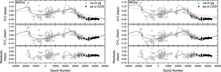
Figure 4. O − C diagrams of BK Dra with model 1 (left sub-figure) and model 2 (right sub-figure). It can be seen that in the left sub-figure the long-term period change is not significant. The data points and lines have the same definitions as those in Figure 3.
Download figure:
Standard image High-resolution imageIn the residuals of BK Dra, the early data points show more scatter than the new data (see the empty circles in the bottom panel of Figure 4). Note that these points are determined from pg data, which should have the same source as data provided by DASCH. We are not sure of the details of their determining methods. Those old times of light maximum were probably determined by one or several bright measurements, which were not necessarily very close to maximum, and these methods would give a very high dispersion to O − C diagrams. It can be seen in Figure 2 that the pg O − C points of BK Dra determined by us are relatively centralized, which demonstrate the suitability of our determining method.
3.3. SV Eri
The change in the O − C diagram of SV Eri was noted by Firmanyuk (1976, 1982). However, the cyclic change with large amplitude shown in Firmanyuk (1982) should have been caused by the cycle-count errors that occurred in the first two data points (Sterken 2005). Based on the data spanning a longer timescale, Le Borgne et al. (2007) found that SV Eri shows a linearly increasing period with the largest rate, 2.121 ± 0.031 day Myr−1, which is one order of magnitude larger than the average value (0.14 day Myr−1). They also noted the relative long period of SV Eri (0.71 day), and supposed that it seemed to have entered the rapid final phase of horizontal branch evolution.
We note that except for the upward parabolic component in the O − C diagram, SV Eri shows an additional cyclic change with small amplitude. Our LiTE fitting finds the O − C diagram of SV Eri can be described by the combination of a long-term period change with a rate of 1.885 ± 0.025 day Myr−1 and a periodic variation with a period of 33.1 ± 0.5 years. Figure 5 shows the corresponding O − C diagrams. It can be seen that the cyclic change in the O − C1 diagram is more obvious in the pe and CCD data. Assuming the mass of SV Eri was 0.63 M⊙ (see Table 1), the minimal mass of the potential companion should be about 3.3 M⊙, which means that it might be a black hole.

Figure 5. O − C diagrams of SV Eri. The data points and lines have the same definitions as those in Figure 3.
Download figure:
Standard image High-resolution image3.4. AR Her
Preston (1959) found that the hydrogen line of AR Her at minimum light is systematically stronger than those of other RRab stars. Moreover, Sturch (1966) obtained photoelectric observations on the UBV system of more than one hundred RRab stars, and found that the color index of AR Her at minimum light, B − V = 0.353, is smaller than that of other RRab stars, indicating that AR Her shows bluer color and higher temperature. Kinman & Carretta (1992) presented a study of another RRab star, BB Vir, which also shows a relatively small color index at minimum light (B − V = 0.23, Bookmeyer et al. 1977), and they found that the presence of a horizontal branch companion on the blue side of the instability strip can explain the abnormal color and the low amplitude in the light curves of BB Vir. Considering a similar situation, they pointed out that AR Her might be a binary composed of an RRab star with a period of 0.47 day and a c-type RR Lyrae star with a period of 0.233 day, where the latter provides more blue color to the system. However, the binary model was doubted by Smith et al. (1999). They pointed out that the light curve modulation of AR Her could not be produced by the superposition of the light curves of an RRab and an RRc star, but can be interpreted as complex Blazhko modulation. Moreover, they also pointed out that the coincident changes in the primary and Blazhko period may possibly occur in AR Her.
The O − C diagram of AR Her in Firmanyuk (1982) showed a cyclic change with high amplitude. Based on the data spanning a longer timescale, Le Borgne et al. (2007) pointed out that AR Her shows irregular variation. However, we find that the O − C diagram of AR Her can be described by a linearly decreasing period (−0.396 ± 0.008 day Myr−1) and a cyclic variation. Figure 6 shows the corresponding O − C diagram, and Table 5 lists the pulsation and orbit parameters. Our result gives an orbital period of 34.2 ± 0.3 years and minimal mass of the companion of 2.1 M⊙ (assuming the mass of AR Her is 0.57 M⊙; see Table 1).

Figure 6. O − C diagram of AR Her. The data points and lines have the same definitions as those in Figure 3.
Download figure:
Standard image High-resolution imageNoting the anomalous color index of AR Her at minimum light, there is a possibility that the companion is a blue straggler (BS) in the main-sequence stage. Assuming that the pulsating component of AR Her has the normal properties of an RRab star (at minimum light phase, B − V ≃ 0.42, Kinman & Carretta 1992, and absolute magnitude MV(min) ≃ 1.3 mag), and the companion is an A6 main-sequence star (B − V = 0.17, MV = 2.1, Adelman 2004), then the combined color index can be calculated and the result is B − V ∼ 0.333, which coincides with the value determined by Sturch (1966; see Table 1 in that paper). However, in a binary system, the more massive companion should be more evolved than the less massive one, unless the former is a BS that experienced mass transfer or a merger of two stars. See Section 4.2 for a more detailed discussion.
AR Her exhibits strong Blazhko modulation (especially the amplitude variation in light curves) with a period of about 32 days (Wischnewski 2016 and references therein). We use the software Period04 (Lenz & Breger 2005) to search for variations caused by the Blazhko effect in the O − C residuals. In the analysis, only recent photoelectric and CCD data are used. We find a significant peak in the frequency spectrum (see the upper panel of Figure 7). The corresponding value is fbl = 0.014694(1) cycle−1 = 0.031263(3) day−1, and the period is Pbl = 31.987(3) days, which is in agreement with previous results. It can be seen in the spectrum that there are side peaks around the fbl, and the frequency differences are about 0.00127 cycle−1, or 0.00270 day−1, which corresponds to a year (365.25 days or 0.00274 day−1). The bottom panel of Figure 7 shows the phased O − C residuals. Noting that the curve is asymmetric, we find that second-order Fourier polynomial can fit the curve well. The solid line in the bottom panel of Figure 7 refers to the corresponding fitting, and the amplitudes of the Blazhko component (fbl) and its harmonics (2fbl) are 0.0207(8) and 0.0072(8) days, respectively.

Figure 7. Upper panel: Fourier spectra of the O − C residuals (see the bottom panel of Figure 6) for AR Her. Bottom panel: O − C residuals of AR Her phased with the Blazhko period of 31.987 days. The solid line refers to the second-order Fourier polynomial fitting to the data.
Download figure:
Standard image High-resolution imageIn the O − C residuals around epoch number 0 (see the bottom panel of Figure 6), AR Her shows irregular variation, which deviate from our predicted trend of change. It seems that the variation is not repeated, but is an abrupt change. The cause of this phenomenon may be related to accidental internal changes of AR Her. As a star that has complex period variations, AR Her is worthy of continuous monitoring to achieve more information on the period changes.
3.5. RY Psc
Firmanyuk (1982) also noticed the cyclic change in the O − C diagram of RY Psc, but based on the data spanning a longer timescale, the parabolic component is more obvious than the periodic variation (Le Borgne et al. 2007). Therefore, we fit the data by using model 1, and find that the O − C diagram can be interpreted as a long-term period change with a rate of 0.182 ± 0.010 day Myr−1 and a periodic variation with a period of 65.8 ± 0.9 years. Note that, in the analysis, the parameter eccentricity is close to 1, so we fix it as 0.9 in our fit (see Table 5). Figure 8 shows the corresponding O − C diagrams. Assuming the mass of RY Psc was 0.57 M⊙ (see Table 1), the minimal mass of the potential companion should be about 0.8 M⊙, which means that it might be a compact star (e.g., white dwarf).

Figure 8. O − C diagrams of RY Psc. The data points and lines have the same same definitions as those in Figure 3.
Download figure:
Standard image High-resolution imageRY Psc was found to exhibit the Blazhko effect with a period of about 154 days using ASAS data (Szczygieł & Fabrycky 2007; Skarka 2014). We tried to search for the periodicity in the O − C residuals, but found that the frequency spectrum does not show any peak in the corresponding position. This result should be due to the smaller amount of O − C data. The light curves of PY Psc observed by QES (Bramich et al. 2014) clearly show amplitude modulation (AM; see Figure 9). The bottom panel of Figure 9 shows the folded light curves phased with mean pulsation period, where the amplitude variations can be seen clearly. However, the QES data only span about 83 days, which is shorter than the predicted Blazhko period. Maybe more monitoring on this star is needed to check for the Blazhko period.

Figure 9. Upper panel: the light curves of RY Psc observed by QES. Bottom panel: phased light curves of RY psc, which show clear amplitude modulation.
Download figure:
Standard image High-resolution image3.6. RU Scl
In the O − C diagram of RU Scl, there is a large gap between epoch number 20,000 and 35,000, which may introduce the cycle-count error. In situation I (see Figure 10), the O − C curves can be described by a long-term period increase with a rate of 0.327 ± 0.015 day Myr−1 and a cyclic change with a period of 48.6 ± 0.9 years. However, if we move the O − C points above a pulsation period of 35,000 (situation II), the O − C curves can be fit by a parabola. In order to confirm which situation is true, we adopt the piecewise fitting (see the bottom panels of Figure 10), and determined three linear fits as shown in the following equations:
It can be seen that the pulsation period increases with time. A short calculation reveals that the increase rate is (1.303 ± 0.145) × 10−9 day day−1, or 0.476 ± 0.053 day Myr−1, which is consistent with the value obtained from the parabola fitting (0.441 ± 0.013 day Myr−1; see the solid line in the upper panel of Figure 10). Thus, it can be confirmed that situation II is true. After that, we also note that the O − C diagram shows additional weak periodic variation, then we use model 1 to fit the O − C diagram. The results show that it can be described by a long-term period increase with a rate of 0.543 ± 0.010 day Myr−1 and a cyclic variation with a period of 35.7 ± 0.4 years. Assuming the mass of RU Scl is 0.56 M⊙ (see Table 1), the minimal mass of the companion is 3.4 M⊙. Figure 11 shows the corresponding O − C diagram, and Table 5 lists the pulsation and orbit parameters.

Figure 10. Upper panel: the O − C diagrams of RU Scl. The linear ephemeris in Table 1 is used to calculate the O − C values. In situation I, the O − C curves can be described by model 1 (dashed line). But due to the data gap, these variations should not be real. More likely, the O − C curves show a long-term period increase after moving the O − C points above a pulsation period of 35,000 (situation II). Bottom panels: piecewise fitting to the O − C points. The solid lines refer to the linear fitting to the data.
Download figure:
Standard image High-resolution image
Figure 11. O − C diagrams of RU Scl. The data points and lines have the same definitions as those in Figure 3.
Download figure:
Standard image High-resolution imageBy using the ASAS and SWASP data, Skarka (2014) found that RU Scl shows both frequency modulation and amplitude modulation with a period of about 24 days. To ensure consistency, we only use the O − C residuals from SWASP data to detect the periodicity caused by the Blazhko effect. Figure 12 shows the folded O − C residuals phased with a modulation period of 24.3 days. We fit the O − C residuals using the sine function, and find that the amplitude of the change is 0.0014(5) days.

Figure 12. O − C residuals of RU Scl phased with the Blazhko period of 24.3 days. The solid line refers to the sine fitting to the data. The data points are based on data from SWASP, and are determined by Skarka (2014; triangles) and the present paper (circles), respectively.
Download figure:
Standard image High-resolution image3.7. ST Vir
At first glance, the O − C diagram of ST Vir shows a long-term period decrease represented by the parabolic trend (see the upper panel of Figure 13). Moreover, after subtracting the parabolic component, the residuals show significant quasi-periodic variation that cannot be explained by LiTE. Noting that the O − C amplitude seems to decrease with time, we use the following equation to fit the O − C diagram:
where the descriptions of ΔT0, ΔP0, and β are the same as those in Equation (1). The term in the second line of Equation (4) describes the damped oscillation, where θ is the coefficient associated with damping, and Θ and denote the oscillation frequency when , and the rate of frequency reduction, respectively. The resulting values are


The solid line in the bottom panel of Figure 13 refers to the damped variation. It can be seen that both the amplitude and the period of the oscillation decrease with time. These changes are strong evidence against the binary hypothesis. We try to use a model that contains double LiTE components to analyze the O − C diagram. The result shows that the O − C curves can be described by two periodic variations with similar periods. However, due to the orbital stability problem, the double LiTE model cannot to be easily trusted. The mechanism that causes these changes should be related to the intrinsic qualities of the star. The damped oscillation also occurs in the O − C diagram of a Blazhko star, KIC 7257008, which shows multiple modulation behaviors (see Figure 7 in Benkő et al. 2014). Considering that many theoretical explanations have been put forth on the Blazhko effect, maybe some of them can solve the O − C variations in ST Vir. On the other hand, as Skarka et al. (2018) suggested, a new explanation is needed in the future to explain the interesting behaviors of these RR Lyrae stars.

Figure 13. Upper panel: the O − C diagram of ST Vir, which shows a long-term period decrease. The linear ephemeris in Table 1 is used to calculate the O − C values. Bottom panel: the O − C residuals show additional variations. The solid line refers to the fitting with a damped equation.
Download figure:
Standard image High-resolution imageLe Borgne et al. (2012) found that ST Vir shows weak Blazhko modulation, with a period of 25.58 days. After removing the parabolic trend and the quasi-periodic variation, we use the O − C residuals from QES to search for the Blazhko modulation. We find that the full amplitude of the modulation is 0.0076(8) day, with a period of 25.61 (5) days, which agrees with the results of Le Borgne et al. (2012). Figure 14 shows the folded O − C residuals phased with modulation period.

Figure 14. O − C residuals of ST Vir phased with the Blazhko period of 25.61 days. The solid line refers to the sine fitting to the data.
Download figure:
Standard image High-resolution image4. Discussions
4.1. Orbital Parameters
For a better visualization, Figure 15 shows the phased O − C1 diagrams of the six stars, in which the remaining periodic variations can be seen more clearly. It also can be seen that the shapes of these variations are different from each other, but can be described very well by the binary model. Using Equations (8) and (9) in Li & Qian (2014), we give the velocity semi-amplitude K and range of the pulsation period ΔPpul for each RRab star (see Table 5). All the values of K and ΔPpul are smaller than 25 km s−1 and 1 × 10⁻⁴ days. The orbital motions would cause the variations of radial velocities of stars. However, due to radial pulsations, observers have to observe the RR Lyrae stars several times in different pulsation phases to obtain the systemic radial velocities. Compared to the times of light maximum, there are not much radial velocity data accumulated. Fortunately, corresponding efforts have been in progress (Guggenberger et al. 2016). Liška et al. (2016a, 2016b) presented discussions of the radial velocities of RR Lyrae stars and found that the K of most stars are smaller than 5 km s−1. In this paper, the values of K for four stars, SV Eri, RY Psc, RU Scl, and AR Her, are larger than 10 km s−1, and three of them (except RY Psc) show relative shorter orbital periods (∼35 years; see Table 5). Maybe they are the appropriate objects for using the radial velocity method to check the orbital motions. Recently, Skarka et al. (2018) studied the possible binarity of an RR Lyrae star, Z CVn, using the systemic radial velocity curve model, and they were partial to the view that the cyclic variations of pulsation period with high amplitude are intrinsic to the star. Thus, it can be seen that radial velocity measurements play an important role in the confirmation of binarities.

Figure 15. Phased O − C1 diagrams of the six RRab stars. The components of the long-term period changes have been subtracted so that the periodic variations can be seen clearly.
Download figure:
Standard image High-resolution imageThe orbital periods of our targets have reached several decades ( ∼ 4–4.5), which is similar to the findings presented in Liška et al. (2016b). But these results do not coincide with the viewpoint of Duchêne & Kraus (2013), who pointed out that the orbital period distribution of solar-mass Population II star systems shows a narrow peak around ∼ 2–3. Also, considering the results in Li & Qian (2014) and Hajdu et al. (2015), maybe the values of orbital periods are limited to the time spans of the data. Except for RU Scl, the O − C data in the present paper have time spans of more than 100 years, which tend to have long-period cyclic variations. Moreover, all the durations of the O − C measurements are at least 1.5 times greater than the orbital periods, and in the cases of SV Eri and AR Her, more than three cycles of the variations are recorded. Therefore, we can confirm that these variations are truly periodic. All the orbital eccentricities obtained by us are larger than 0.6, which is relative higher than those in the literature. In the long-period binary systems, the high orbital eccentricities are not unusual (Tokovinin & Kiyaeva 2016). Noting that our work has taken place after the work of Liška et al. (2016b), those stars that show clearly cyclic variations that can be described by approximate sinusoidal waves should have been studied. In RY Psc and RU Scl, their eccentricities are especially high (e ∼ 0.9), and their ω are close to each other (see Table 5), which means that they show similar variation trends in the O − C diagrams (see Figure 15). Perhaps their variations are caused by an unknown physical mechanism, but just can be described by LiTE model when e approaches 1.


4.2. Masses of Companions
Recently, dozens of RR Lyrae binary candidates have been discovered, and the results show that most of the companions' masses are less than 1 M⊙ (Hajdu et al. 2015; Liška et al. 2016a, 2016b; Li et al. 2018a; XX And, BK Dra, and RY Psc in this paper). These potential companions are usually considered to be low-mass stars in the main-sequence stage or white dwarfs. In some other cases, the calculated companions' masses range from several to dozens of solar masses (Derekas et al. 2004; Sódor et al. 2017; SV Eri, RU Scl, and AR Her in this paper), and they are considered to be compact stars, like neutron stars or black holes. The stellar initial mass function in the early universe skewed toward massive stars (Pauldrach et al. 2012 and references therein). Considering the old age of RR Lyrae stars, the possibility that companions are massive stars that have evolved to compact stars cannot be excluded. Of course, the black hole companion model in Z CVn is also doubted (Skarka et al. 2018), so more studies (especially the radial velocity measurements) are needed to check the massive companion model.
However, in the case of AR Her, the signs suggest that its companion is a BS with a mass around 2 M⊙. BSs are main-sequence stars in open or globular clusters, and they are brighter and bluer than those stars at the main-sequence turnoff point of the clusters, indicating that their evolutionary track is different with normal stars (Sandage 1953; Stryker 1993). Several different mechanisms have been put forth to explain the formation of BSs (Stryker 1993 and references therein), and the two most viable explanations (a merger of close binary and binary mass transfer) are both about the interactions between members of binary or multiple systems (Mateo et al. 1990; Davies et al. 2004). In the case of the AR Her system, the companion, similar to a BS, should be a former binary star that has merged as one single more massive star or has experienced mass transfer between stars. If the BS evolved due to the mass transfer, the third body still should be present in the system, and AR Her would evolve into a three-body system with a close binary component. In the interaction process, the pulsating component might play an important role in the formation of the BS by removing angular momentum from the binary during the dynamical evolution (Qian et al. 2015). Moreover, in many globular clusters, both BSs and RR Lyrae stars exist at the same time (e.g., Harris 1993; Guhathakurta et al. 1994; Arellano Ferro et al. 2010), indicating that they have the same ages. This means that from the perspective of evolution time a binary system containing one RR Lyrae star and one more massive BS is possible.
4.3. Luminosities of Companions
Due to the evolution characteristics of RR Lyrae stars, the luminosities of their companions were considered to be far less than those of the RR Lyrae components, therefore some detection methods suffer from limitations (Smith 2004; Li & Qian 2014; Liška et al. 2016b). However, the cases in BB Vir and AR Her suggest that the companions also could be a horizontal branch star or a BS whose luminosities cannot be ignored. In these cases, if the distances of stars have been obtained, their calculated absolute magnitudes should be smaller than those of single RR Lyrae stars. For example, the Gaia DR2 catalog provided the parallax of BB Vir as 0.4899 ± 0.0548 mas (Gaia Collaboration 2018), so its distance is d = 2040 ± 230 pc. From the formula

where mag (Alfonso-Garzón et al. 2012), we obtained the value of mag, which is significantly smaller than the absolute magnitude of a normal RR Lyrae star. As Kinman & Carretta (1992) assumed, if the companion of BB Vir has the same visual magnitude as the mean brightness of the pulsation component, the absolute magnitude after subtracting the light of a companion is 0.49 ± 0.24 mag, which is in agreement with the value from –[Fe/H] relation (McNamara 2011) within the error range. Therefore, the Gaia DR2 data (Gaia Collaboration et al. 2016, 2018) can be used to discover these kinds of RR Lyrae binary candidates. Moreover, if the companions are subdwarf B/O stars or red horizontal branch stars, the effective temperatures of the binary systems should be abnormally higher or lower than regular RR Lyrae stars, and spectral observations, especially from those spectral surveys (LAMOST, Cui et al. 2012; Qian et al. 2018; SDSS, Gunn et al. 2006), are effective in this case.


4.4. Blazhko Modulations
Skarka et al. (2016b) collected and investigated more than 1500 Blazhko RR Lyrae stars to analyze the modulation period distribution, and they found that most Blazhko stars have modulation periods between 7.6 and 478 days. However, there are also some stars showing modulation periods longer than several thousand days (Szczygieł & Fabrycky 2007; Skarka et al. 2016b), and the star with the longest Blazhko period may be V144 in the globular cluster M3 (longer than 25 years; Jurcsik & Smitola 2016). This is fully compatible with the lengths of the period variations of some of the known binary candidates. In the case of the Blazhko effect, the period variations are always accompanied by amplitude variations, but LiTE only causes the period variations. Therefore, an effective way to distinguish them is to observe the amplitudes of the light curves. However, this is difficult because of the lengths of the cycles. Anyway, considering that the modulation periods of most Blazhko stars are shorter than hundreds of days, the LiTE is the simplest explanation for the period variations with periods longer than several years.
In the present paper, four stars, AR Her, RY Psc, RU Scl, and ST Vir, show Blazhko modulations. We used O − C residuals to analyze the modulations for three of them, and the obtained values of Blazhko periods are in accordance with previous results. The Blazhko effect usually causes the pulsation period modulation and pulsation AM of the observed light curves. The relation between the Blazhko periods and the amplitudes of AM has been investigated by Benkő et al. (2014) and Benkő & Szabó (2015), and it seems that there is a positive correlation between them. However, this result is still not conclusive. We collected the parameters of RR Lyrae Blazhko stars and binary candidates that have been analyzed by the O − C method (Le Borgne et al. 2012; Benkő et al. 2014; Li & Qian 2014; Hajdu et al. 2015; Liška et al. 2016b; Sódor et al. 2017; Li et al. 2018a), and plotted the log P–AO−C diagram (see Figure 16). The empty points and filled points in the diagram indicate stars showing period variations as the result of the Blazhko effect and LiTE, respectively. It can be seen that the AO−C of Blazhko stars are less than 0.04 days, and the AO−C values caused by LiTE distribute more widely. It also seems that there is a region where the binary candidates and Blazhko stars overlap (log P ∼ 3). In Figure 16, the six binary candidates in our sample (regular filled triangles) have proposed orbital periods of the order of decades and high O − C amplitudes. This distribution shows that the investigated periodic variations in O − C diagrams are certainly not caused by the Blazhko effect.

Figure 16. Logarithm of modulation periods ( or ) vs. a diagram. The data are from this paper (unshaded and filled triangles), Le Borgne et al. (2012; unshaded squares), Benkő et al. (2014, unshaded circles), Hajdu et al. (2015; filled inverted triangles), Liška et al. (2016b; filled diamonds), Li et al. (2018a; filled circle), Li & Qian (2014), and Sódor et al. (2017; filled squares).


Download figure:
Standard image High-resolution image
4.5. Long-term Period Changes
The long-term period changes of pulsating stars are usually considered to be caused by stellar evolutions (Lee 1991; Le Borgne et al. 2007). In the present paper, except for BK Dra, the six stars show significant increasing or decreasing period components. The values of some stars (XX And, SV Eri, and RY Psc) obtained in this paper are slightly different from the results in the literature (Le Borgne et al. 2007), which is likely caused by the influence of the LiTE component in the fitting. Although the O − C pattern of AR Her was thought be complex, we find that it can be described by the combination of a long-term period decrease with a rate of −0.396 ± 0.008 day Myr−1 and a cyclic variation with a period of 34.2 ± 0.3 years. We also determined the long-term period changes of RU Scl and ST Vir with the rates of 0.543 ± 0.010 and −0.458 ± 0.062 day Myr−1, respectively.
5. Summary
The aim of this paper is to use the O − C method to study the period variations of RRab stars. Based on the data from the GEOS database and sky surveys, we find that the O − C diagrams of six field RRab stars show period variations, including the cyclic changes and long-term period changes. The cyclic variations can be explained by the LiTE caused by companions, and the long-term period changes can be interpreted as stellar evolution (Lee 1991; Le Borgne et al. 2007). In addition to the long-term period decrease, the O − C residuals of ST Vir clearly show additional quasi-periodic variation, which could be described by damped oscillation.
We used the nonlinear method of fitting to analyze these stars (see Section 3), and obtained the corresponding pulsating and orbital parameters. The orbital periods of these hypothetical binary systems range from 33 (SV Eri) to 78 years (BK Dra in model 2), and their eccentricities e are relatively higher (>0.6). By calculation, the minimal masses of the potential companion of three stars (XX And, BK Dra, and RY Psc) are 0.3, 0.7, and 0.8 M⊙, but those of SV Eri, AR Her, and RU Scl are larger than one solar mass (3.3, 2.1, and 3.4 M⊙). Noting the abnormal color index of AR Her, we suggest that its companion may be a BS in the main-sequence stage. Based on our models, we also give the predicted values of velocity semi-amplitude K, which can be used to check the binarities. In our sample, there are four stars (AR Her, RY Psc, RU Scl, and ST Vir) that have been found to have Blazhko modulations. We use the O − C residuals to analyze the modulations, and find that the Blazhko periods are in accordance with previous results. We also plot the log P–AO−C diagram from which we confirm that the periodic variations that occurred over decades in our binary candidates are certainly not caused by the Blazhko effect.
From our study, the long-term variations in the O − C diagrams of RRab stars are complex, and we interpret them as evolutionary effects accompanied by the LiTE. Present studies by Skarka et al. (2018) suggest that the LiTE hypothesis in Z CVn might be wrong. Keeping this in mind, we suggest that our seven studied bright field RRab stars require more observations, mainly spectroscopic, to prove the period variations and binary models.
This paper makes use of data from the GEOS RR Lyr database, from the first public release of the WASP data (Butters et al. 2010) as provided by the WASP consortium and services at the NASA Exoplanet Archive, which is operated by the California Institute of Technology, under contract with the National Aeronautics and Space Administration under the Exoplanet Exploration Program, and from the OMC Archive at CAB (INTA-CSIC), pre-processed by ISDC. The DASCH project at Harvard is grateful for partial support from NSF grants AST-0407380, AST-0909073, and AST-1313370. This work also has made use of data from the European Space Agency (ESA) mission Gaia (https://www.cosmos.esa.int/gaia), processed by the Gaia Data Processing and Analysis Consortium (DPAC, https://www.cosmos.esa.int/web/gaia/dpac/consortium). Funding for the DPAC has been provided by national institutions, in particular the institutions participating in the Gaia Multilateral Agreement.
This work is partly supported by the West Light Foundation of Chinese Academy of Sciences; the National Natural Science Foundation of China (No. 11325315, No. 11573063, and No. 11611530685) and the Key Science Foundation of Yunnan Province (No. 2017FA001). The authors thank Profs. M. Zejda, and Z. Mikulášek for their presentation on these sky surveys, and also thank the referee for very helpful suggestions.