


Abstract
Radiolytic production has been proposed as a potential source for the molecular oxygen observed in comet 67P/Churyumov–Gerasimenko. Radiolysis can be exogenic or endogenic, the latter due to radionuclides present in the dust constitutive of the comet nucleus. We investigated the possibility of forming a significant amount of molecular oxygen through endogenic radiolysis. We applied a model of radiolytic production, developed for an Earth rock–water mixture, and improved it to account for the effect of the size of a radionuclide-bearing grain on the net radiation deposited in its ice mantle. We calculated the possible production of molecular oxygen considering the available experimental values of radiolytic yields. We found that endogenic radiolysis cannot account for the totality of the 3.8% (relative to water) O2 abundance derived from the ROSINA observations, with an end member case of our model producing at most a 1% abundance. By contrast, we predict H2O2 production leads to an abundance up to two orders of magnitude above observed values.
Export citation and abstract BibTeX RIS
1. Introduction
One of the most surprising findings of the Rosetta mission (Glassmeier et al. 2007) is the high abundance of molecular oxygen (∼3.8% ± 0.85% relative to water) detected by the Rosetta Orbiter Spectrometer for Ion and Neutral Analysis (ROSINA) Double Focusing Mass Spectrometer (DFMS) in the coma of comet 67P/Churyumov–Gerasimenko (67P/C-G) (Bieler et al. 2015). The ROSINA observations show that the water and O2 signals are strongly correlated, suggesting a homogeneous mixing of water ice with inclusions of oxygen molecules rather than the presence of pure O2 ice (Mousis et al. 2016). The presence of O2 was independently confirmed by the ALICE UV spectrometer aboard the Rosetta spacecraft (Keeney et al. 2017), but the O2/H2O ratios derived from these remote observations are considerably higher (median at 25%, up to 68%). The ALICE observations also suggest the emission of O2 in bursts (Feldman et al. 2016), implying the presence of O2 ice. In this investigation, we adopt the ROSINA values because the absorption cross-sections of several species (HS, S2, CH4O), which are poorly constrained, may have enhanced the signal attributed to O2 in the measured UV spectra (Keeney et al. 2017).
Mousis et al. (2016) investigated exogenic sources of radiolysis, such as Galactic Cosmic Rays (GCRs), as a possible origin of cometary O2. They find that GCR irradiation of the fully formed comet is not a satisfactory explanation, since GCRs would reach only within a few tens of meters from the surface (Cooper et al. 1998), which is the depth of the material lost via ablation at each orbit. They also consider radiolysis of ice grains (before their accretion into the comet) in the protosolar nebula (PSN), but even assuming the highest possible irradiation dose and a maximum yield, this mechanism cannot account for the observed O2 abundances: only 1% of O2 can be formed in the lifetime of grains in the PSN, assuming a hundred-fold enhanced GCR flux. On the contrary, they find that radiolysis under the same assumptions in a low-density environment (presolar molecular cloud) can form 1 to 10% O2, relative to H2O. In this scenario, O2 would be included into the cometary material by clathration or condensation in the protosolar nebula (PSN). However, the yields, equivalent to 2.5 molecules per 100 eV, may be too high as suggested by recent laboratory experiments that show a maximum yield of 0.5 molecules per 100 eV (Teolis et al. 2017), and values four orders of magnitude lower for penetrating projectiles; temperatures below 100 K, which can be expected in the molecular cloud, may also lower the yield (Teolis et al. 2009).
Regardless of the production mechanism, clathration of O2 in the PSN can lead to O2/H2O ratios as high as those measured by ROSINA in 67P/C-G but the incorporated O2 clathrate would form a solid phase distinct from H2O ice. This is in contrast with the conclusions of Bieler et al. (2015), who observe O2 to be strongly correlated with H2O, implying it is homogeneously distributed within the water ice.
In this study, we investigated the possible contribution of endogenic radiolysis of cometary ice to O2 formation. We consider the comet to be mostly made up of chondritic dust grains covered with an ice mantle. We use the term endogenic to qualify radiolysis of the grains' ice mantle caused by the radionuclides embedded in the chondritic material. These radionuclides potentially represent a spatially homogeneous source of radiation. Short-lived radionuclides (26Al, 60Fe) could have significantly heated the nucleus early in the history of the comet (Mousis et al. 2017); the same radiation could have affected its chemical composition. Long-lived radionuclides (40K, 232Th 235U, 238U) would have steadily deposited additional energy over the solar system history. Whereas short-lived nuclides emit their energy through β particles (electrons) and γ-rays, long-lived ones deposit a significant fraction of their energy through α particles (IAEA 2017), more efficient at producing O2 (Teolis et al. 2017). Considering these two kinds of nuclides, we use the radiolysis model presented in Bouquet et al. (2017) to evaluate whether, within the possible range of yields, there is a credible scenario leading to the formation of O2 quantities in 67P/C-G comparable to the observations. To make our study relevant to the cometary case, we improved the model by taking into account the possibility that very short range radiations (α particles) can be fully absorbed in the dust grains they are generated in, without ever reaching the surrounding ice mantle.
Section 2 briefly reviews the values of yields given by the experiments described in the literature. Section 3 describes our radiolysis model and its basic assumptions. Section 4 describes the results, followed by Section 5's discussion.
2. Radiation Chemistry of Ice
Multiple experiments have been performed to understand the chemistry occurring during, and after, irradiation of water ice. The majority of these experiments feature irradiation by nuclei or electrons (see, e.g., Zheng et al. 2006 and references therein). Commonly identified products are O2, H2 and H2O2, but their abundances, and even presence, depend on the ice temperature and irradiation type and energy. Experiments point to products quickly reaching "steady states," their abundances being controlled by the equilibrium between their formation and destruction rates (Gomis et al. 2004; Zheng et al. 2006). Therefore, the usual definition of "yield" Gk,i, namely the number of molecules of species k created by the deposition of 100 eV by radiation of type i, should be employed with caution as it is only valid before the equilibrium is reached. Abundances featured in this study are low enough to overlook this issue.
Laboratory experiments have revealed that O2 yields vary over four orders of magnitude. An explanation for this variability has been recently proposed by Teolis et al. (2017). They found that the yield is dependent on the penetration depth of the projectile and the temperature of the ice target.
Temperatures over 100 K (Teolis et al. 2009) favor the escape of H2 and therefore the production of O2 over H2O2. Comet 67P/C-G may have reached such temperatures during its history (Mousis et al. 2017), but only for up to 10 Myr, as a result of heating by short-lived radionuclides.
In experiments, O2 formation occurs mostly in the uppermost 40 angstroms of ice, where H2 escape is facilitated (Teolis et al. 2017), irrespective of the penetration depth of the radiation. Therefore, the O2 yield depends on how much of the projectile's energy is deposited in these uppermost 40 angstroms. This has two implications: First, cometary ice may be relatively favorable to O2 production compared to a laboratory sample of crystalline ice, since it is highly porous and features cavities due to GCR bombardment (Mousis et al. 2016), increasing the yield by offering pathways for hydrogen escape (Grieves & Orlando 2005). Second, projectiles with a short range achieve higher yields. Short range is usually due to the projectile having low energy, and/or high Linear Energy Transfer (LET), as is the case of heavy nuclei. The maximum yield of  has been measured for argon nuclei, transferring 100 keV over 100 nanometers (Teolis et al. 2017). The decay of long-lived radionuclides considered in our study generates helium nuclei (α particles) at 4 to 7 MeV1. This makes
  an upper end member for the yield that we used to determine the upper limit of O2 production.
Electrons (β particles) are another type of radiation emitted by the radionuclides we are considering (typically 40K). Irradiation of ice by electrons has been observed experimentally to produce O2 (Sieger et al. 1998; Orlando & Sieger 2003; Johnson et al. 2005; Petrik et al. 2006; Zheng et al. 2006). However, most experiments that quantified  have been conducted at energies from a few eV to a few keV, while electrons from radioactive decay have higher energies, usually a few tens of keV and up to 560 keV in the case of the β decay of 40K.7
These experiments show an increase of
have been conducted at energies from a few eV to a few keV, while electrons from radioactive decay have higher energies, usually a few tens of keV and up to 560 keV in the case of the β decay of 40K.7
These experiments show an increase of  with electron energy, from 7 × 10⁻³ for 100 eV electrons impacting ice at 110 K (Sieger et al. 1998), to 0.057–0.228 for 5 keV electrons impacting ice at 12K (Zheng et al. 2006). Higher energy (0.1 to 10 keV) electron irradiation experiments of ∼100K ices found that the sputtered O2 yield stays at about 1 to 4 O2 molecules per impactor (Galli et al. 2017). This translates into
  at 1 keV and
  at 10 keV. As an upper end member value for our model, we used
  , of the same order as the higher experimental yields. In this work, we cover the intermediary values from
  to 0.5 O2/100 eV.
Short-lived radionuclides 26Al and 60Fe emit the majority of their decay energy through γ-rays1. Measurements of  are sparser and have been performed at low temperatures favoring H2O2 production (Siegel et al. 1961). The notion of LET does not strictly apply to γ-rays. The attenuation of a γ-ray beam is not due to each individual photon progressively losing its energy over its travel distance through many interactions, but rather to the photon traveling mostly unhindered through the material until it interacts with a molecule. As such, the interaction of γ-rays with matter is best described by a mean-free-path, which we find to be 12 cm in olivine and 34 cm in water for a 1 MeV beam (see Appendix A.2). At the considered energies, electron ejection by the Compton effect is the dominant mechanism (Nelson & Reilly 1991), effectively subjecting the ice to electron irradiation. These electrons' energies may be distributed over a wide spectrum (Nelson & Reilly 1991), depending on the scattering angle. In the absence of more experimental data pertaining to γ-rays, we considered the same range of yields as for electrons, i.e.,
  to 0.5 O2/100 eV.
3. Model of Production by Radiolysis
In the case of 67P/C-G, radiation is emitted from inside micron-sized dust grains (McDonnell et al. 1991) and propagates through the ice-dust matrix. If the radiation range in both mediums is much longer than the scale of the grains, a simple relation using the ratios of volume of ice and dust and those of their stopping powers is enough to describe the deposition of energy in ice (see Section 3.1). However, if the range has a scale shorter or equal to those of the grains (case of α particles, see Section 3.2), then a significant portion of radiation emitted by the dust grain may be absorbed without reaching the ice mantle, depending on the core's size (Figure 1). A more complex model, described in Appendix A.1, takes this effect into account.
3.1. Production by  Particles and -Rays


If the average range of radiation is longer than the typical grain radius, we can consider the energy is deposited as (Bouquet et al. 2017):

where Ds,i is the rate of energy deposition in ice due to radiation type i emitted by radionuclide type s (energy per unit of volume per unit of time), ρr is the grain density, As is the activity of species s (decays per unit of time per unit of mass of rock),  is the energy emitted by species s as radiation type i over one chain of decay (energy, see values in Table 1), ϕ is the ratio of the volume occupied by ice to the total volume (ice + rock), and
  is the ratio of stopping powers of radiation i between water and rock. The determination of
  values for an ice/fayalite medium is detailed in Appendix A.2. Our calculations allowed us to derive
  ,
,  and
and  .
.
Table 1. Concentration of Radionuclides Used for the Model (4.6 Gyr ago), Half Lives, and Energy Imparted by Decay Sequence for Each Type of Radiation
| Concentration in ordinary | Half-life | α decay energy sum | β decay energy sum | γ decay energy sum | |
|---|---|---|---|---|---|
| chondrites (ppb) | (years) |

|

|

|
|
| (MeV/decay) | (MeV/decay) | (MeV/decay) | |||
| 40K | 1347.5a | 1.25 × 10⁹b | 0c | 1.1760c | 0.1566c |
| 232Th | 50.23a | 1.4 × 10¹⁰b | 35.95c | 2.8408c | 2.2447c |
| 235U | 8.06a,d | 7.04 × 10⁸b | 34.03c | 10.4470c | 0.55c |
| 238U | 24.53a,d | 4.46 × 10⁹b | 42.97c | 6.0935c | 1.7034c |
| 26Al | 875e | 7.27 × 10⁵e | 0d | 0d | 2.6744d |
| 60Fe | 2.35d,f | 2.6 × 10⁶g | 0d | 0.148d | 2.51d |
Notes.
aVance et al. (2016). bIAEA (2017). cBlair et al. (2007). dLodders (2003). eCastillo-Rogez et al. (2009). fTang & Dauphas (2015). gRugel et al. (2009).Download table as: ASCIITypeset image
3.2. Production by Particles

Ice irradiation by α particles can be modeled following Equation (1). However, α particles have a much shorter range than β particles and γ-rays. A significant fraction of their energy could be deposited in the dust grain where they are emitted, if their range is of the same order or smaller than the core radius. This is not accounted for in Equation (1), which then represent an upper bound.
We calculated the range of α particles in fayalite (Fe2SiO4), considered the main component of dust grains (Engrand et al. 2016), using the SRIM-TRIM suite8 (Ziegler et al. 2010). We tested α particles at energies of 4 and 6 MeV, relevant to the decay of the considered radionuclides1. We found the average range of α particles in fayalite to be 15 μm at 4 MeV, and 26.5 μm at 6 MeV. Considering grain core radii Rg from 1 to 100 μm (McDonnell et al. 1991), the energy absorption within the emitting grain is likely to have a significant impact on production and needs to be modeled; Equation (1) can be used to obtain an upper bound on production.
We modeled the attenuation of α particles emitted from a spherical dust grain. We assumed the emitting radionuclides are homogeneously distributed in the grain and emit α radiation isotropically. Our model gives the percentage of energy emitted from the grain that is available for ice radiolysis. This percentage can then be applied to the upper bound given by Equation (1) to evaluate the radiolytic production due to α particles. The details of the model are given in Appendix A.1.
4. Results
4.1. Production by -particle Irradiation

We first considered the favorable end member for O2 production by α particles (energy deposited into the ice given by Equation (1)). We set  at 0.5, an upper end member value (see Section 2). We assumed that this value remained constant over the 4.5 Gyr of our simulation. This is also a favorable end member case since it doesn't account for the decline of radiogenic heating by short-lived radionuclides, which allows the comet's temperature to decrease below values favorable to O2 production. The dust-to-ice mass ratio is considered to be four (Rotundi et al. 2015). We found the final O2 content of the ice, ignoring contribution from other sources, is only 0.24%, well below the 3.8% ± 0.85% reported by Bieler et al. (2015). Therefore, even under the most favorable assumptions, irradiation by α particles cannot account for the O2/H2O ratio observed by ROSINA at comet 67P/C-G.
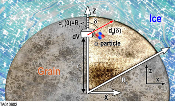
Figure 1. Geometry of the α particle attenuation problem. The dust grain containing the radionuclides is surrounded by ice. A particle is emitted from the volume dV located at a distance rg from the center of the grain. Z is the vertical axis from the center of the grain through dV. The particle is emitted at an angle δ from Z and travels the distance dg(δ).
Download figure:
Standard image High-resolution imageSince irradiation of ice can also produce H2O2 with a yield comparable to the maximum O2 yield (see Section 5), and 0.24% H2O2 would be two orders of magnitude larger than observations, we assessed the effect of grain size on the amount of energy available to the ice mantle following the model described in Appendix A.1. We considered a range of grain radii from 1 to 100 μm. The effect of grain size on radiolytic production is shown in Figure 2. While this effect is low for 1 μm grains (it decreases the available energy by 3.4% only), production is reduced by a factor of 10 for a 100 μm grain. In the case of H2O2, this would still represent an overabundance, an order of magnitude larger than suggested by observations (Bieler et al. 2015).
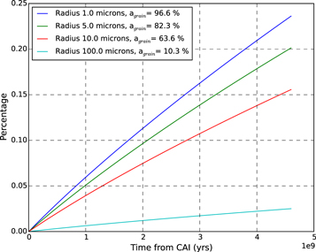
Figure 2. Time evolution of O2 percentage in cometary ice due to radiolysis by α particles, assuming  molec/100 eV, for various grain sizes. For each grain radius, agrain is the percentage of the emitted radiation that exits the grain.
Download figure:
Standard image High-resolution image4.2. Production by -particle and -ray Irradiation


Both β particles and γ-rays are decay products of long-lived radionuclides (40K, 232Th,235U,238U) and short-lived radionuclides (26Al and 60Fe). The latter represent a high amount of energy imparted to the cometary ice in the first million years of its existence. Due to the absence of a firm value on the yield in O2 of γ-rays, and the uncertainty on the yield of electrons at energies typical of decay (see Section 2), we ran calculations with values ranging from 0 to 0.5 molecules/100 eV (maximum observed for heavy nuclei) for both radiation types. The energy imparted to ice is deduced from Equation (1).
Figure 3 shows the results of our calculations. The final O2 percentage in the ice exceeds 1% only in the case of the highest yields considered. We also display an example of time evolution of the O2 fraction in Figure 4. Short-lived radionuclides produce the majority of radiolytic O2. The relative contribution of long-lived radionuclides is likely to be even lower if we consider that after the initial heating by short-lived radionuclides, the comet cooled below 100 K, lowering the O2 yield. Therefore, only very high yields, not supported by experimental data, would allow for a radiolytic production able to match the O2/H2O ratio observed at 67P/C-G.

Figure 3. Final percentage of O2 in cometary ice due to radiolysis by β particles and γ-rays, as a function of the yields  and
and  . The values displayed are upper limits since no destruction process is considered.
Download figure:
Standard image High-resolution image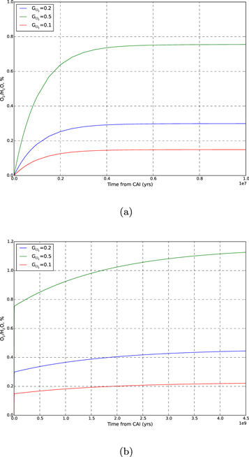
Figure 4. Time evolution of O2 percentage in ice, examples with  values of 0.1, 0.2, and 0.5, and
  . Top panel (a): evolution for the first 10 Myr after CAI, showing mainly the contribution of short-lived radionuclides. Bottom panel (b): evolution for 4.5 Gyr after CAI. The long-lived radionuclides contribute about half as much O2 as the short-lived ones. This contribution assumes no loss in yield due to the cooling of the comet.
Download figure:
Standard image High-resolution image5. Discussion
The values of yield required to eventually reach a concentration of 1%, coupled with experimental evidence, lead to the conclusion that endogenic radiolysis is unlikely to account for the quantities of O2 observed at 67P/C-G. It is therefore more likely that O2 was already present in the material that formed the comet, possibly after being produced in the interstellar cloud Taquet et al. (2016). Endogenic radiolysis could nonetheless have contributed several tenths of percent, which would have to be considered when investigating possible sources for the steady emission of O2. This contribution cannot be precisely quantified using the current state of knowledge on ice radiolysis. Additional experimental data on ice irradiation by particles and γ-rays in the range of energies emitted by radionuclide decay are required.
Another product of ice radiolysis is H2O2; measured yields range between 0.1 and 0.6 molec/100 eV (Teolis et al. 2017). Observations from ROSINA (Bieler et al. 2015) show an H2O2 abundance of at most 0.0023%. From Figure 2, it follows that quantities of H2O2 one to two orders of magnitude (depending on dust grain size) higher than suggested by observations would have been produced in 67P/C-G by α particles alone. The H2O2 saturation dose (steady-state H2O2 concentration reached by an ice sample under constant irradiation) experimentally observed for projectiles of comparable stopping powers is compatible with such a production (Teolis et al. 2017, Figure 8). Additional production by β and γ radiation is harder to quantify. H2O2 saturation doses reached under high-energy electron irradiation is lower than with atomic nuclei irradiation (Teolis et al. 2017). This could indicate that β and γ irradiation would have a lower H2O2 yield than α particles.
The suppression of H2O2 formation due to temperatures above 100 K (Teolis et al. 2017) is unlikely. Mousis et al. (2017) showed that the outer layer of 67P/C-G (several kilometers), to conserve the volatiles observed by Rosetta, would need to have stayed below 100 K for most of the comet's history. Therefore, the part of the comet at the origin of the observations has been under thermal conditions favorable to H2O2 production. Another possible factor in suppressing H2O2 production is that high-energy radiation may have a lower yield than predicted from stopping power alone. Alternatively, H2O2 could have been destroyed by a chemical process yet to be determined. Calculations with the Vienna Ab Initio Simulation package (VASP) (Kresse & Furthmüller 1996) show that H2O2 is stabilized within the ice matrix with an energy of −1.4 eV, to be compared with −0.3, −0.5, −1.1, −1.2 eV for O2, S2, OH, and HO2, respectively. This makes it relatively stable and unlikely to diffuse over a long time period, i.e., until it is destroyed by chemical processes. Among them is a multiple process, globally referred to as dismutation (Dulieu et al. 2017):

Ending up with O2 production, this mechanism has been considered as a possible source for the O2 observed at comet 67P. However such processes would have to be more than 98% efficient to reduce even a H2O2 abundance of 0.1% to the observed value. The outcome of the full chemical network inside the ice critically depends on the activation barriers, which are currently under investigation using first principle solid-state methodology.
On the other hand, experimental yields for the considered range of energies are needed to quantify more accurately how much H2O2 would be expected, and narrow down the cause of its near absence in 67P/C-G.
Here we have considered a radionuclide abundance in the comet based on ordinary chondritic values, for all our calculations. The possibility of inhomogeneities of short-lived radionuclides produced in the protosolar disk has been raised (Lee et al. 1998), which could lead to a comet enriched or impoverished in radionuclides. However, the alternate scenario of supernova injection, an efficient mechanism to enrich the PSN in radionuclides, involves extensive mixing of radionuclides into the disk (Ouellette et al. 2009) and would not lead to significant inhomogeneities.
The radiolytic production per unit of volume can be influenced by the size of the body in which it occurs, only if its dimensions are shorter than the typical radiation range. This could have been the case for the building blocks of the comet shortly after CAI, when short-lived radionuclides were most active. Most of their radiation energy would become available for radiolytic production once the boulders become meter-sized. The accretion scenario of Davidsson et al. (2016), even though its timescale is considerably longer compared to the original scenario of Weidenschilling (1997), yields meter-sized boulders within 0.56 Myr after CAI, at most. This delay is insufficient to fully negate the production by short-lived radionuclides (see Figure 4).
Overall, endogenic radiolysis is unlikely to have produced more than a fraction of the O2 observed in 67P/C-G. Better experimental constraints on the radiolytic production of O2, as well as its subsequent emission, are required for a more definitive assessment of this fraction. Additionally, we have investigated the potential production of H2O2, where our model yields a much higher final abundance (about 0.1%) than that observed by Rosetta (upper limit of 0.0023%). A better understanding of H2O2 production yields and of activation barriers in its dismutation is required to understand how the thermal and/or chemical history parameters led to the comet's present-day composition.
Plots were drawn with Matplotlib (Hunter 2007). This work is supported by the Cassini Project through JPL subcontract 1405853 and by the Rosina project through JPL subcontract 1296001. O.M. acknowledges support from CNES. O.M. and T.R. acknowledge support from the A*MIDEX project (n° ANR-11-IDEX-0001-02) funded by the "Investissements d'Avenir" French Government program, managed by the French National Research Agency (ANR).
Appendix: Appendix Information
A.1. Attenuation of Particles Exiting a Grain

A radionuclide type s inside a dust grain emits, in the form of emission j, a power dPs,j/dV per unit of volume. "Emission j" designates a given emission in the decay chain (e.g., the 5.013 MeV α particle emission from the 231Pa to 227Ac transition in the 235U decay chain). dPs,j/dV is given by:

where ns is the density of radionuclides in the grain (atoms per unit of volume, deduced from the mass fractions in chondrites shown in Table 1, the grain density and the molar masses of the radionuclides), τs is the average decay time of radionuclide s (deduced from the half-life values in Table 1), E0,j is the energy of emission j, and Ij is the absolute intensity of emission j (i.e., the probability of emission j occurring per decay). ns is a function of the time t elapsed since CAIs:

where ns,0 is ns at the time of CAIs.
A small element of volume dV, situated at a distance rg from the center of the grain, emits a power dPs,j isotropically (see Figure 1). We define a z-axis along the radius of the grain passing through dV. Depending on the direction of the emission (angle δ between the trajectory of the radiation and the z-axis), the radiation will travel a distance dg(δ, rg) in the grain before exiting. It will undergo an attenuation following the relationship (Dzaugis et al. 2015):

where Ej(dg) is the energy of the particle after traveling dg, Rstop,j is the stopping distance of particle j in the medium constituting the grain, and bj is a coefficient determined empirically and dependent on the particle type, energy, and the medium considered.
To obtain values of bj and Rstop,j, we used the SRIM-TRIM suite9 (Ziegler et al. 2010). Through a quantum mechanical treatment of ion-atom collisions, SRIM-TRIM calculates the motion of a particle through a user-defined medium. Each run consisted of 100,000 α particles traveling along the x-axis and hitting a target made of either ice (density of 0.94 g cm−3) or fayalite (Fe2SiO4), used as a proxy for comet dust grains (Engrand et al. 2016) with a density of 3.0 g cm−3. The range of the particle is given by the average length it travels along the direction of emission before stopping. We assumed here a straight propagation of the radiation. Though α particles get deviated by elastic collisions, SRIM-TRIM simulations show that at the high energies considered (4–6 Mev), the lateral deviation is noticeably shorter than the distance traveled along the direction of emission (on average 5% of the penetration depth). We find 4 MeV α particles have average Rstop values of 28.8 and 15 μm in ice and fayalite, respectively, while 6 MeV α particles reach ranges of 52.2 and 26.5 μm in these two media.
The coefficient bj is similarly determined by fitting Equation (5) to the loss of energy of the simulated particles. We find the initial part of the trajectory is best fit with bj = 1.2. Since most of the energy is lost in the first half of the particle's travel, we elect to use bj = 1.2 to adequately represent the rate of energy loss in the grain.
The power is emitted isotropically, which allows us to put dPs,j, the power due to radiation s, j emitted by dV, under the form

Now taking into account attenuation, the power  coming out of the grain due to radiation s, j emitted by element dV is

The total power due to radiation s, j coming out of the grain, after integration over dV, is given by
To perform the calculation, the explicit dependence of dg on δ and rg is required.
To do so, we define a Cartesian referential as shown in Figure 1.
The trigonometric functions of δ give us


it follows that:


By putting Equations (11) and (12) to the square, adding them together and using  we get

which leads to

allowing one to perform numerically the integration in Equation (8) and obtain  .
.
A.2. Determination of the Ratios of Stopping Powers
The values of Si commonly used are ratio of mass stopping powers; it is the case in the formula used as a basis for our calculations (Hoffman 1992). The attenuation of a γ-ray beam going through a material can be described by:

where I0 is the original intensity, I(L) is the intensity reaching depth L in the material, μ is the mass stopping power, μl is the attenuation factor and ρ the density of the material (Nelson & Reilly 1991). Si values correspond to a ratio of μ values, while our  values are a ratio of μl values. Equation (15) makes apparent that μl is the inverse of the mean-free-path λ. We calculated, for a 1 MeV beam, values of μ in fayalite and ice using the tables of Storm & Israel (1970). The μ values are respectively 0.027 and 0.031 cm2/g. With densities ρrock = 3.0 g cm−3 and ρwater = 1.0 g cm−3, and using λ = 1/(μρ), we find λ(fayalite) = 12.4 cm and λ(water ice) = 34.6 cm. Using notations related to our case of interest (water versus a "rock" made of fayalite), we can write these relations:
Values of μ are tabulated for individual elements (Storm & Israel 1970). The mass stopping power of compound materials is given by (Nelson & Reilly 1991):

where μj is the μ value of the element j, and wj is its mass fraction in the compound.
We calculated Sγ from the tabulated values of Storm & Israel (1970) for water ice and olivine, for 1 MeV γ-rays; we find Sγ = 1.15, and  .
.
Similarly, we calculated  and
and  through the ratios of their average range in water ice and olivine. We obtained these ranges through SRIM-TRIM and CASINO calculations, for α particles at 4 MeV and electrons at 500 keV, respectively. We find
  and
and  .
.