


Abstract
We present optical spectroscopic and photometric observations of the nearby type Ic supernova (SN Ic) SN 2014L. This SN was discovered by the Tsinghua-NAOC Transient Survey (TNTS) in the nearby type-Sc spiral galaxy M99 (NGC 4254). Fitting to the early-time light curve indicates that SN 2014L was detected at only a few hours after the shock breakout, and it reached a peak brightness of MV = −17.73 ± 0.28 mag (L = [2.06 ± 0.50] ×1042 erg s−1) approximately 13 days later. SN 2014L shows a close resemblance to SN 2007gr in the photometric evolution, while it shows stronger absorption features of intermediate-mass elements (especially Ca ii) in the early-time spectra. Based on simple modeling of the observed light curves, we derived the mass of synthesized 56Ni as MNi = 0.075 ± 0.025 M⊙, and the mass and total energy of the ejecta as Mej = 1.00 ± 0.20M⊙ and Eej = 1.45 ±0.25 foe, respectively. Given these typical explosion parameters, the early detection, and the extensive observations, we suggest that SN 2014L could be a template sample for the investigation of SNe Ic.
Export citation and abstract BibTeX RIS
1. Introduction
Type Ic supernovae are characterized by the absence of hydrogen and helium in the spectra (see, e.g., reviews by Filippenko 1997; Modjaz et al. 2014; Liu et al. 2016; Branch & Wheeler 2017). The primary spectral distinction between regular Ic and Ib is the strength and evolution of helium lines. Recent studies show, however, that weak helium absorptions can be detected in some SNe Ic (Chen et al. 2014; Milisavljevic et al. 2015), while there are also arguments that the helium features are not present in SNe Ic (i.e., Liu et al. 2016). Theoretically, the appearance of helium in the spectra may not necessarily suggest a classification of an SN Ib, which might relate to the abundance ratio of nickel and helium in the outer layers (Wheeler et al. 1987; Shigeyama et al. 1990; Hachisu et al. 1991).
Observationally, SNe Ic are found to show large varieties in spectral features and line profiles. For example, the subclass of broad-lined SNe Ic (BL-Ic) are characterized by broad, highly blueshifted line profiles in their spectra, relatively high luminosity, and considerable kinetic energies of (2–5) × 1052 erg (Woosley & Bloom 2006). Some BL SNe Ic are found to be associated with long-duration gamma-ray bursts (GRBs), e.g., SN 1998bw (Galama et al. 1998; Iwamoto et al. 1998) and SN 2003dh (Hjorth et al. 2003; Mazzali et al. 2003), and their progenitors are reported to have relatively low metallicity (e.g., Woosley et al. 1993; Woosley & Bloom 2006). On the other hand, there are some peculiar SNe Ic events with prominent calcium features and fast spectral evolution, i.e., SN 2012hn (Valenti et al. 2014), which are dubbed as Ca-rich SNe Ic. This observed diversity of SNe Ic indicates that they may arise in different channels, e.g., single massive stars or binary system.
Photometric and spectroscopic observations have been published for dozens of SNe Ic (Bianco et al. 2014; Modjaz et al. 2014). However, the sample with very early observations and good phase coverage (e.g., SN 1994I, Wheeler et al. 1994; Filippenko et al. 1995; Richmo et al. 1996; SN 2007gr, Valenti et al. 2008; Hunter et al. 2009; Chen et al. 2014; SN 2013ge, Drout et al. 2016) is still limited. In this paper, we present the extensive photometric and spectroscopic observations of the nearby SN Ic SN 2014L, spanning from ∼−10 days to ∼140 days relative to the maximum light. This SN was detected at only a few hours after the shock breakout and might be one of the youngest SN Ic ever discovered.
This paper is organized as follows. Observation and data reductions are described in Section 2. The results from photometry and spectroscopy are presented in Sections 3 and 4, respectively. Explosion parameters are calculated and discussed in Section 5. A summary is given in Section 6.
2. Observations
SN 2014L was discovered by the Tsinghua—NAOC (National astronomical observatories of China) transient survey (TNTS) on 2014 January 26.83 UT (Zhang et al. 2014b) in the nearby Sc-type galaxy M99 (=NGC 4254), at an unfiltered magnitude of 17.2. This survey uses a 0.6 m Schmidt telescope (+4K × 4K CCD) located at Xinglong Observatory in China (Zhang et al. 2015). K. Itagaki reported a pre-discovery detection of this transient (with an unfiltered magnitude of 17.9), obtained on 2014 January 24.85 UT with a 0.5 m reflector at the Takamizawa station, Japan. The coordinates of this transient is R.A. = 12h18m48 68 and decl. = +14°24'43
 5 (J2000), locating at 138 west and 159 south of the center of the host galaxy. The latest distance measurement of M99 reported by Tully et al. (2013) as 13.9 ± 1.5 Mpc based on the Tully–Fisher relation is adopted in this paper. This result well matches an alternative distance reported by Poznanski et al. (2009) as 14.4 ± 2.0 Mpc via the expanding photosphere method.
SN 2014L was independently classified as a young SN Ic by several groups (e.g., Akitaya et al. 2014; Li et al. 2014; Ochner et al. 2014; Zhang & Wang 2014) within 1–2 days after the discovery. We thus triggered the follow-up observation campaign on the Li-Jiang 2.4 m telescope (LJT; Fan et al. 2015) with YFOSC (Yunnan Faint Object Spectrograph and Camera; Zhang et al. 2014a) at Li-Jiang Observatory of Yunnan Observatories (YNAO) and the Tsinghua-NAOC 0.8 m telescope (TNT; Wang et al. 2008; Huang et al. 2012) at Xing-Long Observatory NAOC. This campaign spans from t ≈ −10 days to t ≈ +140 days, or from τ ≈ +3 days to τ ≈ +150 days (parameter t denotes to the time relative to the V-band maximum, τ denotes to the time compared to the shock breakout in this paper) covering the full photospheric phase. The daily observations at the first month after shock breakout makes SN 2014L an excellent object for studying the observed properties of SNe Ic.
Figure 1 shows the finder chart and the pre-discovery images of SN 2014L taken by the HST Wide-Field Planetary Camera 2 (WFPC2) on Jan, 2009 under HST program GO-11966 (PI: Regan). At the distance of D = 13.9 ± 1.5 Mpc, the corresponding physical pixel size in the sky is d ∼ 7 pc per pixel. In these pre-explosion images, no point-like source can be detected within 02 from the SN position. The apparent brightness of the white circle region is estimated as mF336W = 22.3 ± 4.0 mag, mF606W = 21.1 ± 0.5 mag and mF814W = 20.5 ± 0.6 mag. On the other hand, there are some brighter and bluer sources located not far from the SN position (i.e., ∼06). Given the high star formation rate of M99 (Soria & Wong 2016), the nearby blue sources around the birth place, the larger host extinction of SN 2014L (see the details in Section 3.2), and the strong Balmer emission lines presented in the spectra (see the details in Section 2.2), SN 2014L likely comes from a relatively young stellar environment covered by thick dust and gas.

Figure 1. Left panel: the finder chart of SN 2014L and its local reference, taken by the LJT and YFOSC on 2014 January. The mean FWHM of this combined image is 160 under the scale of 028/pixel. Right panel: the pre-explosion image, corresponding to the black box on the left panel and including the birth place region of SN 2014L, taken by Hubble Space telescope Wide-Field Planetary Camera 2 in 2009 in the filters of F336W, F606W, and F814W under the scale of 01/pixel. The combined image is also shown. The circles having radii of 02, 06 and 16, respectively, are centered at the location of SN.
Download figure:
Standard image High-resolution image
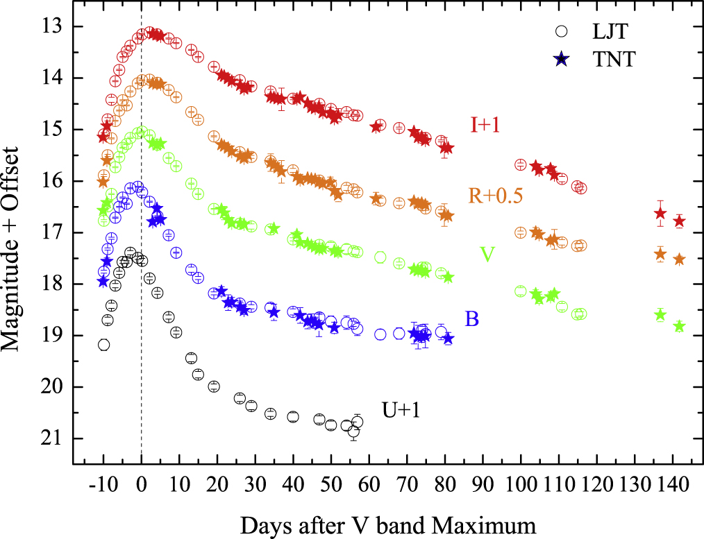
Figure 2. UBVRI light curves of SN 2014L obtained at the Li-Jiang 2.4 m telescope and BVRI light curves obtained at the Tsinghua-NAOC 0.8 m telescope. An offset has been added for better visibility.
Download figure:
Standard image High-resolution image2.1. Photometry
SN 2014L is well-observed in the standard Johnson UBV and Kron–Cousins RI bands, with a typical FWHM 16 for LJT images, and 25 for the TNT images. High-quality template images were taken with the LJT+YFOSC and TNT at 2–3 years after the explosion. We perform background subtraction to remove the time-invariant background structures and better reveal the time-variant SN signals. The photometry of this SN is transformed into the standard Johnson–Cousin photometry system (as listed in Table 1 and presented in Figure 2) through some local standard stars, as marked in the left panel of Figure 1. The UBVRI magnitudes of these reference stars (as listed in Table 2) are calibrated via observing a series of Landolt (1992) photometric standard stars on three photometric nights.
Table 1. UBVRI band Photometry of SN 2014L
| Date | MJD | Daya | U(mag) | B(mag) | V(mag) | R(mag) | I(mag) | Telescope |
|---|---|---|---|---|---|---|---|---|
| Jan 27 | 56684.72 | −10.09 | ⋯ | 17.95(0.06) | 16.57(0.02) | 16.52(0.03) | 16.15(0.03) | TNT |
| Jan 27 | 56684.90 | −9.91 | 18.18(0.11) | 17.76(0.03) | 16.77(0.02) | 16.39(0.02) | 16.09(0.03) | LJT |
| Jan 28 | 56685.74 | −9.07 | ⋯ | 17.56(0.07) | 16.42(0.02) | 16.10(0.03) | 15.93(0.03) | TNT |
| Jan 28 | 56685.91 | −8.90 | 17.70(0.06) | 17.32(0.02) | 16.49(0.01) | 16.00(0.02) | 15.80(0.03) | LJT |
| Jan 29 | 56686.92 | −7.89 | 17.42(0.05) | 17.11(0.02) | 16.25(0.01) | 15.67(0.01) | 15.42(0.05) | LJT |
| Jan 30 | 56687.90 | −6.91 | 17.03(0.04) | 16.71(0.01) | 15.73(0.01) | 15.33(0.01) | 15.06(0.01) | LJT |
| Jan 31 | 56688.95 | −5.86 | 16.78(0.03) | 16.50(0.01) | 15.53(0.01) | 15.13(0.01) | 14.84(0.01) | LJT |
| Feb 01 | 56689.89 | −4.92 | 16.57(0.03) | 16.32(0.01) | 15.35(0.01) | 14.93(0.01) | 14.59(0.01) | LJT |
| Feb 02 | 56690.94 | −3.87 | 16.57(0.02) | 16.44(0.01) | 15.28(0.01) | 15.03(0.01) | 14.48(0.03) | LJT |
| Feb 03 | 56691.87 | −2.94 | 16.39(0.04) | 16.14(0.01) | 15.16(0.01) | 14.76(0.01) | 14.37(0.01) | LJT |
| Feb 05 | 56693.90 | −0.91 | 16.49(0.03) | 16.11(0.01) | 15.07(0.01) | 14.60(0.01) | 14.23(0.01) | LJT |
| Feb 06 | 56694.95 | 0.14 | 16.55(0.05) | 16.22(0.05) | 15.04(0.01) | 14.54(0.01) | 14.15(0.01) | LJT |
| Feb 08 | 56696.96 | 2.15 | 16.89(0.03) | 16.40(0.01) | 15.11(0.01) | 14.53(0.01) | 14.11(0.01) | LJT |
| Feb 09 | 56697.79 | 2.98 | ⋯ | 16.79(0.05) | 15.26(0.01) | 14.60(0.02) | 14.14(0.02) | TNT |
| Feb 10 | 56698.87 | 4.06 | ⋯ | 16.53(0.05) | 15.30(0.01) | 14.61(0.02) | 14.16(0.02) | TNT |
| Feb 11 | 56699.01 | 4.20 | 17.17(0.03) | 16.68(0.01) | 15.29(0.01) | 14.59(0.01) | 14.15(0.01) | LJT |
| Feb 11 | 56699.87 | 5.06 | ⋯ | 16.75(0.05) | 15.27(0.01) | 14.62(0.02) | 14.19(0.02) | TNT |
| Feb 14 | 56702.00 | 7.19 | 17.64(0.04) | 17.05(0.02) | 15.55(0.01) | 14.73(0.01) | 14.23(0.01) | LJT |
| Feb 15 | 56703.99 | 9.18 | 17.94(0.03) | 17.39(0.01) | 15.71(0.01) | 14.87(0.01) | 14.32(0.01) | LJT |
| Feb 19 | 56707.94 | 13.13 | 18.44(0.07) | 17.72(0.05) | 16.05(0.01) | 15.16(0.01) | 14.45(0.01) | LJT |
| Feb 21 | 56709.75 | 14.94 | 18.76(0.06) | 17.88(0.03) | 16.25(0.01) | 15.31(0.03) | 14.59(0.01) | LJT |
| Feb 25 | 56713.89 | 19.08 | 18.99(0.05) | 18.18(0.03) | 16.54(0.01) | 15.63(0.01) | 14.78(0.01) | LJT |
| Feb 02 | 56715.89 | 21.08 | ⋯ | 18.14(0.09) | 16.55(0.02) | 15.79(0.03) | 14.94(0.02) | TNT |
| Feb 28 | 56716.64 | 21.83 | ⋯ | ⋯ | 16.62(0.13) | 15.82(0.05) | 14.96(0.04) | TNT |
| Mar 01 | 56717.65 | 22.84 | ⋯ | 18.36(0.15) | 16.75(0.03) | 15.86(0.04) | 15.01(0.03) | TNT |
| Mar 02 | 56718.62 | 23.81 | ⋯ | 18.35(0.09) | 16.82(0.02) | 15.93(0.03) | 15.06(0.03) | TNT |
| Mar 04 | 56720.72 | 25.91 | 19.22(0.06) | 18.38(0.05) | 16.83(0.02) | 15.94(0.02) | 15.04(0.01) | LJT |
| Mar 04 | 56720.87 | 26.06 | ⋯ | 18.44(0.08) | 16.82(0.03) | 16.02(0.03) | 15.14(0.02) | TNT |
| Mar 05 | 56721.85 | 27.04 | ⋯ | 18.51(0.08) | 16.84(0.02) | 16.06(0.02) | 15.21(0.02) | TNT |
| Mar 06 | 56722.85 | 28.04 | ⋯ | ⋯ | ⋯ | 15.99(0.04) | 15.18(0.03) | TNT |
| Mar 07 | 56723.79 | 28.98 | 19.37(0.07) | 18.44(0.04) | 16.88(0.05) | 16.03(0.03) | 15.16(0.01) | LJT |
| Mar 12 | 56728.84 | 34.03 | 19.52(0.05) | 18.46(0.08) | 16.94(0.06) | 16.11(0.04) | 15.26(0.04) | LJT |
| Mar 12 | 56728.85 | 34.04 | ⋯ | ⋯ | ⋯ | 16.14(0.17) | 15.36(0.04) | TNT |
| Mar 13 | 56729.71 | 34.90 | ⋯ | 18.55(0.16) | 16.92(0.04) | 16.19(0.04) | 15.38(0.04) | TNT |
| Mar 14 | 56730.71 | 35.90 | ⋯ | ⋯ | ⋯ | 16.24(0.06) | 15.40(0.03) | TNT |
| Mar 15 | 56731.71 | 36.90 | ⋯ | ⋯ | ⋯ | 16.32(0.22) | 15.41(0.22) | TNT |
| Mar 18 | 56734.75 | 39.94 | 19.58(0.08) | 18.54(0.06) | 17.13(0.03) | 16.29(0.04) | 15.40(0.02) | LJT |
| Mar 19 | 56735.76 | 40.95 | ⋯ | ⋯ | 17.04(0.06) | 16.41(0.04) | 15.41(0.03) | TNT |
| Mar 20 | 56736.65 | 41.84 | ⋯ | 18.61(0.15) | 17.19(0.03) | 16.48(0.05) | 15.37(0.03) | TNT |
| Mar 22 | 56738.61 | 43.80 | ⋯ | 18.73(0.14) | 17.21(0.02) | 16.44(0.04) | 15.48(0.03) | TNT |
| Mar 23 | 56739.62 | 44.81 | ⋯ | 18.71(0.13) | 17.25(0.04) | 16.46(0.04) | 15.57(0.03) | TNT |
| Mar 24 | 56740.62 | 45.81 | ⋯ | 18.75(0.11) | 17.28(0.04) | 16.47(0.04) | 15.59(0.03) | TNT |
| Mar 25 | 56741.62 | 46.81 | ⋯ | 18.79(0.23) | 17.32(0.04) | 16.52(0.07) | 15.55(0.04) | TNT |
| Mar 25 | 56741.69 | 46.88 | 19.63(0.07) | 18.65(0.06) | 17.24(0.03) | 16.49(0.02) | 15.50(0.02) | LJT |
| Mar 26 | 56742.62 | 47.81 | ⋯ | ⋯ | 17.31(0.05) | 16.55(0.05) | 15.67(0.03) | TNT |
| Mar 28 | 56744.62 | 49.81 | ⋯ | ⋯ | ⋯ | 16.53(0.11) | 15.68(0.06) | TNT |
| Mar 28 | 56744.76 | 49.95 | 19.74(0.08) | 18.73(0.11) | 17.27(0.08) | 16.56(0.05) | 15.60(0.03) | LJT |
| Mar 29 | 56745.63 | 50.82 | ⋯ | 18.85(0.11) | 17.35(0.03) | 16.69(0.04) | 15.79(0.04) | TNT |
| Mar 30 | 56746.64 | 51.83 | ⋯ | ⋯ | 17.38(0.09) | 16.77(0.13) | 15.72(0.13) | TNT |
| Apr 01 | 56748.84 | 54.03 | 19.75(0.09) | 18.75(0.13) | 17.32(0.09) | 16.63(0.05) | 15.66(0.02) | LJT |
| Apr 03 | 56750.71 | 55.90 | 19.86(0.18) | 18.77(0.05) | 17.36(0.06) | 16.66(0.04) | 15.72(0.02) | LJT |
| Apr 04 | 56751.72 | 56.91 | 19.68(0.15) | 18.87(0.13) | 17.38(0.06) | 16.72(0.04) | 15.73(0.01) | LJT |
| Apr 09 | 56756.63 | 61.82 | ⋯ | ⋯ | ⋯ | 16.84(0.12) | 15.95(0.05) | TNT |
| Apr 10 | 56757.78 | 62.97 | ⋯ | 18.98(0.10) | 17.48(0.11) | 16.88(0.05) | 15.91(0.02) | LJT |
| Apr 15 | 56762.72 | 67.91 | ⋯ | 18.96(0.11) | 17.60(0.03) | 16.93(0.04) | 15.97(0.02) | LJT |
| Apr 19 | 56766.63 | 71.82 | ⋯ | 18.95(0.21) | 17.71(0.05) | 16.89(0.05) | 16.04(0.03) | TNT |
| Apr 20 | 56767.72 | 72.91 | ⋯ | 19.03(0.23) | 17.74(0.06) | 16.94(0.06) | 16.15(0.05) | TNT |
| Apr 21 | 56768.69 | 73.88 | ⋯ | 19.02(0.11) | 17.73(0.04) | 16.93(0.04) | 16.14(0.05) | TNT |
| Apr 21 | 56768.75 | 73.94 | ⋯ | 18.89(0.07) | 17.68(0.04) | 16.97(0.03) | 16.16(0.04) | LJT |
| Apr 22 | 56769.65 | 74.84 | ⋯ | 19.01(0.23) | 17.77(0.06) | 16.96(0.06) | 16.21(0.04) | TNT |
| Apr 22 | 56769.70 | 74.89 | ⋯ | 18.97(0.08) | 17.68(0.07) | 17.03(0.04) | 16.16(0.01) | LJT |
| Apr 26 | 56773.77 | 78.96 | ⋯ | 18.93(0.15) | 17.79(0.05) | 17.09(0.03) | 16.22(0.02) | LJT |
| Apr 27 | 56774.65 | 79.84 | ⋯ | ⋯ | ⋯ | 17.16(0.22) | 16.36(0.20) | TNT |
| Apr 28 | 56775.65 | 80.84 | ⋯ | 19.06(0.12) | 17.87(0.05) | 17.18(0.05) | 16.36(0.05) | TNT |
| May 17 | 56794.72 | 99.91 | ⋯ | ⋯ | 18.14(0.07) | 17.50(0.03) | 16.68(0.03) | LJT |
| May 20 | 56798.70 | 103.89 | ⋯ | ⋯ | 18.19(0.08) | 17.49(0.09) | 16.71(0.05) | TNT |
| May 22 | 56799.61 | 104.80 | ⋯ | ⋯ | 18.29(0.09) | 17.54(0.07) | 16.79(0.06) | TNT |
| May 25 | 56802.64 | 107.83 | ⋯ | ⋯ | 18.25(0.07) | 17.66(0.05) | 16.76(0.06) | TNT |
| May 26 | 56803.64 | 108.83 | ⋯ | ⋯ | 18.19(0.06) | 17.63(0.19) | 16.88(0.07) | TNT |
| May 28 | 56805.63 | 110.82 | ⋯ | ⋯ | 18.44(0.06) | 17.69(0.05) | 16.96(0.05) | LJT |
| Jun 01 | 56809.62 | 114.81 | ⋯ | ⋯ | 18.59(0.05) | 17.76(0.04) | 17.10(0.03) | LJT |
| Jun 02 | 56810.65 | 115.84 | ⋯ | ⋯ | 18.58(0.04) | 17.75(0.04) | 17.14(0.03) | LJT |
| Jun 23 | 56831.57 | 136.76 | ⋯ | ⋯ | 18.60(0.13) | 17.92(0.15) | 17.63(0.25) | TNT |
| Jun 27 | 56836.57 | 141.76 | ⋯ | ⋯ | 18.82(0.10) | 18.02(0.06) | 17.78(0.13) | TNT |
Notes.
aRelative to the V-band maximum, MJD = 56694.81.A machine-readable version of the table is available.
Table 2. The UBVRI band Magnitudes of the Local Photometric Standards in the Field of SN 2014L
| Star | U(mag) | B(mag) | V(mag) | R(mag) | I(mag) |
|---|---|---|---|---|---|
| 1 | 15.05(0.02) | 14.74(0.01) | 14.01(0.02) | 13.62(0.01) | 13.24(0.02) |
| 2 | 19.61(0.04) | 18.56(0.01) | 17.46(0.02) | 16.78(0.02) | 16.17(0.03) |
| 3 | 17.29(0.03) | 17.28(0.02) | 16.67(0.01) | 16.33(0.02) | 15.96(0.02) |
| 4 | 17.51(0.03) | 17.47(0.02) | 16.78(0.01) | 16.41(0.01) | 16.02(0.02) |
| 5 | 14.30(0.02) | 14.11(0.01) | 13.44(0.01) | 13.09(0.02) | 12.73(0.02) |
| 6 | 19.03(0.03) | 17.60(0.01) | 16.28(0.01) | 15.46(0.01) | 14.72(0.01) |
| 7 | 18.36(0.03) | 18.23(0.01) | 17.39(0.02) | 16.93(0.01) | 16.44(0.02) |
Note. See Figure 1 for the finder chart of these reference stars.
A machine-readable version of the table is available.
Download table as: DataTypeset image
2.2. Spectroscopy
Figure 3 shows the spectral sequence of SN 2014L over a period of about four months starting from 2014 January 27. The observation journal of these spectra is listed in Table 3, including 13 spectra from the LJT (+YFOSC) and 1 spectrum from the Xing-Long 2.16 m telescope (XLT) with the BFOSC (Beijing Faint Object Spectrograph and Camera). All of these spectra are calibrated in both wavelength and flux, and they are corrected for telluric absorption and redshift. The narrow emission lines (e.g., Hα, Hβ) presented in the spectra are due to the contamination in the host galaxy, which becomes dominating at late phase. Variations of these narrow emissions are due to the slit position and spectral resolution. Two spectra from the ANU WiFeS SuperNovA Program (AWSNAP; Childress et al. 2016) are also included in this figure to fill the observation gaps.

Figure 3. Spectral series of SN 2014L. The black spectra are from the Li-Jiang 2.4 m telescope, the red one is from the Xi-Long 2.16 m telescope, and the green are from the ANU WiFeS SuperNovA Program. The data used to create this figure are available.
Download figure:
Standard image High-resolution imageTable 3. Journal of Spectroscopic Observations of SN 2014L
| Date | MJD | Epocha | Res. | Range | Exp. Time | Airmass | Telescope |
|---|---|---|---|---|---|---|---|
| (UT) | (days) | (Å) | (Å) | (s) | (+Instrument) | ||
| Jan 27 | 56684.81 | −10.00 | 3700–8700 | 16 | 3000 | 1.13 | XLT+BFOSC |
| Jan 27 | 56684.91 | −9.90 | 3380–9150 | 18 | 2100 | 1.04 | LJT+YFOSC |
| Jan 28 | 56685.91 | −8.90 | 3520–9130 | 18 | 2400 | 1.04 | LJT+YFOSC |
| Jan 30 | 56687.91 | −6.90 | 3520–9130 | 18 | 2100 | 1.04 | LJT+YFOSC |
| Feb 03 | 56691.88 | −2.93 | 3430–9150 | 18 | 1800 | 1.03 | LJT+YFOSC |
| Feb 05 | 56693.90 | −0.91 | 3480–9130 | 18 | 2400 | 1.06 | LJT+YFOSC |
| Feb 19 | 56707.90 | 13.09 | 3520–9100 | 18 | 2400 | 1.15 | LJT+YFOSC |
| Feb 25 | 56713.90 | 19.09 | 3500–9100 | 18 | 2100 | 1.21 | LJT+YFOSC |
| Mar 04 | 56720.72 | 25.91 | 3500–9100 | 18 | 2500 | 1.09 | LJT+YFOSC |
| Mar 25 | 56741.70 | 46.89 | 3520–9100 | 18 | 2700 | 1.04 | LJT+YFOSC |
| Apr 10 | 56757.79 | 62.98 | 3530–9150 | 18 | 3000 | 1.25 | LJT+YFOSC |
| Apr 22 | 56769.76 | 74.95 | 3590–9800 | 50 | 1500 | 1.29 | LJT+YFOSC |
| May 17 | 56794.70 | 99.89 | 3920–9680 | 50 | 1500 | 1.32 | LJT+YFOSC |
| May 28 | 56805.65 | 110.84 | 3690–9210 | 50 | 1800 | 1.21 | LJT+YFOSC |
Note. Spectroscopic observations of SN 2014L.
aRelative to the V-band maximum, MJD = 56694.81.A machine-readable version of the table is available.
Download table as: DataTypeset image
3. Photometric Results
A polynomial fit is applied to the UBVRI band light curves around the maximum light to derive the peak magnitudes, dates, and the post-peak decline rates, as listed in Table 4. For example, SN 2014L reached its V-band peak on MJD = 56694.81, and it reached the peaks at slightly different epochs in other bands. By adopting the distance D = 13.9 ± 1.5 Mpc (as discussed in Section 2) and the total extinction E(B − V) = 0.67 ± 0.11 (derived in Section 3.2), we obtain an absolute V-band peak magnitude of −17.73 ± 0.28 mag for SN 2014L.
Table 4. Absolute Peak Brightness of SN 2014L in UBVRI bands
| Band | tmax | mpeak | Mpeak | Δm15 |
|---|---|---|---|---|
| (MJD-56000) | (mag) | (mag) | (mag) | |
| U | 692.45(0.40) | 16.45(0.04) | −17.54(0.41) | 2.00(0.05) |
| B | 693.16(0.25) | 16.16(0.03) | −17.30(0.35) | 1.60(0.03) |
| V | 694.81(0.20) | 15.06(0.02) | −17.73(0.28) | 1.10(0.03) |
| R | 696.88(0.20) | 14.54(0.02) | −17.71(0.23) | 0.94(0.02) |
| I | 697.33(0.25) | 14.14(0.03) | −17.64(0.19) | 0.56(0.03) |
Download table as: ASCIITypeset image
3.1. Light Curves
Figure 4 displays the UBVRI light curves of SN 2014L compared to those of some typical SNe to better understand the photometric properties of SN 2014L. Three SNe Ic, SN 1994I (Richmo et al. 1996), SN 2007gr (Valenti et al. 2008; Chen et al. 2014), and SN 2004aw (Taubenberger et al. 2006); the board-line SN Ic, SN 1998bw (Clocchiatti et al. 2011); SN Ib, SN 2008D (Modjaz et al. 2009; Tanaka et al. 2009; Bianco et al. 2014); faint and calcium-rich events SN 2005E (Perets et al. 2010) and SN 2012hn (Valenti et al. 2014) are plotted in Figure 4.

Figure 4. Comparison of the UBVRI light curves of SN 2014L with some well-observed SNe Ib/c, including SN 2007gr, SN 1994I, SN 2004aw, SN 1998bw, SN 2008D, SN 2012hn, and SN 2005E. All light curves are normalized to their peaks in each band.
Download figure:
Standard image High-resolution imageThe light curves of SN 2014L are overall similar to those of SN 2007gr, though the former appears slightly narrower than the latter. It is surprising that SN 2014L, SN 2004aw, SN 2007gr, and SN 1998bw show similar evolution in the U band, with a small scatter of <0.2 mag. In the B band, SN 2014L, SN 1994I and SN 2012hn also show similar light-curve evolution at t < +20 days. After that, these SNe exhibit different decay rates. Larger scatters also exist in the VRI bands at similar phases.
These SNe can be divided into three clusters, depending on the decline rate from 0 < t < +30 days. For example, the slow declining group including SN 2004aw, SN BL-Ic 1998bw, SN Ib 2008D; the fast declining group including SN Ic 1994I and SN Ca-rich 2005E; and the intermediate declining group including SN Ic 2014L, SN Ic 2007gr, and SN Ca-rich 2012hn. In each cluster, however, apparent differences can be found in spectral comparisons at both photospheric and nebular phase of Section 4.
The relatively similar peak properties are often in contrast with the considerable spread in the properties of the late-time tail of the light curve (e.g., Wheeler et al. 2015, hereafter is WJC 15). Clear differences existing among the tails of these light curves might be related to the different optical opacities and γ-ray leakage rates of different SNe Ib/c.
3.2. Reddening
The early spectra of SN 2014L show red continuum and significant absorption of narrow Na i D from the host galaxy. These features suggest substantial line-of-sight reddening towards the SN. The equivalent width (EW) of Na i D absorption in the SN spectra can be used to estimate the reddening according to some empirical correlations between reddening and EW of Na i D, e.g., E(B − V) = 0.16 EWNa − 0.01 (Turatto et al. 2003), and E(B − V) = 0.25 EWNa (Barbon et al. 1990). However, these empirical correlations usually exhibit large scatter for the extinction measurement (e.g., Poznanski et al. 2011; Phillips et al. 2013). In SN 2014L, EW(Na i D) is measured as 2.7 ± 0.1 Å, which corresponds to a color excess of E(B − V)host = 0.42 ± 0.04 or 0.68 ± 0.05 following the above relations.
Alternatively, the host-galaxy reddening of SNe Ib/c can be estimated by a photometric method. Based on a larger sample of SNe Ib/c, Drout et al. (2011) found that the V − R color of extinction-corrected SNe Ib/c is tightly clustered at 0.26 ± 0.06 mag at t ≈ +10 days after the V-band maximum, and 0.29 ± 0.08 mag at t ≈ +10 days after the R-band maximum. This method yields an estimate of E(B − V)total = 0.75 ± 0.05 mag for SN 2014L assuming an RV = 3.1 Milky Way extinction law for the host galaxy. Adopting the Galactic extinction E(B − V)Gal = 0.04 ± 0.01 (Schlafly & Finkbeiner 2011), the host reddening derived from the V − R color is E(B − V)host = 0.71 ± 0.05 mag.
Combining the estimations obtained from Na i D absorption and V − R color, an average value of the total reddening, E(B − V) = 0.67 ± 0.11 mag, is adopted in this paper.
3.3. Color Curves
The reddening-corrected color curves of SN 2014L are displayed in Figure 5, together with those of the comparison sample shown in Figure 4. The B − V color of SN 2014L is similar to that of SN 1998bw, SN 2008D, and SN 2007gr, but the difference exists in other bands, especially at t > +20 days relative to the V-band maximum. The scatter shown before the peak can be attributed to the difference in temperature and metal abundance of the outer ejecta, while the scatter seen after t ≈ +20 days could be related to the duration of photospheric phase.

Figure 5. Comparison of the color curves among SN 2014L, SN 2007gr, SN 2012hn, SN 1998bw, SN 2004aw, SN 1994I, and SN 2008D. All of these curves are corrected for the reddening due to the Milky Way and Host galaxies.
Download figure:
Standard image High-resolution imageThe large scatter among the colors of these SNe, even in the SNe Ib/c group, might not suggest a uniform color evolution for these SNe. However, as mentioned before, there seems to exist an intrinsic V − R color for regular SNe Ib/c at about ten days after the peak (Drout et al. 2011). Such an inherent color distribution might also exist in B − V and V − I color at a similar phase in Figure 4.
3.4. Quasi-bolometric Light Curve
Figure 6 displays the quasi-bolometric light curves of our sample, based on the UBVRI photometry presented in Figure 4. SN 2014L researches the peak quasi-bolometric luminosity of L = (2.06 ± 0.50) × 1042 erg s−1 at MJD = 56693.86, which is about one day earlier than the V-band maximum. The fractional contribution of the ultraviolet (UV) and near-infrared (NIR) emission to the bolometric luminosity can be ∼30%–40% at around the peak for SNe Ib/c (e.g., ∼40% in SN 2008D; Modjaz et al. 2009). Considering the missed UV and NIR flux of SN 2014L, the total bolometric flux of this SN could reach ∼3 × 1042 erg s−1 around the peak.

Figure 6. UBVRI quasi-bolometric light curves of SN 2014L, SN 2007gr, SN 2005E, SN 2012hn, SN 1998bw, SN 2004aw, SN 1994I, and SN 2008D.
Download figure:
Standard image High-resolution image4. Spectral Evolution
The spectral sequence of SN 2014L, covering the full evolution at the photospheric and a part of the early nebular phase, was exhibited in Figure 3. A closer comparison between SN 2014L and other representative SNe Ib/c are presented at four selected phases as plotted in Figure 7. All of these spectra have been corrected for redshifts and reddening.

Figure 7. Spectral comparison among SN 2014L, SN 2007gr, SN 2005E, SN 2012hn, SN 1998bw, SN 2004aw, SN 1994I, and SN 2008D at four selected phases. The positions of major line features are marked by dashed-lines referring to the spectral identification of SN 2007gr (Valenti et al. 2008; Hunter et al. 2009; Chen et al. 2014). The spectra in panel (d) are normalized to the flux at around 7300 Å and vertically shifted for better visibility.
Download figure:
Standard image High-resolution image4.1. Early Phase
The early-time spectra (i.e., at a few days after the explosion) contain prominent features to distinguish it among different subclasses of SNe. Figure 7(a) shows the t ∼ −7 day spectra of SN 2014L and some comparison SNe Ib/c including SN 2007gr (Chen et al. 2014), SN 1994I (Filippenko et al. 1995), SN 2004aw (Modjaz et al. 2014), SN 1998bw (Patat et al. 2001), and SN 2008D (Modjaz et al. 2009). Compared to the almost featureless spectrum of SN 2004aw and the board-lined spectrum of SN 1998bw, the spectra of SN 2014L, SN 2007gr, and SN 1994I are characterized by the absorptions of some intermediate-mass elements (IMEs, e.g., Ca, Si, O, and C) and Fe ii. The clear absorption near 6150 Å in the spectra of SN 2014L, SN 2007gr, and SN 1994I can be identified as the feature of Si ii λ6355. The absorption near about 5600 Å is likely attributed to the absorption of Na i D rather than He i λ5876 because of the absence of other helium lines as found in the spectrum of SN Ib 2008D. Overall, SN 2014L shows close resemblances to SN 2007gr and SN 1994I, except that it has more prominent absorption features of Ca ii NIR triplet. The difference in absorptions of Ca ii NIR triplet might indicate difference at the outer layer of ejecta, as discussed in Section 4.5.
4.2. Around Maximum
At around the maximum, the spectral features of SN 2014L are very similar to those of SN 2007gr. These two SNe Ic show narrower absorptions of Si, O, Na, and Fe than SN 1994I and SN 2004aw. In particular, SN 2014L seems to have unusually strong absorption features for a Ca ii NIR triplet, comparable to that of the Ca-rich events such as SN 2005E (Perets et al. 2010) and SN 2012hn (Valenti et al. 2014). The strong Ca ii NIR triplet in SN 2014L might relate to the abundance enrichment of IMEs at the outer layer. To investigate the relative abundance of Si, Ca, and O measured from the spectra shown in Figure 7(b), we plot the EW ratio of O i λ7774/Ca ii NIR triplet versus Si ii λ6355/Ca ii NIR triplet in Figure 8. One can see that the absorption lines ratio Ca/O of SN 2014L is close to that of SN 1994I, while the Ca/Si ratio of SN 2014L is similar to that of SN 2007gr. Both of these two ratios measured from SN 2014L are smaller than the calcium-rich events like SN 2005E and SN 2012hn, ruling out the calcium-rich subclass. Nevertheless, the synthetic spectra at around maximum by (Iwamoto et al. 1998) suggests that the strength of Ca ii NIR triplet is weaker than that of Si ii and O i.

Figure 8. The EW ratio of O i λ7774 and Ca ii NIR triplet is plotted vs. that of Si ii λ6355 and Ca ii NIR triplet for sample shown in Figure 7. The arrow symbol represents the region expected for SN 1998bw. The size of each symbol is related to the estimated uncertainties.
Download figure:
Standard image High-resolution imageCompared to other subclasses of SNe Ib/c, the BL SNe Ic tend to cluster at the top right region of Figure 8. Note, however, that it is hard to measure the absorptions of Ca ii NIR triplet and O i λ7774 in the spectra of SN 1998bw because these two features are blended before and near the maximum light. Moreover, these absorptions cover the wavelength range of the high-velocity Ca ii NIR triplet and the photospheric components of Ca ii NIR triplet and O i λ7774.
According to the distributions shown in Figures 8 and 6, we can divide our sample of SNe Ib/c into three groups. For example, SN 2005E and SN 2012hn had lower luminosity and are located at the bottom of Figure 8. The SN 1998bw-like objects tend to have a smaller amount of calcium and higher luminosity, while the remaining SNe Ib/c in our sample have a moderate luminosity and lie in the center of Figure 8. Of the selected sample, SN 2004aw can be regarded as the transitional event linking the BL SNe Ic with the ordinary ones. The distribution of SNe Ic in Figures 8 and 6 suggests that the relative strength of Ca ii NIR triplet measured in the near-maximum spectra is inversely related to their peak luminosities. Namely, SNe Ic with a significant amount of calcium tend to have lower luminosities. This result may still suffer from small-number statistics, but it is consistent with the theoretical prediction that the O/Ca ratio increases with the mass of progenitor for core-collapse SNe (Houck & Fransson 1996). Thus, a comparable O/Ca ratio seen in SN 2014L, SN 1994I, and SN 2007gr might imply that they have similar progenitor masses and brightness, while SN 2004aw and SN 1998bw are likely from more massive progenitors. It is possible that the Ca-rich events might have lower-mass progenitor systems given the fact that they tend to occur at positions far from the host galaxies. However, massive stars could go for an outing through tidal stripping during galaxy interactions. And we can not rule out a massive progenitor scenario for the Ca-rich events thoroughly (Kasliwal et al. 2012).
4.3. One Month after Maximum
By t ∼ 1 month, the spectra show a clear distinction for different SNe Ic, as shown in Figure 7(c). For example, the t ≈ +26 day spectrum of SN 2014L shows a close resemblance to the t ≈ +35 day of SN 2007gr and the t ≈ +26 day spectrum of SN 1994I, while its t ≈ +36 day spectrum shows less photospheric features compared to the t ≈ +35 day spectrum of SN 2007gr. This implies that SN 2014L has a relatively faster spectral evolution than SN 2007gr. In comparison, the Ca-rich class seems to be the most rapidly evolving spectral feature. At this phase, some nebular features, such as the emission at around 7300 Å (due to the blended lines of O ii and Ca ii) started to emerge. The significant differences in the spectral evolution conform to the scatter seen in the color curves at similar phases. This carbon feature becomes unambiguous in the t ∼ 26 day observed spectrum of SN 1994I due to the diffraction fringing effect of the instrument.
It should be noted that the C i λ9087 absorption is detected in the spectra of SN 2014L and SN 2007gr. The presence of such carbon line is not necessarily in the t ∼ 26 day spectrum of SN 1994I due to the diffraction fringing effect of the instrument. However, detection of this C i line was reported in the t ≈ +10 day spectrum of SN 1994I (Baron et al. 1996). The feature of C i observations indicates that SN 2014L, SN 2007gr, and SN 1994I might arise from carbon-rich progenitors (Baron et al. 1996; Valenti et al. 2008).
4.4. Beginning of Nebular Phase
Figure 7(d) displays the spectra of these SNe at the beginning of nebular phase when the spectra of core-collapse SNe are dominated by a few emissions of IMEs (e.g., O, Mg, Ca). For example, the latest spectrum of SN 2014L is dominated primarily by the emission lines [O i] λλ6300, 6364, a blend of [Ca ii] λλ7291, 7324 and [O ii] λλ7300, 7330, and the Ca ii NIR triplet. However, some photospheric components (e.g., the absorptions of Na i D, O i λ7774 and Ca ii NIR triplet) are still evident in this phase. Similar features are also found in the spectra of SN 1994I, and SN 2007gr. The BL-Ic SN 1998bw shows similar emissions but contains more photospheric features. It indicates a slower evolution in the broad-lined event.
The spectrum of SN 2012hn at t ≈ +34 days keeps some photospheric features and dominated by the emissions of [Ca ii] λλ7291, 7324 and [O ii] λλ7300, 7330, and the Ca ii NIR triplet. Similar emissions are also found in the spectrum of SN 2005E at t ≈ +53 days with less photospheric components. The difference between Ca-rich event, and SNe Ib/c at the early nebular era is the emission of [O i] λλ6300, 6364 which is very weak in the former. Besides, SN 2005E did not develop clear emission of Mg i] and SN 2012hn develops this feature rather slowly. These imply different progenitor systems or explosion mechanism between SNe Ib/c and Ca-rich events. The spectrum of SN 2012hn at t ≈ +151 days evolved to the later nebular phase is similar to the spectra of SNe Ic at about one year after the explosion. It confirms the fact of fast evolution in Ca-rich events.
The apparent and almost symmetric double-peaked feature is found in the [O i] λλ6300, 6364 emissions of SN 2008D. The trace of double-peaked [O i] might exist in that of SN 2007gr and SN 1998bw. However, it is not clear in the spectra of SN 2014L. These might indicate a different geometric structure of the ejecta.
4.5. Velocities
The ejecta velocities derived by the absorption minima of Ca ii H&K, Na i D, Si ii λ6355, C ii λ6580, O i λ7774, Ca ii NIR triplet, and C i λ9087 of SN 2014L are shown in Figure 9. In the early phase, the Ca ii shows a much higher velocity relative to Na i, Si ii, C ii, and O i, and this discrepancy is similarly seen in type Ia supernovae (i.e., Zhao et al. 2015). This might be due to the fact that Ca ii has relatively lower excitation/ionization energy and it can be formed at more distant regions (higher velocities). At t > +10 days, the velocities of Ca ii, Na i, and O i decline slowly and they all tend to reach a velocity plateau of about 8000–10,000 km s−1. We note that the velocity of Na i D shows a significant increase from 8500 km s−1 to 10000 km s−1 during the period from t ∼ 10 days to t ∼ 20 days. This is seen in some SNe Ic (e.g., Hunter et al. 2009) and might be due to the contributions from other spectral lines (e.g., Na ii or He i λ5876).

Figure 9. Ejecta velocities of SN 2014L, as inferred from absorption minima of Ca ii H&K, Na i D, Si ii λ6355, C ii λ6580, O i λ7774, Ca ii NIR triplet, and C i λ9087.
Download figure:
Standard image High-resolution imageFigure 10 shows the comparison of the velocities inferred from Si ii λ6355 and Ca ii NIR triplet for different SNe Ic, including SN 2014L, SN 2007gr, SN 1994I, and SN 2004aw. One can see that SN 2014L shows a higher Si ii velocity than that of SN 2007gr. Before the maximum light, the velocity of the Ca II lines in SN 2014L exhibits a remarkably high decline rate ∼ 600 km s−1 day −1. The more significant decline rate of Ca ii velocity makes a lower velocity plateau of SN 2014L than the comparison.

Figure 10. Velocity comparison of SN 2014L, SN 2007gr, SN 1994I, and SN 2004aw. Top panel: velocity inferred from absorption minimum of Si ii λ6355; Bottom panel: average velocity inferred from absorption minimum of Ca ii NIR triplet.
Download figure:
Standard image High-resolution image5. Explosion Parameters
Some basic explosion parameters, e.g., synthesized 56Ni mass (MNi), ejecta mass (Mej), and ejecta kinetic energy (Eke) can be estimated from the observed peak flux (Lmax) and rise time (tr) of the bolometric light curve, and the photospheric velocity (vph) around the peak brightness with the assumption of a constant opacity. For example, MNi can be estimated using the Arnett law (Arnett 1982; Stritzinger & Leibundgut 2005):

where, τNi = 8.8 and τCo = 111.3 are the decay time of 56Ni and 56Co.
Besides, following Arnett (1982) and the simplifications in WJC 15, we write:


where κ is the effective optical opacity, vph,9 is the velocity at the photosphere in units of 109 cm s−1.
On the other hand, Mej and Eke can be derived from the late-time tail of the light curves,


where C is a dimensionless structure constant, typically about 0.05, κγ is the gamma-ray opacity, T0 is the gamma-ray trapping timescale (as defined in Clocchiatti & Wheeler 1996) and can be derived from the observed later-time light curves (see the details in WJC 15).
Explosion parameters of SN 2014L, SN 1994I, and SN 2007gr are measured and compared at below because they show many similarities in observation.
5.1. Rise Time
The rise time tr is essential to infer the mass of synthesized 56Ni via Equation (1). It can be measured from the very early light curve.
Three groups reported the detection of SN 2014L in their pre-discovery images after the discovery report of Zhang et al. (2014b). The first detection was obtained by Koichi Itagaki (KI) through a 0.5 m reflector telescope at the Takamizawa station on January 24.85 (Yamaoka 2014) in a clear band image (roughly R = 18.15 ± 0.50 mag). Later on, Pan-STARRS1 reported the detection for this SN, marked as PS1-14kd, with the r = 17.01 mag on UT 2014 January 26.49. Gregory Haider (GH) also detected it on January 26.54 in the clear images (roughly R = 17.00 ± 0.40 mag) using the 12.5 inches reflector telescope at Christmas Valley. Combining these pre-discovery detections with the early R-band light curve obtained by LJT and TNT, the shock breakout date of SN 2014L was derived on 2014 January 22.5 (MJD = 56679.5 ± 1.0) through the t2 law approximation of the fireball model, see Figure 11. It suggests that SN 2014L reached its bolometric maximum at about 14.5 days after the shock breakout.

Figure 11. tn fitting for the early observation of SN 2014L. The exponent of different curves are marked.
Download figure:
Standard image High-resolution imageHowever, the fireball model might not be valid in the case of SNe Ic. The physics behind this model is that the increasing internal heating roughly compensates the adiabatic cooling of the ejecta due to Ni-decay. Since the envelope of SNe Ic is shock-heated, the Ni-decay plays less of a role than in it does in the case of SNe Ia (e.g., SNe Ia mag have 5–10 times more nickel than SNe Ic). Thus, the fireball model may not be capable of giving an accurate prediction for the moment of shock breakout. Furthermore, some poor-fit results of the fireball model in the case of very-young SNe Ia would suggest a steeper power-law index (e.g., Zheng et al. 2013, 2014).
We noted that some previous works (e.g., Valenti et al. 2008; Chen et al. 2014; WJC 15) suggested that the rise time of SN 2007gr is about 13–14 days. Given the narrower light curve of SN 2014L, as presented in Figure 4, its rise time might be shorter than that of the SN 2007gr. Moreover, the light-curve modeling in Section 5.3 suggests tr = 13 days of SN 2014L. Meanwhile, we liberalized the exponent of the power law and found a value of 1.4 with a tr = 13 days. Considering the light-curve comparison of SN 2007gr, the following light-curve modeling, and the result of t1.4 fit, we adopted tr = 13 days as the rise time of SN 2014L in the related calculations. The rise time suggests that the shock breakout time of this SN is on 2014 January 24.8 (MJD = 56682.8 ± 1.0). It indicates that the first detection of SN 2014L taken by KI is only a few hours after the shock breakout. Thus, SN 2014L might be the earliest detected SN Ic to date.
5.2. Mass and Energy of the Ejecta
The tr, Lmax, vph, and T0 parameters of SN 2014L, SN 1994I, and SN 2007gr derived from the light curve and spectra are listed in Table 5. A fiducial optical opacity κ = 0.1 cm2 g−1, and a fiducial gamma-ray opacity κγ = 0.03 cm2 g−1 are taken to calculate Mej and Eke. In Table 6, as noted by WJC 15, parameters derived from the peak do not match those arising from the tail. That relates to the fiducial value of κ and κγ adopted in the calculation. If we set the results derived from the peak equal to that from the tail, a relation about κ and κγ can be written as

WJC 15 assumed that κγ is less dependent on explosion parameters than κ. Thus, κ derived from Equation (6), where κγ = 0.03 cm2 g−1, is close to 0.02–0.03 cm2 g−1. This is much smaller than the assumed κ = 0.1 cm2 g−1.
Table 5. Explosion Parameters of Some Well-observed SNe Ic
| SN | tra | Lpeak | vph | T0b |
 c
c
|
|---|---|---|---|---|---|
| (days) | (1042 erg s−1) | (km s−1) | (days) | (M⊙) | |
| 2014L | 13.0 | 2.06 | 7650 | 90 | 0.075 |
| 1994I | 12.0 | 2.63 | 9900 | 85 | 0.089 |
| 2007gr | 14.0 | 1.72 | 6700 | 125 | 0.066 |
Notes. Observed parameters of SNe Ic, 1994I, 2014L, and 2007gr. The typical errors for the measurement are 10%–20%.
aRise time from the shock breakout to the peak of quasi-bolometric curves in Figure 6. bDerived from the light curves at t > +50 days. cDerived from Equation (1) and the quasi-bolometric curves in Figure 6.Download table as: ASCIITypeset image
Table 6. Mass and Kinetic Energy of Ejecta
| Parameters | 14Lpa | 94Ipa | 07grpa | 14Ltb | 94Itb | 07grtb |
|---|---|---|---|---|---|---|
| Mej (M⊙) | 1.00 | 1.10 | 1.01 | 3.32 | 5.49 | 5.26 |
| Eke (foe) | 0.35 | 0.75 | 0.23 | 1.16 | 3.77 | 1.41 |
Notes. Mej and Eke of SN 2014L, SN 1994I, and SN 2007gr. The typical errors for the measurement are 15%–25%.
aDerived from the peak light curves based on Equations (2) and (3) with κ = 0.10 cm2 g−1. bDerived from the tail light curves based on Equations (4) and (5) with κγ = 0.03 cm2 g−1.Download table as: ASCIITypeset image
5.3. Light-curve Modeling
The bolometric light curve of SN 2014L, SN 1994I, and SN 2007gr have been modeled by applying the LC2.2 code13 to check the explosion parameters estimated at above. This code is the most recent version of the LC2 code presented by Nagy & Vinkó (2016). LC2.2 computes the bolometric light curve of a homologous expanding supernova using the radiative diffusion approximation as introduced by Arnett & Fu (1989). The list of model parameters includes the initial radius (R0), the ejecta mass (Mej), the initial 56Ni mass (MNi), the total kinetic and thermal energy of the ejecta (Eke and Eth, respectively), the type and the exponent of the density profile (power-law or exponential), and the average value of the Thompson-scattering opacity (κ) in the envelope.
Recombination of hydrogen and/or helium, which is built-in the code, is not relevant in the case of the Type Ic SNe. Thus, it has been turned off, similar to the additional energy input from magnetar spin-down. LC2.2 assumes fixed gamma-ray and positron opacities, set to their nominal values of κγ = 0.027 and κ+ = 7 cm2 g−1, respectively. Thus, they are not adjustable parameters, unlike in the previous version described by Nagy & Vinkó (2016). Note also that while LC2.2, in principle, can model a two-component ejecta having different masses, radii, density profiles, and opacities, we applied only a single component fit to the light curve of these SNe Ic.
The initial radius is not a sensitive parameter in this code. Thus, a constant R0 = 4 × 1011 cm is adopted for the following calculations. Table 7 lists the input parameters of SN 2014L, SN 1994I, and SN 2007gr. MNi is derived from Equation (1) based on the optical flux because the UBVRI bolometric light curves are modeled here. Mej and Eke in Model A and B are derived from the peak (i.e., Equations (2) and (3)) and tail (i.e., Equations (4) and (5)) of the light curves, respectively. A fiducial optical opacity κ = 0.1 cm2 g−1 is adopted in Model A. Eth is a free parameter to match the peak between observation and calculation.
Table 7. Parameters of Light-curve Model
| Parameters | Model Aa | Model Bb | Model Cc |
|---|---|---|---|
| Parameters for SN 2014L | |||
| Mej (M⊙)d | 1.00 | 3.32 | 0.83 |
| Eke(foe)d | 0.35 | 1.16 | 0.80 |
| Eth(foe)d | 1.10 | 1.10 | 0.10 |
| Eke/Eth | 0.32 | 1.05 | 8.00 |
| κ(cm2 g−1)d | 0.10 | 0.03 | 0.12 |
| T0(days)e | 55.1 | 100.5 | 30.3 |
| T+(days)e | 871.3 | 1588.9 | 478.3 |
| vph(km s−1)e | 7659 | 7652 | 12710 |
| Parameters for SN 1994I | |||
| Mej(M⊙)d | 1.10 | 5.49 | 0.83 |
| Eke(foe)d | 0.75 | 5.17 | 1.30 |
| Eth(foe)d | 1.20 | 0.70 | 0.10 |
| Eke/Eth | 0.63 | 7.39 | 13.00 |
| κ(cm2 g−1)d | 0.10 | 0.02 | 0.14 |
| T0(days)e | 41.4 | 78.7 | 23.7 |
| T+(days)e | 654.7 | 1244.6 | 375.2 |
| vph(km s−1)e | 10690 | 12563 | 16202 |
| Parameters for SN 2007gr | |||
| Mej(M⊙)d | 1.01 | 5.06 | 0.78 |
| Eke(foe)d | 0.23 | 1.17 | 0.50 |
| Eth(foe)d | 0.86 | 0.85 | 0.10 |
| Eke/Eth | 0.27 | 1.38 | 5.00 |
| κ(cm2 g−1)d | 0.10 | 0.02 | 0.13 |
| T0(days)e | 68.7 | 152.5 | 36.0 |
| T+(days)e | 1085.5 | 2411.3 | 568.6 |
| vph(km s−1)e | 6178 | 6225 | 10365 |
Notes. Model parameters for the synthetic light curves of SN 2014L, SN 1994I, and SN 2007gr. The typical errors for the measurement are 15%–25%.
aDerived from the peak light curves. bDerived from the tail light curves. cBest fitting for the light curve at the first full month after shock break. dInput parameters of LC2.2 code. eOutput parameters of LC2.2 code.Download table as: ASCIITypeset image
Figure 12 displays the modeling results based on the input parameters in Table 7. The U- and B-band flux are decreased much more quickly than that in the VRI bands. Thus, the full UBVRI band photometry only covers the first 70 days of SN 2014L. On the other hand, it is reasonable to assume that the R-band light curve is a good proxy of the bolometric light curve within a constant scaling factor (WJC 15). For comparison, we over-plotted the scaled R-band light curve by assuming the R-band luminosity scales with the bolometric luminosity.

Figure 12. Modeling fitting for the bolometric light curve of SN 2014L, SN 1994I, and SN 2007gr. Only the core of the LC2 model was adopted. The main input parameters are listed in Table 7, see details in the text.
Download figure:
Standard image High-resolution image
These two models yield a broader light curve than the observation. We noted that the width of light curve produced by LC2.2 code is inversely proportional to the scale of κ and the ratio of Eke and Eth. Thus, we liberalized the parameters κ, Eke, and Eth, to find a better fit for the observation. In this case, Mej follows κ based on the relation of Equation (2).
The best fitting recorded and plotted as Model C, matches the observations well at τ ≲ 40–70 days. For example, Model C gives a good fit for SN 2014L and SN 2007gr at about τ ≲ 40–50 days, and the latter curves of the model are fainter than the data. This might be due to the leakage of gamma-rays. The model C of SN 1994I gives a good fit during all of the observational epochs. It is uncertain after τ > 70 days because of the lack of observation. However, the tendency of the observed light curve is to follow the prediction of model C. In brief, model C yields a good fit at τ ≲ 40–70 days, and model A gives a good fit for the tail at τ > 90 days. The mismatch between these models is probably due to the oversimplifying assumption of constant opacity. As mentioned before, the rise time derived from model C (i.e., tr = 13 days) is adopted in the above calculation because this model gives proper fitting during the rising phase.
It is remarkable that the ratio of Eke/Eth in model C is much bigger than that of model A and B. Besides, SN 1994I shows the narrowest light curve in this figure, and it has the highest Eke/Eth ratio. It seems that the narrower light curve could be the consequence of the faster speed of ejecta. However, this is vigorously challenged by BL SNe Ic, which shows the highest velocity and the broadest light curve. On the other hand, the speeds derived from model C are much higher than those observed, which indicates an overestimation of Eke for these SNe.
6. Summary
We have presented densely sampled photometric and spectroscopic observations of the Type Ic SN 2014L. This SN was likely detected at only a few hours after shock breakout and reached a peak brightness of Lmax = (2.06 ± 0.50) × 1042 erg s−1 at τ ∼13 days. The synthesized 56Ni derived from the peak bolometric brightness is M(Ni) = 0.075 ± 0.025 M⊙. It is noted that some explosion parameters of SN 2014L obtained from the peak brightness mismatch those derived from the tail of the light curve. We leave the issue of the peak/tail conflict for future studies, and only give a range for these parameters for SN 2014L as Mej =(1.00–3.32)M⊙, Eke = (0.35–1.16) foe, Eth = 1.10 foe. Nevertheless, the results derived from the light curve around the peak are adopted in the literature more commonly.
A simple light-curve code was utilized to fit the bolometric light curve, which yields some proper fittings at some individual epochs. The mismatched intervals between observation and modeling might be related to the more complicated behavior of optical opacity of ejecta. This code assumes spherical ejecta, which may not be valid in all SNe Ic. The spherical ejecta assumption may also contribute to the failure of fitting the whole LC, in addition to the issues with the constant κ.
Besides, from the morphological comparison, SN 2014L looks more-or-less similar to SN 2007gr and SN 1994I in both photometry and spectroscopy. The differences, however, are also remarkable, e.g., the width of the light curve, the strength of Ca ii NIR triplet, and the velocity of ejecta. SN 2014L shows a stronger Ca ii NIR triplet than SN 2007gr, SN 1994I, and even the Ca-rich events (e.g., SN 2005E, SN 2012hn) during the early phase. However, the ratio of the strengths of O/Ca and Si/Ca in SN 2014L is larger than the Ca-rich events, and it is close to the typical SNe Ic. Thus, the strong Ca ii NIR triplet of SN 2014L might suggest the enrichment of IMEs in the outer layer of ejecta. The light-curve width, peak brightness, ejecta velocity, ejecta mass, synthesized 56Ni, and explosive energy of SN 2014L locate between SN 2007gr and SN 1994I. Therefore, the observation of SN 2014L strengthens the physical relation between SN 1994I and SN 2007gr.
We thank the anonymous referee very much for his/her constructive suggestions, which helped to improve the paper a lot. We acknowledge the support of the staff of the Li-Jiang 2.4 m telescope (LJT) and Xing-Long 0.8 m telescope (TNT), 2.16 m telescope (XLT). Funding for the LJT has been provided by the Chinese Academy of Sciences (CAS) and the People's Government of Yunnan Province. The LJT is jointly operated and administrated by Yunnan Observatories and Center for Astronomical Mega-Science, CAS. We also thanks Koichi Itagaki, Greg Haider, and David Bishop for providing the pre-discovery images about this SN. J.Z. is supported by the National Natural Science Foundation of China (NSFC, grants 11403096, 11773067); X.W. is supported by NSFC (grants 11178003, 11325313, and 11633002) and the Major State Basic Research Development Program (2013CB834903); J.V. is supported by GINOP-2.3.2-15-2016-00033 grant of the National Research, Development and Innovation Office (NKFIH) Hungary, funded by the European Union; J.B. is supported by the NSFC (grants 11133006, 11361140347), the Strategic Priority Research Program "The Emergence of Cosmological Structures" of the CAS (grant No. XDB09000000), and the Key Research Program of the CAS (grant No. KJZD-EW-M06); L.C. is supported by the NSFC (grants 11573069). J.M. is supported by the NSFC (grants 11673062) and Hundred Talent Program and the Overseas Talent Program of Yunnan Province; Y.Z. is supported by the NSFC (grants 11661161016); the research of Y. Yang is supported through a Benoziyo Prize Postdoctoral Fellowship; J.W. is supported by the NSFC (grants 11303085); Y.X. is supported by the NSFC (grants 11573067). This work is also supported by the Western Light Youth Project; Youth Innovation Promotion Association of the CAS (grants 2018081, 2015043, 2018080, 2016054); the Key Laboratory for Research in Galaxies and Cosmology of the CAS; and the Open Project Program of the Key Laboratory of Optical Astronomy, NAOC, CAS.