


Abstract
We present new measurements of the Hα luminosity function (LF) and star formation rate (SFR) volume density for galaxies at z ∼ 0.62 in the COSMOS field. Our results are part of the Deep And Wide Narrow-band Survey (DAWN), a unique infrared imaging program with large areal coverage (∼1.1 deg2 over five fields) and sensitivity ( at 5σ). The present sample, based on a single DAWN field, contains 116 Hα emission-line candidates at z ∼ 0.62, 25% of which have spectroscopic confirmations. These candidates have been selected through the comparison of narrow and broad-band images in the infrared and through matching with existing catalogs in the COSMOS field. The dust-corrected LF is well described by a Schechter function with
  erg s−1,
  Mpc−3,
  erg s−1 Mpc−3, and α = −1.75 ± 0.09. From this LF, we calculate a SFR density of ρSFR = 10−1.37 ± 0.08 M⊙ yr−1 Mpc−3. We expect an additional cosmic variance uncertainty of ∼20%. Both the faint end slope and luminosity density that we derive are consistent with prior results at similar redshifts, with reduced uncertainties. We also present an analysis of these Hα emitters' sizes, which shows a direct correlation between the galaxies' sizes and their Hα emission.
Export citation and abstract BibTeX RIS
1. Introduction
Star formation plays a key role in cosmic evolution. It is the primary source of heavy elements, and mediates most chemical evolution. Young stars are the dominant sources of both light and mechanical energy in galaxies. Thus understanding the history of ordinary matter in the universe is strongly tied to understanding the history of star formation activity.
The light and energy output of young stars afford many diagnostics that can be used to study star formation history. Hot young stars directly produce ultraviolet continuum light. This is reprocessed in the interstellar medium into recombination radiation from hydrogen, line emission from oxygen and other common metals, and far-infrared continuum emission from heated dust.
The Balmer α line of hydrogen (Hα, the  electronic transition of neutral hydrogen) is the gold standard of star formation rate (SFR) indicators, because it is sensitive primarily to very young stars; is bright; and (at low redshift) is readily observed in the red optical wavelength range. It is produced as recombination radiation when hydrogen is ionized by UV radiation from young, massive stars. It can be used to efficiently identify small star-forming galaxies, as the correspondence between Hα luminosity and SFR density has been accurately calibrated (Kennicutt 1998). The Hα line is also a valuable redshift tracer, and will be used extensively for galaxy redshifts from both Euclid (Laureijs et al. 2011) and WFIRST (Spergel et al. 2015).
Hα can be studied through several techniques: spectroscopy of large, continuum-selected galaxy samples (e.g., SDSS (Hopkins et al. 2003)); slitless spectroscopic surveys (KISS (Salzer et al. 2000), GRAPES (Pirzkal et al. 2004; Malhotra et al. 2005), PEARS (Straughn et al. 2008; Pirzkal et al. 2013), WISPS (Colbert et al. 2013), 3dHST (Brammer et al. 2012), FIGS (Malhotra & The FIGS Team 2015)); and narrow-bandpass imaging (e.g., HiZELS (Sobral et al. 2013), NEWHα (Ly et al. 2011), WySH (Dale et al. 2010)) are all effective. Each of these methods has its own selection effects in continuum luminosity, line luminosity, and line equivalent width.
Narrow-band surveys are a well-established tool for finding emission-line galaxies at various redshifts. To find emission-line galaxies, one compares a broad-band and a narrow-band filter at similar wavelengths, and objects with emission lines in the narrow-band filter appear brighter in that bandpass. Narrow-band surveys have a comparatively weak dependence on continuum luminosity, and are sensitive to lines with equivalent widths exceeding approximately half of the filter bandwidth.
Each narrow-band filter and transition probes a single, narrow redshift range. However, each filter can probe several redshifts by considering multiple different emission lines. Combining this with a selection of several different narrow-band filters allows the redshift evolution of star formation activity to be tested over a wide redshift range and allows multiple tracers to be cross-calibrated at redshifts where two different passbands allow two distinct tracers to be studied.
The state of emission-line based cosmic star formation studies in 2010 is summarized in Dale et al. (2010) at 0 < z ≲ 2. Since that time, there has been considerable progress in both slitless spectroscopic surveys and in narrow-band surveys, both at red optical wavelengths and into the near-infrared. Pirzkal et al. (2013) present line catalogs and luminosity functions (LFs) from the PEARS survey—HST slitless spectroscopy using the ACS WFC + G800L grism, with a useful wavelength range of about 0.58 < λ/μm < 0.95. The WISPS survey (parallel observations with HST WFC3-IR; Colbert et al. 2013) extends the redshift coverage by measuring Hα and [O iii]λ5007 LFs over the wavelength range 0.84 μm ≲ λ ≲ 1.65 μm. The 3dHST survey (Brammer et al. 2012; Fumagalli et al. 2012) covers the redder portion of this wavelength range in a uniform HST survey providing a large volume for the brighter emission-line objects. When data from three of HST's slitless grisms can be combined, it is possible to both study physical properties of the line emitting galaxies, and cross calibrate selections based on different strong emission lines (Xia et al. 2012).
On the narrow-band imaging side, there has been notable recent progress at near-infrared wavelengths, thanks to wide-format near-infrared cameras. Narrow-band wavelengths for cosmic evolution studies in the near-IR are usually chosen to coincide with gaps in the night sky airglow spectrum, leading to a convergence of surveys at 1.06 and 1.19 μm wavelengths. Noteworthy efforts have included HiZELS (Sobral et al. 2013), DAWN (this work), and UltraVISTA (Milvang-Jensen et al. 2013). A particular advantage of the new near-IR surveys is the ability to extend Hα surveys out to z > 0.5 with good sample sizes, and so to cross-compare samples derived from different emission lines. Such intercomparisons have been done recently by Khostovan et al. (2015, 2016) as part of a detailed study of narrow-band-selected (Hβ + [O iii]) and [O ii] LFs and equivalent widths. Also, Suzuki et al. (2016) compare narrow-band-selected samples of Hα and [O iii]λ5007 emitters selected at the same redshift, z = 2.23, down to a 5σ flux limit of  .
.
The Deep And Wide Narrow-band (DAWN) survey, which forms the basis for the present paper, is a new 1.06 μm narrow-band survey that enables a uniquely sensitive search for these objects. The filter used in this survey detects mainly four lines that tend to be strong in emission-line galaxies: Lyα, Hα, [O iii], and [O ii], each of them at a different redshift. Different lines can be studied as proxies for different properties of galaxies. In this paper we focus on the Hα line where it enters the DAWN survey's narrow-band filter at redshift z = 0.62.
To find emission-line galaxies, we use a broad-band and a narrow-band filter in the infrared. Given that the Earth's atmosphere greatly emits infrared radiation, we can only work on those wavelengths where the atmosphere's emission does not overpower the incoming light. In order to compare the images obtained with both filters, the narrow-band wavelength range has to be close in wavelength to the broad-band filter range. In the present study, we are using a broad J-band filter (1.166–1.338 μm) and a custom-made narrow-band filter centered at 1.066 μm. The qualitative process of selection consists of looking for objects that appear much brighter in the narrow-band filter than in the broad-band filter.
Once a candidate selection has been done, spectroscopic confirmation of a subset of candidates is necessary to confirm that the objects are indeed emission-line galaxies, and also to determine which line has been detected. Once we know which line we are looking at, the redshift of the galaxy can be easily determined.
Several recent surveys (e.g., Villar et al. 2008; Ly et al. 2011; Sobral et al. 2013) have successfully studied the bright end of the LF of Hα emitters at redshifts bracketing explored in this paper, but the faintest Hα galaxies are less well studied. This paper fills that void, extending the LF to fainter luminosities than previously studied at z > 0.5, and helping extend the number of Hα measurements of the SFR density.
Throughout the paper, we adopt a Λ-CDM "concordance cosmology" with ΩM = 0.27, ΩΛ = 0.73, and  , very similar to the parameters reported in Planck Collaboration et al. (2016).
2. Description of the Survey and Comparison with Previous Surveys
This paper is part of the Deep and Wide Narrow-band survey (DAWN), which is a uniquely deep survey that stands out for its sensitivity and area coverage. DAWN's observations were done using a custom-made narrow-band filter, centered at 10660 and 35 Å wide. DAWN was an NOAO survey project that used the 4 m Mayall telescope at Kitt Peak National Observatory (Arizona) equipped with the NEWFIRM instrument (Probst et al. 2004, 2008). This survey was approved as a long-term project and awarded 40 nights over the course 2 years, starting in the fall of 2013. A survey extension was granted for the fall of 2015, and 13 nights were awarded for that semester.
In this survey, five fields were observed (COSMOS, UDS, EGS, MACS0717, and CFHTLS-D4). The observing times for this fields ranged from 20 hr for the the CFHTLS-D4 field to 83 hr for the UDS field.
A similar survey, NewHα (Ly et al. 2011), designed to detect Hα emitters at z ∼ 0.8, took place recently using the same instrument and a narrow-band filter centered at λ = 11800 Å. The NewHα survey covers a comoving volume of  at z ∼ 0.8, while DAWN covers
  (Wright 2006). This means that the NewHα survey covered a volume approximately three times bigger than the DAWN survey. The NewHα survey reached a limiting flux of
  (AB magnitude of 23.63–23.74) at a 3σ level, equivalent to a 5σ detection of
  . If we compare these numbers to the DAWN survey, which has a 5σ detection of
  in its deepest field, we can see that the DAWN survey reaches objects approximately three times fainter.
Another recent related survey has been High-Z Emission Line Survey (HiZELS, Sobral et al. 2013). This survey was designed to detect Hα emitters at z = 0.4, 0.84, 1.47, and 2.23. For the detection of z ∼ 0.4 objects, they used the Suprime-cam on the Subaru Telescope at Mauna Kea Observatory (Hawaii) and a narrow-band filter centered at λ = 9196 Å. This section of the survey reaches a 5σ limiting flux of  (AB magnitude of ∼24.5) in the COSMOS field. HiZELS reaches about 2 mag deeper in the z = 0.4 UKIDSS UDS field, but restricts its LF calculations in Sobral et al. (2013) to the brighter limiting magnitude of COSMOS. In earlier work, Ly et al. (2007) also examined the LF of Hα emitters at z = 0.4 using Subaru narrow-band imaging, reaching luminosity limits between the HiZELS COSMOS and UDS field depths. HiZELS covers a comoving volume of
  at z = 0.4, ∼3.8 times greater than the DAWN survey volume at z = 0.62.
For objects at z ∼ 0.84, HiZELS used the Wide Field CAMera (WFCAM) on the United Kingdom Infrared Telescope (UKIRT), also at Mauna Kea Observatory, and a narrow-band filter centered at λ = 12110. At this redshift, the survey reaches a limiting flux of  (AB magnitude of ∼22.9) in the COSMOS field, equivalent to a 5σ detection of
  . It covers a comoving value of
  , ∼6.7 times the volume covered by DAWN, but to a shallower limit; DAWN can detect objects ∼13 times fainter.
A summary of the specifications of these surveys can be found in Table 1.
Table 1. Specifications for the DAWN Survey and Selected Other Surveys
| Survey | z | V 
|

|

|

|
|---|---|---|---|---|---|
| DAWN | 0.62 | 2.83 × 10⁴ | 9.9 × 10⁻¹⁸ | 1.6 × 1040 | 35 |
| (this work) | (5.66 × 10³) | ||||
| 0.16 | 2.2 × 10⁴ | 2.2 × 10⁻¹⁶ | 1.6 × 1040 | 61 | |
| WySH | 0.24 | 4.1 × 10⁴ | 2.3 × 10⁻¹⁶ | 4.0 × 1040 | 58 |
| (Dale et al. 2010) | 0.32 | 7.1 × 10⁴ | 2.9 × 10⁻¹⁶ | 1.0 × 1041 | 60 |
| 0.40 | 2.67 × 10⁴ | 4.4 × 10⁻¹⁶ | 2.5 × 1041 | 59 | |
| 0.4 | 5.13 × 10⁴ | 3.9 × 10⁻¹⁸ | 2.2 × 1039 | 132 | |
| HiZELS | 0.84 | 14.65 × 10⁴ | 1.3 × 10⁻¹⁶ | 4.4 × 1041 | 150 |
| (Sobral et al. 2013) | 1.47 | 33.96 × 10⁴ | 5.3 × 10⁻¹⁷ | 7.4 × 1041 | 211 |
| 2.23 | 38.31 × 10⁴ | 4.6 × 10⁻¹⁷ | 1.8 × 1042 | 210 | |
| NewHα | 0.8 | 9.12 × 10⁴ | 1.9 × 10⁻¹⁷ | 5.7 × 1040 | 111 |
| (Ly et al. 2011) | |||||
| Villar et al. (2008) | 0.84 | 13 × 104 | 5 × 10⁻¹⁷ | 1.7 × 1041 | 120 |
| Hayes et al. (2010) | 2.2 | 5.77 × 10⁴ | 6.85 × 10⁻¹⁸ | 2.5 × 1041 | 190 |
Note. Quoted redshifts are for the Hα line and are given for the filter central wavelength. The two survey volumes quoted for the DAWN survey correspond to the full five-field survey and to the single COSMOS field analyzed in the present paper, respectively. Quoted detection limits have been scaled to a common threshold of 5σ based on reported magnitude or flux limits, where possible. For the WySH survey, the quoted limiting fluxes are instead derived from the faintest luminosity bin used in deriving the luminosity function for each redshift.
Download table as: ASCIITypeset image
3. Observations and Data Reduction
3.1. Data Acquisition
The data for this project have been taken with the NOAO Extremely Wide-Field Infrared Imager (NEWFIRM; Probst et al. 2004, 2008) on the 4 m Mayall telescope (Kitt Peak National Observatory, Arizona). This instrument images a 28 × 28 arcmin field of view at 0.4 arcsec/pixel with a 35 arcsec wide chip gap, and covers infrared wavelengths between 1 and 2.4 μm.
After testing different strategies for integration times and readout patterns, we decided it was best to take 600 s exposures with 16 Fowler samples, and 8 digital averages per pixel during readout, in a random dithering pattern. In order to completely cover the chip gap in the final mosaics, a maximum dither throw of 45'' × 45'' was used. Further details about the DAWN survey design and observations will be presented in a forthcoming paper (J. E. Rhoads et al. 2018, in preparation).
The current narrow-band data available and analyzed is equivalent to an integration time of around 81 hr in the COSMOS field (R.A.: 10h00m30s, decl.: +2°14'45''). The corresponding 5σ detection limit is AB magnitude ≈23.8, corresponding to  for a pure emission-line source.
The J-band image we use throughout this project comes from the UltraVISTA survey DR3 (2016), based on data products from observations made with ESO Telescopes at the La Silla Paranal Observatory under ESO programme ID 179.A-2005 and on data products produced by TERAPIX and the Cambridge Astronomy Survey Unit on behalf of the UltraVISTA consortium (McCracken et al. 2012).
3.2. Stacking
Data reduction has been done with a combination of the NEWFIRM pipeline (Swaters et al. 2009) and our own data analysis scripts. Resampled images (calibrated, sky-subtracted, re-projected, and resampled) provided by the NEWFIRM pipeline, along with their counterpart bad pixel masks, were used as a starting point.
Approximately a quarter of the images acquired have issues that make them unusable. Most of those images were taken in weather conditions too poor to be of any use, and/or include evidence of condensation on the dewar window (which can occur during high humidity conditions with NEWFIRM).
We stacked the remaining high quality images using the imcombine task in IRAF v2.16, with an average as the combination operation, and "sigclip" as the rejection parameter at a 3σ level. This rejection parameter rejects pixels using a sigma clipping algorithm that minimizes the number of cosmic rays that make it to our final stack.
3.3. Source Detection
Once the images are calibrated, the next step is to detect all the sources present in the narrow-band image. However, before this step, it is necessary to get rid of the parts of the images that are too noisy to work, in this case mostly the outskirts and those parts corresponding to regions of elevated dark current or read noise. This process will minimize the number of false detections.
In order to directly compare the narrow-band and the broad-band image, the broad-band images were resampled onto the coordinate grid of the narrow-band image, using the IRAF tasks wcsmap and geotran. The resulting alignment was checked by blinking the images and inspecting for evidence of astrometric mismatch throughout the field.
The objects are identified in the narrow-band image using SourceExtractor v2.8.6 (Bertin & Arnouts 1996), and their fluxes in other passbands are determined using SourceExtractor in dual image mode. The dual image mode consists of finding all the objects in one image, then applying the apertures and positions from that image to the intensity information from another image. Therefore, the first image is used for the detection of the sources and the second image for the photometry. Applying this method once for each science image (with the narrow-band image used every time as the detection image) renders one catalog per image, with the flux (and error) for all the sources. The same source will have the same ID in all files, making it simple to identify the same object in both images.
SourceExtractor analyses an image in six steps: estimation of the sky background, thresholding, deblending, filtering of the detections, photometry, and star/galaxy separation.
The sky subtraction is done with the AUTO mode in a background mesh of 64 pixels and a median filter of 3 × 3 pix. Before extracting the objects, a convolution filter is applied to the image. The specific one employed here is a 7 × 7 pix convolution mask of a Gaussian PSF with FWHM = 3.0 pix (1 2). The parameter settings applied require a detection of 0.7σ per pixel in each of seven connected pixels in order to consider an area of the image an object. A threshold of 64 with a contrast parameter of 0.001 is applied in order to deblend objects. No weighting is applied.
SourceExtractor detected 51695 sources within our narrow-band image. However, after removing the parts of the image that were excessively noisy, only 17121 objects remained.
3.4. Significance of the Sources
By setting the specific parameters explained in the previous section, we make sure that all the sources in the images are detected. However, the catalogs generated also label certain areas of elevated noise as sources, when they are not so. Another important step in the sample selection process is then getting rid of all these false detections.
The criterion established to label a source as real is that it is a 5σ detection—that is, it has a signal to noise ratio of 5. The application of this criterion gives us an expected number of false positives of the order of 1 object, assuming Gaussian noise.
Both the signal ( ) and the noise (
 ) are calculated by SourceExtractor in a 5 pixel diameter (2'') aperture around the source. The signal is the flux within that aperture and the noise its rms error. An analysis of random apertures placed on the image revealed that the noise levels are consistent with those reported by SourceExtractor.
13844 sources, out of the 17121 that SourceExtractor detected on the clean areas of the image, passed this 5σ detection criterion.
3.5. Selection of Sources
Given the different natures of the narrow-band and the broad-band images, it was necessary to calibrate both of them before they could be directly compared to each other. This is done by adjusting the zero point in the broad-band image so that  for sources that are well detected and not saturated. Figure 1 shows the application of these selection criteria to the detected sources.

Figure 1. Color–magnitude diagram showing the selection criteria for narrow-band excess emitters. The vertical green line at a narrow-band magnitude of 23.8 indicates our 5σ detection criterion. The horizontal black line at Δ(J-10660 Å) = 0 shows our zero-point adjustment, while the horizontal teal line at Δ(J-10660 Å) =0.44 shows our color excess criterion. The red curve shows the 2σ color significance criterion.
Download figure:
Standard image High-resolution imageIn order to separate the emission-line objects from the rest, two criteria are taken into account. First of all, only sources that are substantially brighter in the narrow-band image than in the broad-band are considered potential emission-line objects. These criteria are virtually identical to those employed in previous, similar surveys (Villar et al. 2008; Ly et al. 2011; Sobral et al. 2013).
The criterion for the mean flux density ( f ) in the narrow-band and J-band filters is
which corresponds to an equivalent with of 18 Å in the observer frame.
A total of 903 sources from our catalog pass this criterion. Then, from these objects, only those showing a significant color excess are taken into account:
After the application of these criteria, the emission-line candidates catalog consisted of 847 sources. A complete list of how many sources passed each criterion can be found in Table 2.
Table 2. Number of Sources Remaining after Each Selection Criterion Was Applied
| Criteria | Sources |
|---|---|
| SourceExtractor Detections | 51,695 |
| Geometric cut | 17,121 |
| 5σ detections | 13,844 |
| Flux ratio | 903 |
| Color significance | 847 |
| Photometric redshift match | 751 |
| Spectroscopic redshift match | 269 |
Download table as: ASCIITypeset image
3.6. Photometric Calibration
In order to calibrate the images, so we could get the true magnitude of the sources, we used the UltraVISTA K-selected Catalog v4.1 (McCracken et al. 2012). This catalog contains AB magnitudes in several broad-band filters, including J and Y, the ones whose central wavelengths (1.252 μm and and 1.020 μm respectively) are closest to that of our narrow-band filter. In order to get a magnitude closer to that of our filter that permits a more accurate calibration of our data, an interpolation between the magnitudes in these filters was employed. These interpolations led to an artificial 1.066 μm continuum magnitude, directly comparable to our data:
The UltraVISTA catalog contains both stars and galaxies. However, for photometric calibration, only the stars were used—that is, objects with the parameter STAR = 1 in the UltraVISTA catalog (McCracken et al. 2012).
This catalog was compared to the one generated from our images in order to identify the objects present in both. Out of our catalog, only the objects that SourceExtractor marked as non-flagged stars (CLASS_STAR = 1 and FLAGS = 0) were considered.
The magnitudes in the UltraVISTA catalog are magnitudes inside a 21 aperture. Given the pixel scale of NEWFIRM, 04/pixel, our magnitudes are calculated within a 20 (5 pixel) diameter aperture.
Given the different nature of the catalogs, slight differences in the coordinates for the same object are expected. The criteria to consider an object present in both catalogs was that both its R.A. and decl. were within 1'' of each other.
Once the conversion between aperture magnitudes and AB magnitudes is determined, magnitudes for all the detected sources are calculated. The limiting magnitude, that corresponding to an object with a 5σ detection, was calculated by averaging the magnitudes for all objects with signal to noise between 4.8 and 5.2. The resulting limiting magnitude is found to be 23.79, which for a filter with  corresponds to a limiting line flux of
3.7. Comparison with Photometric Redshift Catalogs
For the COSMOS field, we compared the emission-line candidates with the YJHKs z++–stack-selected "COSMOS2015 Catalog" (Laigle et al. 2016). This is the most complete catalog of photometric redshifts ( ) available for this area of the sky, and it completely overlaps with our survey in this field.
This catalog includes around 600,000 objects within a 1.5 square degree field up to magnitude 24.0 in the KS filter (λc = 21539.9 Å). These objects are imaged using most of the major space-based telescopes, plus a number of large ground-based telescopes. It includes magnitude measurements of these objects in different regions of the electromagnetic spectra, from the x-ray to the far-infrared, along with photometric redshifts, and their corresponding confidence intervals.
We also compared our candidate list with the I-band selected "COSMOS Photometric Redshift Catalog" (Ilbert et al. 2009) and "COSMOS 2006 January Photometry Catalog" (Capak et al. 2007). These catalogs correspond to previous releases of COSMOS optical and NIR data. Even if these catalogs are previous versions of the one mentioned above, they still contain some objects not included in later editions.
We compared our list of objects to these catalogs, trying to find corresponding objects. We considered that one of our objects matched one in the catalog if the coordinates were less than 1'' apart.
From our list of 847 emission-line candidates, 741 matched an object in at least one of the catalogs.
3.8. Comparison with Spectroscopic Redshift Catalogs
We also compared the list of emission-line candidates in the COSMOS field with both the zCOSMOS (Lilly et al. 2007, 2009) and the PRIsm MUlti-object Survey (PRIMUS; Coil et al. 2011; Cool et al. 2013) spectroscopic redshift catalogs.
The zCOSMOS survey includes 10,000 I-band selected sources at z ≤ 1.2. The PRIMUS survey includes almost 30,000 sources up to z ∼ 1.
The comparison of our emission-line candidates catalog and these catalogs yields 115 matches with the zCOSMOS catalog and 222 matches with the PRIMUS catalog. Combining these two lists of matches and discarding spectroscopic catalog entries that lacked a published, secure redshift, our final list included 269 objects with an available spectroscopic redshift. These 269 make our spectroscopic redshift emission-line candidates list. All these sources also have an available photometric redshift.
4. Hα Candidate Selection
The Hα emission-line candidates were selected from both the photometric redshift and the spectroscopic redshift emission-line candidates lists. Given the central wavelength of our narrow-band filter, 10660 Å, and its width, 35 Å, we expect to find Hα emission-line objects between redshifts z = 0.616 and z = 0.631. Hα candidates would then be those objects whose redshift, photometric or spectroscopic, falls between these limits. However, the filter employed is not a perfect square wave, and also the angle of incidence of the photons on the filter results in a bandpass shift toward bluer wavelengths near the edge of the field. These issues, along with the uncertainty of the photometric redshifts, led us to use a less stringent redshift matching criterion.
Photometric redshifts from the "COSMOS2015 Catalog" (Laigle et al. 2016) catalog include error bars at the 68% confidence level. Previous versions of said catalog included both 68% and 99% confidence level error bars. Typically the 99% confidence interval is 2× larger than the 68% confidence interval in these older catalogs, and we assume a similar ratio to estimate the 99% confidence level error bars in the Laigle et al. (2016) catalog.
Spectroscopic redshifts from the zCOSMOS and PRIMUS catalogs do not include explicit error bars. Instead, they are classified as very secure, secure, best guess, probable, and insecure based on their agreement with redshifts independently derived from repeat observations of the same galaxy and the consistency with photometric redshifts derived from the COSMOS photometric data. Only those redshifts considered very secure or secure were used in the end.
As a first attempt at Hα identification, we selected those objects whose photometric redshifts were compatible with the Hα line but not with any other comparably prominent line (e.g., [O iii] at λ = 5007 Å). This gave us a list of objects with photometric redshifts ranging between z = 0.09 and z = 0.75. However, not all objects with  passed this criterion; some had photo-z incompatible with z ≈ 0.62. We looked at those objects' redshifts in previous releases of the COSMOS photometric redshift catalog, and found out that most of those objects would have passed this criterion. Therefore our final candidate list includes all objects selected as emission-line objects that have
  . This list includes 116 objects, out of which 50% fall within
  , and 85% fall within
  . Among these 116 objects, 22 also have an available spectroscopic redshift. All of these spectroscopic redshifts are confirmations that the objects are Hα emitters.
Figure 2 shows the photometric distribution for the candidate list, along with the transmission of our narrow-band filter.

Figure 2. Photometric redshift distribution for the Hα candidates, along with the transmission of our narrow-band filter, which shows the expected redshift of Hα emitters detected in this filter (λ = 6563 Å[1 + zphot] for the sources that do not have an available spectroscopic redshift).
Download figure:
Standard image High-resolution image5. Calculation of Hα Luminosities
In order to obtain the intrinsic Hα luminosity from the observed line luminosity, we must correct for contamination of the flux by the [N ii] λλ6548,6584 lines, located close to the Hα line in the spectra, and for attenuation due to the dust present in the galaxies. We apply commonly employed corrections that are adequate for ensemble populations, despite having large scatter when applied to individual objects.
5.1. [N ii] Contamination
Most narrow-band surveys use filters that are broad enough to include both the [N ii] λλ6548,6584 lines along with the Hα line at λ6563, and include corrections that account for the presence of both lines. Villar et al. (2008), Ly et al. (2011), and Sobral et al. (2013) adopt an EW-dependent Hα/[N ii] ratio derived from Villar et al. (2008) determination of the mean relationship between the rest-frame EW of Hα + [N ii]λ6583 and the Hα/[N ii] flux ratio. This correction assumes that this relation does not evolve with redshift, which is supported by the recent investigation by Sobral et al. (2015).
However, our narrow-band filter is narrow enough that at z ≈ 0.6 it only includes flux from one of the [N ii] λλ6548,6584 lines, making the corrections needed intrinsically different than those in other surveys.
Not having a spectroscopic redshift for all the sources implies that we cannot know which [N ii] line is the source of contamination in each object, so calculating an individual correction for each object is not possible.
The ratio of Hα flux to [N ii] (including both lines) in typical galaxies is around 2.3 (Ly et al. 2011). The λ6584 line of [N ii] has an intensity of roughly a third of Hα and at z ∼ 0.6 falls 33 Å away from the Hα line. With a filter 35 Å wide, whenever the Hα line falls in the bluer part of the filter bandpass (but at >50% transmission), this [N ii] will fall on the wings of the filter (with <50% transmission). The λ6548 [N ii] line has an intensity of around 10% of the Hα line and falls 24 Å away at this redshift, placing it at a reasonably transmissive part of the filter when the Hα line is in the redder portion of the filter.
Considering all this, we assumed a constant correction of 10% of the line flux. Even if this correction is not accurate for individual objects, it fits within our level of precision for a sample as big as ours.
5.2. Dust Attenuation
In order to correct for dust attenuation, we follow the luminosity-dependent extinction relation that Ly et al. (2011) used, following Hopkins et al. (2001):
where SFR is expressed in  .
.
This relation is based on experimental data (Calzetti et al. 1995; Wang & Heckman 1996) that shows that objects with higher FIR luminosity have both a high presence of dust and a high SFR. As the Hα luminosity directly correlates with SFR, these results imply that more luminous galaxies within our survey are more affected by dust extinction.
The range of dust corrections is approximately 0.1–0.6 dex from the least luminous to the most luminous sources in our sample. Recent work (e.g., Sobral et al. 2012; Domínguez et al. 2013) has suggested that the appropriate dust corrections at intermediate redshifts may be smaller. Domínguez et al. (2013) stacked slitless HST spectra of 0.75 < z < 1.5 galaxies from the WISPS survey to measure Balmer decrements. While their best-estimate extinctions are lower than our correction at fixed L(Hα) for lower luminosity sources ( ), the discrepancy is less than 1.5σ. Sobral et al. (2012) argue for a significantly smaller extinction correction at z = 1.47, but the likelihood of evolution between z = 1.47 and z = 0.62 is high, and their sample barely overlaps ours in luminosity. Overall, we think our approach is conservative. If future studies confirm that the extinction–luminosity relation at z ≈ 0.6 is significantly offset from the relation we have used, a modest downward adjustment in our Hα luminosity density (∼0.1 dex) might be required, but this is not a dominant uncertainty in our results.
Figure 3 shows both the narrow-band AB magnitude and observed equivalent width distribution (after [N ii] contamination and dust attenuation corrections are applied) for our Hα candidate list.
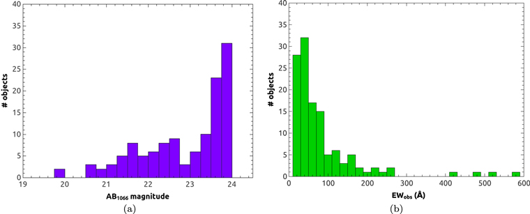
Figure 3. (a) Narrow-band AB magnitudes, and (b) observed equivalent width distributions of the Hα candidates.
Download figure:
Standard image High-resolution image6. Completeness
In order to accurately determine the detection limits of the DAWN survey, it is necessary to estimate the completeness fraction—that is how the number of objects that our selection methods recover compare to the total number of existing objects. This completeness fraction will depend on both the luminosity and EW of the sources.
The approach to calculating the completeness fraction is to create artificial sources and superimpose them on our science image and repeat all the selection procedures explained in Sections 3.3–3.5 in said image. A comparison between the number of sources added, and the number recovered that were not in the selection with only real objects, yields the recovery fraction. These artificial sources are created as extended sources with a two-dimensional Gaussian shape having the same FWHM as compact galaxies in the survey (∼12).
We repeated this process once for each one of our 800 intervals of luminosity and observed EW, in the range of  in steps of 0.1 dex and an EW of 0–200 Å in 10 Å steps. The nominal detection limits of this survey are
  and
and  , so these intervals assure we cover objects both close and far from the detection limits.
In each simulation, we generated 10,000 artificial galaxies, which corresponds to ≈20% of the sources in the science image. For each artificial object, its narrow-band luminosity and EW are selected randomly from the L-EW interval they correspond to. The J-band luminosity is then derived from
where fNB and fJ are the observed flux densities in the narrow-band and J-band filters, respectively, and ΔNB and ΔJ are the corresponding filters' bandwidths.
The artificial source fluxes are then scaled to counts using the appropriate zero points, and randomly scattered over the science images. Finally, the selection rules are applied to the resulting images.
For each simulation, we define a recovery percentage dependent on the number of objects recovered and the number of real and artificial objects in the image:
In the simulations with lowest EW, the number of objects recovered was lower than in the science image with no added sources. Therefore, we assumed that due to an overcrowding of the image not all the real sources are recoverable, and we took Nreal as the lowest number of objects recovered in the whole set of simulations instead of the number of real emission-line sources in the image.
This completeness correction was applied to each individual source in our Hα sample according to its luminosity and equivalent width.
The LF we find from the DAWN survey, after correction for [N ii], extinction, and incompleteness, is plotted in Figure 4. A summary of the completeness fraction as a function of luminosity and equivalent width can be found in Figure 5.
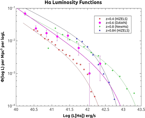
Figure 4. Hα luminosity functions from the DAWN survey at z = 0.62 (pink circles), HiZELS (Sobral et al. 2013) at z = 0.4 (red squares) and z = 0.84 (blue triangles), and NewHα survey (Ly et al. 2011) at z = 0.8 (green diamonds). The plotted luminosity functions are corrected for [N ii], dust, and incompleteness, as described in the text for the DAWN sample, and following the procedures in the original publications for the literature samples. The apparent difference in the bright end of the LF at z ≈ 0.8 from Sobral et al. (2013) and Ly et al. (2011) is dominated by differences in the extinction corrections adopted in the two papers. The DAWN survey points are corrected for extinction using the same procedure as was applied to the Ly et al. (2011) sample.
Download figure:
Standard image High-resolution image
Figure 5. Completeness percentage as a function of Hα luminosity and equivalent width. The minimum equivalent width detected in the DAWN survey, 18 Å, is marked with a red line.
Download figure:
Standard image High-resolution image7. LF Fitting and Star Formation Rate Densities
We construct our LF binning our Hα sample in bins 0.3 dex wide in luminosity. Observed and extinction- and completeness-corrected numbers and number densities as a function of luminosity are listed in Table 4.
Table 3. Luminosity Function Parameters for Different Surveys
| Survey | z | log 
|
log 
|
α |
|---|---|---|---|---|
| DAWN | 0.62 | 42.64 | −3.32 | −1.75 |
| (this work) | ||||
| WySH | 0.16 | 42.0 | −3.05 | −1.36 |
| (Dale et al. 2010) | 0.24 | 41.8 | −2.74 | −1.41 |
| 0.32 | 42.1 | −2.77 | −1.26 | |
| 0.40 | 42.2 | −2.79 | −1.14 | |
| HiZELS | 0.40 | 41.95 | −3.12 | −1.75 |
| (Sobral et al. 2013) | 0.84 | 42.25 | −2.47 | −1.56 |
| 1.47 | 42.56 | −2.61 | −1.62 | |
| 2.23 | 42.87 | −2.78 | −1.59 | |
| NewHα | 0.84 | 43.0 | −3.2 | −1.6 |
| (Ly et al. 2011) | ||||
| Villar et al. (2008) | 0.84 | 42.97 | −2.76 | −1.34 |
| Hayes et al. (2010) | 2.2 | 43.07 | −3.45 | −1.6 |
Download table as: ASCIITypeset image
Our LF is fitted to a Schechter (1976) function defined by the parameters  , L*, and α:
In the log form, this equation translates into
We assume that this function can be accurately used to model the distribution of Hα luminosities. This approach has also been extensively used in the past, which makes it ideal to compare our results to previous work (Villar et al. 2008; Ly et al. 2011; Sobral et al. 2013).
Table 4. Extinction and Completeness-corrected Hα Luminosity Function at z ∼ 0.62
| log(L[Hα]) | Nobserved | Ncorrected | Φ(log L) |
|---|---|---|---|
| 40.25 | 48 | 69 | 6.95 ± 0.83 |
| 40.55 | 16 | 24 | 2.45 ± 0.49 |
| 40.85 | 16 | 17 | 1.74 ± 0.42 |
| 41.15 | 13 | 13 | 1.38 ± 0.37 |
| 41.45 | 14 | 14 | 1.45 ± 0.38 |
| 41.75 | 6 | 6 | 0.61 ± 0.25 |
| 42.05 | 1 | 1 | 0.10 ± 0.10 |
| 42.35 | 2 | 2 | 0.20 ± 0.14 |
Note. Φ(log L) is normalized to  .
.
Download table as: ASCIITypeset image
In order to obtain the confidence range of the best-fitting Schechter parameters, we performed a Monte Carlo simulation to consider the full range of scatter in the extinction-corrected Hα LF. Each point in the binned LF was randomly perturbed 2500 times following a Gaussian distribution, with the variances of the Gaussian drawn according to its error bars. Then, we calculated the best fit to a Schechter function for each of these simulations using a χ2 fit. It is worth noting that most of these fittings were more consistent with a power-law than with a Schechter function, as it can be seen in Figure 6. However, the Schechter function is the best fit to the original data, and is the preferred functional form in the literature because it generally provides a better fit than a pure power-law. The degeneracy between Schechter and power-law forms in the present analysis arises because  for the single DAWN field analyzed herein, so that the absence of objects with
  does not strongly rule out
  . It is not sensible to suppose that our survey would find a region where the functional form of the LF is different from the predominant one at both lower and higher redshifts. Therefore we use a Schechter function for our further analysis, and estimate the uncertainties in the parameters from the Schechter function fits to the simulations.

Figure 6. Best fit Schechter luminosity function parameters for our ∼2500 Monte Carlo simulations. Although a Schechter function provides the best fit to our actual luminosity function data (Figure 4), a pure power-law gives a somewhat better fit to the majority of our simulations. This ambiguity results in some pileup of the simulations near large L∗ and low Φ*. We regard this as likely unphysical, since it is unlikely that our survey would find a region where the functional form of the luminosity function is different from the predominant one at both lower and higher redshifts. Therefore we adopt a Schechter function for our further analysis.
Download figure:
Standard image High-resolution imageThe best-fitting parameters are determined to be  erg s−1,
  Mpc−3, and α = −1.75 ± 0.09. The uncertainties in L* and Φ* are strongly anticorrelated, as seen in Figure 6.
The integrated Hα luminosity density can then be calculated from the Schechter parameters:
The integrated Hα luminosity density can subsequently be converted into an SFR density following Kennicutt (1998): SFR(Hα) = 7.9 × 10−42 L(Hα), where the SFR is given in M⊙ yr−1 and the Hα luminosity is given in erg s−1. We determine that the Hα SFR density is ρSFR = 10−1.32 ± 0.08 M⊙ yr−1 Mpc−3 down to L = 0. If we calculate the SFR density down to our luminosity limit ( ), this result decreases to ρSFR = 10−1.42 ± 0.08 M⊙ yr−1 Mpc−3.
In order to account for the presence of AGNs, we compared our catalog of Hα candidates to the XMM-Newton wide-field survey (Cappelluti et al. 2009) and the Chandra Cosmos Legacy Survey catalogs (Civano et al. 2016), but no matches were found. (While there were DAWN emission-line objects that matched X-ray sources, none of those were identified as Hα emitters.) As no measurement of the X-ray emission of our candidates is available, we follow the approach described in Ly et al. (2011) and correct the value presented above by 11%. Similar approaches have been used in other surveys. For example, Sobral et al. (2013) used a 10% correction up to z ∼ 1. Sobral et al. (2016) published AGN fractions for objects with  , which can be larger at high luminosities. However, all but three objects from our sample have lower luminosities, and the AGN corrections reported by Sobral et al. (2016) at
  are consistent with the 11% we have used. Our 11% AGN correction reduces the total DAWN survey Hα SFR density to ρSFR = 10−1.37 ± 0.08 M⊙ yr−1 Mpc−3 when integrated down to L = 0, and to ρSFR = 10−1.47 ± 0.08 M⊙ yr−1 Mpc−3 down to L = Lmin. We plot the SFR density from DAWN and from other H alpha surveys spanning the redshift range 0 < z < 2.3 in Figure 7.
Madau & Dickinson (2014) provide an experimental fit to the total SFR density as a function of redshift ( ). Following their procedure, we obtain a total star formation density of
  M⊙ yr−1 Mpc−3 at z ∼ 0.62. This result implies that galaxies like those in our sample account for roughly 80% of the total SFR density at z ∼ 0.62.
8. Hα Sizes
We compare our Hα sample with the "COSMOS ACS catalog" (Leauthaud et al. 2007) in order to obtain the sizes (half-light radii) of the emitters in our sample. Out of our 116 objects, 115 are found in said catalog.
We divide our sample in two sub-samples, according to the Hα luminosity of the sources. We have a faint sample containing 79 sources with log(L) ≤ 41.0 and a bright sample containing 36 sources with log(L) > 41.0.
The median half-light radius for the whole sample is 027 (1.85 kpc), while it is 022 (1.5 kpc) for the faint sample and 039 (2.7 kpc) for the bright sample. The interquartile range for the whole sample is 018–038 (1.2–2.6 kpc), while it is 017–030 (1.2–2.1 kpc) for the faint sample and 029–054 (2.0–3.7 kpc) for the bright sample. It can be seen that the dimmer objects also tend to be smaller, showing a correlation between luminosity and size in Hα emitters. The z ≈ 0.62 DAWN sample objects are slightly smaller than the Hα selected samples at z ≈ 0.4 and 0.84 presented for HiZELS survey sources in Stott et al. (2013) and Paulino-Afonso et al. (2017). This could occur if differences in sample selection yield a smaller typical stellar mass for the DAWN sample than for the HiZELS samples. Alternatively, it could result from differences in half-light radius measurement techniques. We are using purely space-based re measurements, while the HiZELS studies incorporate ground-based measurements appropriately corrected for seeing, which could be a significant effect, especially for the small radii observed here. Interestingly, although small, the DAWN Hα selected samples remain larger than either Lyα selected objects at z ≳ 2 (Malhotra et al. 2012) or in "green pea" galaxy samples (i.e., galaxies selected for extremely strong [O iii] emission) at z ≲ 0.3 (Yang et al. 2017).
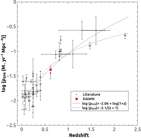
Figure 7. SFR density from Hα surveys. The red square is our measurement, and the black circles are measurements from the literature (a combination of results from Gómez-Guijarro et al. 2016, Ly et al. 2011, Sobral et al. 2013, and literature data compiled in Ly et al. 2011 and Sobral et al. 2013: Gallego et al. 1995; Tresse & Maddox 1998; Yan et al. 1999; Sullivan et al. 2000; Tresse et al. 2002; Fujita et al. 2003; Hippelein et al. 2003; Pérez-González et al. 2003; Brinchmann et al. 2004; Hopkins 2004; Nakamura et al. 2004; Hanish et al. 2006; Hopkins & Beacom 2006; Ly et al. 2007; Geach et al. 2008; Morioka et al. 2008; Shioya et al. 2008; Villar et al. 2008; Westra & Jones 2008; Shim et al. 2009; Sobral et al. 2009; Dale et al. 2010; Westra et al. 2010). The dashed blue line is the fit derived in Dale et al. (2010) for z < 2, while the dashed pink line is the fit derived in Sobral et al. (2013). Our measurement is consistent with both fits. All the points include corrections for dust extinction, but other differences may not be fully accounted for.
Download figure:
Standard image High-resolution imageThe size distribution for the full Hα sample along with that of the bright subsample can be found in Figure 8.

Figure 8. Size distribution for the DAWN Hα sample along with the size distribution of the brighter subset having log(L) > 41.0. Galaxies with lower Hα luminosities are found to have smaller average sizes than those with higher luminosities. (Note, 1 arcsec corresponds to 6.9 kpc at this redshift.)
Download figure:
Standard image High-resolution image
9. Discussion
In Figure 4 we show the extinction and completeness-corrected LF for the DAWN survey, the NewHα survey and the HiZELS survey at z = 0.4 and z = 0.84. The LF parameters for the three surveys can be found in Table 3.
The bright end of the LF agrees with HiZELS (Sobral et al. 2013) at z = 0.84, NewHα (Ly et al. 2011) at z = 0.84, and Villar et al. (2008) also at z = 0.84. The number density of objects obtained from the DAWN survey is consistent with that of all these surveys too.
However, the biggest strength of the DAWN survey is the tight constraint on the slope of the faint end of the LF, α. Our result is consistent with that of previous surveys at similar redshifts, but provides a smaller error bar due to reaching fainter objects. It is worth noting that although the value of α reported in Villar et al. (2008) is shallower, that value was fixed in their calculations due to a lack of faint data.
In Figure 7 we show our measurement for Hα SFR density, along with a compilation of measurements from other surveys that have used that same emission line. This figure shows both statistical uncertainties and cosmic-variance-related uncertainties (calculated following Trenti & Stiavelli 2008) for the DAWN survey measurement. The compilation was originally made by Dale et al. (2010) and reproduced and corrected for mistakes found in the original papers by Ly et al. (2011). We also add results presented in Sobral et al. (2013) and Gómez-Guijarro et al. (2016). The SFR density obtained from the DAWN survey is consistent with those of previous surveys at redshift z < 2 (as are other recent surveys at slightly lower redshift; Drake et al. 2013; Gunawardhana et al. 2013; Stroe & Sobral 2015). The DAWN results refine our understanding with a more precise measurement than prior surveys at 0.5 < z < 0.8.
10. Conclusions
We have presented new measurements of the Hα LF and SFR volume density for emission-line galaxies at z ∼ 0.62. These measurements are based on 1.06 μm narrow-band imaging from the DAWN survey. This survey fills a gap in the redshift coverage for Hα LF studies.
The DAWN survey has a 5σ emission-line flux depth of  and an area coverage of ∼0.22 deg2 in the COSMOS field. We identified 847 narrow-band excess emitters above 5σ, and 116 of them were identified as Hα emission-line galaxies at z ∼ 0.62. This classification is done by comparison with both photometric and spectroscopic redshift catalogs.
We constructed the extinction and completeness-corrected Hα LF. Corrections for dust attenuation and [N ii] contamination were applied. The LF is well described by a Schechter function with  erg s−1,
  Mpc−3,
  erg s−1 Mpc−3, and α = −1.75 ± 0.09. Cosmic variance implies an additional uncertainty of ≈20% in Φ* and in
  . The faint end slope, α, is consistent with but better constrained than earlier works at redshifts 0.4 < z < 0.85.
Integrating the LF to L = 0, we determine a SFR density of log(ρSFR/M⊙ yr−1 Mpc−3) = −1.37 ± 0.08 (random) ± 0.09 (cosmic variance). This luminosity density is consistent with the interpolation of prior measurements at lower and higher redshifts, and provides the most precise z = 0.62 SFRD measurement yet.
We thank NOAO for the generous allocation of observing time for the DAWN survey, and the Kitt Peak staff for their expert support of DAWN observations. We thank Kimberly Emig, Raviteja Nallapu, Emily Neel, Mark Smith, Stephanie Stawinski, Jacob Trahan, Nicholas Valverde, and Trevor Van Engelhoven for their help with DAWN survey observing runs. We thank an anonymous referee for helpful comments that have improved the manuscript. Finally, we thank the US National Science Foundation for its financial support through NSF grant AST-0808165, which supported our custom narrow-band filter purchase, and AST-1518057, which supported our data analysis. We also thank NASA for financial support via WFIRST Preparatory Science Grant NNX15AJ79G, which provided additional support for our scientific analysis.