


Abstract
We apply a friends-of-friends algorithm to the HectoMAP redshift survey and cross-identify associated X-ray emission in the ROSAT All-Sky Survey data (RASS). The resulting flux-limited catalog of X-ray cluster surveys is complete to a limiting flux of ∼3 × 10⁻¹³ erg s−1 cm−2 and includes 15 clusters (7 newly discovered) with redshifts z ≤ 0.4. HectoMAP is a dense survey (∼1200 galaxies deg−2) that provides ∼50 members (median) in each X-ray cluster. We provide redshifts for the 1036 cluster members. Subaru/Hyper Suprime-Cam imaging covers three of the X-ray systems and confirms that they are impressive clusters. The HectoMAP X-ray clusters have an LX–σcl scaling relation similar to that of known massive X-ray clusters. The HectoMAP X-ray cluster sample predicts ∼12,000 ± 3000 detectable X-ray clusters in RASS to the limiting flux, comparable with previous estimates.
Export citation and abstract BibTeX RIS
1. Introduction
Searching for clusters of galaxies is a stepping stone toward understanding galaxy evolution in dense environments (e.g., Dressler 1984; Blanton & Moustakas 2009; Wetzel et al. 2014; Haines et al. 2015), and the formation of large-scale structure (e.g., Bahcall 1988; Postman et al. 1992; Reiprich & Böhringer 2002; Chon et al. 2013), and for evaluating the cosmological parameters (e.g., Voit 2005; Vikhlinin et al. 2009; Allen et al. 2011; Böhringer et al. 2014). A large cluster catalog provides a sample for statistical studies of the formation and evolution of galaxies within dense, massive, gravitationally bound systems. Simultaneously, the number density and mass distribution of the ensemble of galaxy clusters are important probes of cosmological models.
A wide variety of techniques yield cluster catalogs. Initial systematic surveys for clusters identified overdensities of galaxies on the sky (Abell 1958; Zwicky et al. 1968; Abell et al. 1989). Many recent studies use the red sequence that generally characterizes cluster galaxies along with the brightest cluster galaxies (BCGs) to identify clusters (Gladders & Yee 2000; Koester et al. 2007; Hao et al. 2010; Oguri 2014; Rykoff et al. 2014; Oguri et al. 2017). Often, the redshifts for these large photometric samples are photometric (Wen et al. 2009, 2012; Szabo et al. 2011; Durret et al. 2015). These catalogs contain a large fraction of real systems, but they cannot discriminate completely against line-of-sight superpositions. Cluster identification based on spectroscopic redshifts resolves the contamination issue, but the density of a spectroscopic survey can be a limiting factor in evaluating the completeness and purity of the catalog.
Large galaxy cluster catalogs are also based on X-ray identification. The ROSAT All-Sky Survey (RASS) data have been especially important (Ebeling et al. 1998, 2010; Böhringer et al. 2000, 2004, 2013, 2017). The Sunyaev–Zel'dovich (SZ) effect (Sunyaev & Zeldovich 1972) is a more recent but equally powerful tool for identifying clusters (Vanderlinde et al. 2010; Marriage et al. 2011; Bleem et al. 2015; Planck Collaboration et al. 2015, 2016). For verification of both the X-ray and SZ candidates, optical counterparts identified from imaging and/or spectroscopy are critical. Optical follow-up observations for the Northern ROSAT All sky survey (NORAS) found optical clusters associated with 76% of the X-ray extended sources (Böhringer et al. 2000). Similarly, Bleem et al. (2015) showed that 76% of the South Pole Telescope (SPT)-SZ clusters with 4.5σ detection are confirmed by optical and/or near-infrared imaging.
Cluster catalogs are also constructed from complete spectroscopic surveys (e.g., Geller & Huchra 1983; Mahdavi et al. 2000; Finoguenov et al. 2009; Robotham et al. 2011; Tempel et al. 2016). Mahdavi et al. (2000) identified galaxy groups based on a complete spectroscopic survey. After identification of the spectroscopic candidates, they searched RASS for these objects. This cross-identification identified the most reliable systems. More recently, Starikova et al. (2014) followed a similar procedure where clusters were first identified with a combination of spectroscopic and weak lensing observations and followed with X-ray observations. Combining a spectroscopic survey with other cluster identification techniques is a powerful approach because it provides direct cluster membership with little line-of-sight contamination. Furthermore the spectroscopic redshifts enable an estimate of the dynamical mass of the systems for direct comparison with X-ray, SZ, and weak lensing measurements.
Here, we follow an approach similar to the one pioneered by Mahdavi et al. (2000). We explore a much deeper redshift survey to a limiting r = 21.3. We use the HectoMAP (Geller et al. 2011; Geller & Hwang 2015) redshift survey to identify massive candidate systems based on a friends-of-friends (FoF) algorithm. We then use RASS to search for X-ray emission associated with the clusters in the HectoMAP region and to test whether the X-ray emission is consistent with emission from a hot thermal intracluster plasma. We also check the HectoMAP cluster catalog against previously published X-ray cluster candidates. We test our approach by applying an identical technique to the Smithsonian Hectospec Lensing Survey (SHELS) redshift survey (Geller et al. 2010, 2012, 2014) explored by Starikova et al. (2014).
HectoMAP is a dense redshift survey complete to r = 21.3 and with a median redshift of z ∼ 0.39. The red-selected HectoMAP survey is 95% complete in the selected color range, (g − r)fiber,0 > 1.0 and (r − i)fiber,0 > 0.5. Using this survey, Hwang et al. (2016) examined large-scale structures and voids in comparison with the result from the Horizon Run 4 N-body simulation (Kim et al. 2015). The observed richness and size distributions of both overdense and underdense structures agreed well with the simulations.
The catalog of HectoMAP galaxy clusters described here depends on cross-identification with the X-rays. We apply the FoF to the complete color-selected galaxy catalog. We refine the FoF cluster membership by applying the caustic technique to all of the data in the HectoMAP region. In the catalog, we identify 15 robust clusters with a median of ∼50 spectroscopically identified members. Seven of these clusters have not been previously identified. We examine their physical properties, including X-ray luminosities and velocity dispersions. These detections suggest that even to the limit of RASS there are more than ∼12,000 detectable massive X-ray clusters to a flux limit of ∼3–5 × 10⁻¹³ erg s−1 cm−2 in the 0.1–2.4 keV energy band compatible with the estimate by Schuecker et al. (2004). These clusters are typically at redshifts of less than 0.4. This sample hiding in the existing RASS data is larger than the SPT samples (Bleem et al. 2015).
We describe the spectroscopic data from HectoMAP and X-ray data from RASS in Section 2. Section 3 explains the cross-identification techniques, including a description of the cluster finding methods. The cluster catalog is in Section 4. We also include redshifts of the 1036 cluster members. We discuss the results, including the physical properties of the clusters, in Section 5, and summarize in Section 6. We adopt the standard ΛCDM cosmology of H0 = 70 km s−1 Mpc−1, Ωm = 0.3, and ΩΛ = 0.7 throughout the paper.
2. Data
Selecting clusters from a redshift survey is only possible when the sampling density is sufficiently high (e.g., CNOC survey, Yee et al. 1996). HectoMAP has a density of ∼2000 galaxies deg−2 to a limit rpetro,0 = 21.3; the median depth of the redshift survey is 0.39. Our approach here is to identify cluster candidates by applying an FoF to the redshift survey and then using the resultant catalog as a finding list for extended X-ray sources in RASS.
We first describe the salient features of HectoMAP (Section 2.1). Then, we review RASS detection limits relevant for testing the HectoMAP candidate clusters against the X-ray data (Section 2.2).
2.1. HectoMAP: A Dense Spectroscopic Survey
HectoMAP is a dense redshift survey of red galaxies covering 52.97 deg2 of the sky with 200 < R.A. (degree) < 250 and 42.5 < decl. (degree) < 44.0 (Geller et al. 2011; Geller & Hwang 2015; Hwang et al. 2016). We select HectoMAP galaxies from the Sloan Digital Sky Survey (SDSS) Data Release 9 (DR9) (Ahn et al. 2012). We select red galaxies with (g − r)fiber,0 > 1.0, (r − i)fiber,0 > 0.5 as redshift survey targets. The color selection removes objects with z ≲ 0.2 where the SDSS spectroscopic survey has reasonable coverage. The targets have rpetro,0 < 21.3 and rfiber,0 < 22.0. We fill fibers that we cannot allocate to the main HectoMAP red targets with objects bluer or fainter than the target limits. We exclude rfiber,0 > 22.0 objects because their low surface brightness makes the acquisition of a redshift difficult in the standard HectoMAP exposure time.
From 2009 to 2016, we conducted a redshift survey with the 300-fiber spectrograph Hectospec mounted on the Multiple Mirror 6.5 m telescope (MMT; Fabricant et al. 1998, 2005). The fiber-fed spectrograph Hectospec typically obtains spectra for ∼250 targets within a ∼1 deg2 field of view in a single observation. The 270 line mm−1 grating yields a wavelength range of 3700–9150 Å with a resolution of ∼6.2 Å. The exposure time for each field is 0.75–1.5 hr and each exposure is comprised of three subexposures for cosmic-ray removal. To guarantee uniform sampling even in the densest regions, we revisit each HectoMAP position ∼7 times. The completeness map (Figure 1) shows the resulting uniformity of the survey. The only residual non-uniformity occurs toward the edges of the field.
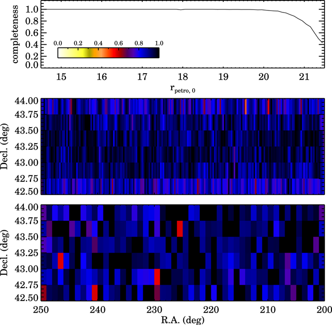
Figure 1. (Top) The differential spectroscopic completeness for HectoMAP as a function of r-band magnitude. (Middle) Two-dimensional completeness map (200 × 6 pixels) of HectoMAP for the galaxies with rpetro,0 ≤ 21.3, (g − r)fiber,0 > 1.0, and (r − i)fiber,0 > 0.5. (Bottom) Same as the middle panel, but for SDSS galaxies with rpetro,0 ≤ 17.77 with larger pixels (25 × 6 pixels).
Download figure:
Standard image High-resolution imageWe also compile previously measured redshifts in the HectoMAP region from SDSS DR14 (Abolfathi et al. 2017) and from the NASA Extragalactic Database (NED). There are 2143 redshifts from SDSS and 161 redshifts from the literature (NED) within the HectoMAP red selection. The typical uncertainties in the redshifts from SDSS and NED are 28 km s−1 and 60 km s−1, respectively. There are no significant zero-point offsets between the SDSS and Hectospec redshifts (Geller et al. 2014).
We reduce the Hectospec spectra using the HSRED v2.0 package originally developed by Richard Cool and substantially revised by the SAO Telescope Data Center (TDC) staff.8 The TDC has tested this reduction against the original HSRED and IRAF SPECROAD packages.9 We derive redshifts using RVSAO (Kurtz & Mink 1998), a cross-correlation code. The set of spectral templates is identical to the set used for earlier reductions of Hectospec data. We visually inspect each spectrum and classify redshifts into three groups: "Q" for high-quality spectra, "?" for ambiguous fits, and "X" for poor fits. We use only "Q" spectra. There are 58211 redshifts for red galaxies satisfying the HectoMAP magnitude and color selection. The typical redshift uncertainty normalized by (1 + z) is ∼32 km s−1.
Figure 1 shows the spectroscopic completeness of HectoMAP to rpetro,0 = 21.3. Hwang et al. (2016) displayed a similar plot for the bright (rpetro,0 < 20.5) portion of HectoMAP, which was 89% complete to this limit at that time. The survey is now 98% complete to rpetro,0 = 20.5.
The upper panel of Figure 1 is the current spectroscopic completeness for red galaxies with (g − r)fiber,0 > 1.0 and (r − i)fiber,0 > 0.5 as a function of apparent magnitude. The integral completeness of the survey to rpetro,0 = 21.3 for the HectoMAP selection is ∼89%. The middle panel shows the two-dimensional completeness map for HectoMAP red galaxies. The survey completeness is fairly homogeneous over the entire field. There are a few streaks of low completeness around the edges of the survey, but even in these regions the completeness exceeds ∼70%. We show a similar two-dimensional completeness map for SDSS Main Sample galaxies plus HectoMAP red galaxies with rpetro,0 < 17.77 in the lower panel. Only ∼10% of the objects satisfy the HectoMAP selection. We note that the SDSS sample is less uniform than the HectoMAP sampling. The SDSS spectroscopic survey is patchy near bright stars or the high-density regions due to the fiber collision.
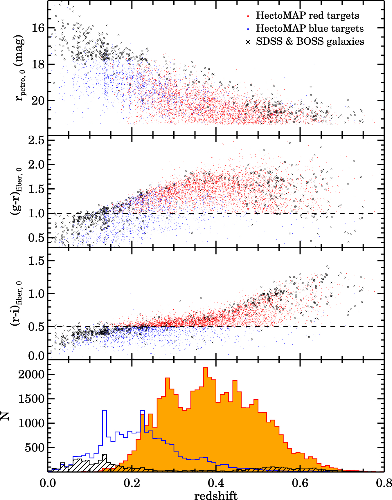
Figure 2 shows the color selection for HectoMAP. For comparison, we plot SDSS galaxies and blue galaxies from HectoMAP. The color selection we adopt effectively selects galaxies with z ≳ 0.2.

Figure 2. (Top) r-band magnitudes as a function of redshift for HectoMAP red galaxies (red), HectoMAP blue galaxies (blue), and HectoMAP galaxies with SDSS spectra (black). (Middle) Same as the top panel, but for (g − r)fiber,0 and (r − i)fiber,0 colors. The dashed lines display the HectoMAP color cuts. (Bottom) Redshift distribution of HectoMAP red galaxies (red filled histogram), the blue galaxies (blue open histogram), and SDSS galaxies (black hatched histogram).
Download figure:
Standard image High-resolution imageWe use the red complete sample as the basis for FoF cluster identification at z > 0.2. At lower redshifts, the r − i selection reduces the sampling density substantially (Figure 2). Thus, in this range we use the SDSS Main Sample supplemented with the red HectoMAP galaxies.
After cross-identifying the FoF candidates with extended X-ray emission in RASS we refine the cluster membership by applying the caustic technique (Diaferio & Geller 1997; Diaferio 1999; Serra & Diaferio 2013) to all galaxies with redshifts in each cluster region. There are 26317 additional redshifts for objects bluer than the HectoMAP cuts. These objects include the SDSS Main Galaxy sample, BOSS galaxies, and bluer galaxies used to fill unused fibers in the Hectospec survey. This caustic analysis increases the typical cluster membership by a factor of ∼1.5 compared to the FoF membership and enables more robust estimates of the cluster velocity dispersion and scale.
2.2. Search for X-Ray Emission in RASS
For all the clusters found by the FoF algorithm in the HectoMAP survey, we searched for X-ray emission in RASS (Truemper 1993). To date, RASS constitutes the only all-sky X-ray survey conducted with an imaging X-ray telescope. The typical flux limit for a detection of at least ∼2.5σ is ∼3–5 × 10⁻¹³ erg s−1 cm−2 in the 0.1–2.4 keV energy band. Detections of this low significance are only justified because we search for emission at predefined positions. The source detection applied for the public RASS source catalog (Voges et al. 1999) had a much higher significance threshold. The typical sky exposure in RASS is of the order of 400 s. For our purposes, the survey is rather shallow, and we expect a detection only for the most prominent systems.
In total, we searched for X-ray emission at the position of 166 FoF clusters in RASS, allowing in the first pass a coincidence radius up to 7 arcmin. We found 15 systems that showed significant X-ray emission. These systems have more than 30 FoF members. The source detection and characterization follow the techniques used for the construction of the REFLEX II and NORAS II cluster surveys (Chon & Böhringer 2012; Böhringer et al. 2013, 2017). In the NORAS and REFLEX surveys we ran our detailed source analysis at positions of a low-threshold RASS X-ray source catalog (Voges et al. 1999). Here, we apply the same technique at the sky positions of the HectoMAP clusters. It uses the ROSAT PSPC detector energy channels 52–201, which roughly correspond to the energy band 0.5–2 keV, because in this energy band the signal-to-noise ratio is maximized. At lower energies a large part of the X-ray emission is absorbed by the interstellar medium of our Galaxy and the galactic X-ray background is high. Above 2 keV, there is a sharp cutoff in the reflectivity of the ROSAT mirror.
To measure the X-ray fluxes and to characterize the X-ray sources, we apply the growth curve analysis method described in Böhringer et al. (2000). In brief, the background-subtracted cumulative source count rate is determined with an increasing aperture, and the fiducial source radius is identified with the location where the count rate reaches a stable plateau. The X-ray source position is determined from the mean sky position of the source photons detected in an aperture of three arcmin radius. The offsets of the X-ray positions from the HectoMAP cluster positions are in Table 1.
Table 1. HectoMAP X-Ray Clusters
| ID | known ID | R.A.Caustic | Decl.Caustic | z | Nmem | R.A.X-ray | Decl.X-ray | roffseta | fXb | LXc |
|---|---|---|---|---|---|---|---|---|---|---|
| (arcmin) | 10−13 erg cm−2 s−1 | (1044 erg s−1) | ||||||||
| HMxcl162726.7+424052 | RXC J1627.3+4240 | 16:27:26.7 | +42:40:52 | 0.032 | 33 | 16:27:25.0 | 42:40:24 | 0.369 | 27.50 ± 0.28 | 0.06 ± 0.01 |
| HMxcl141341.6+433925 | A1885 | 14:13:41.6 | +43:39:25 | 0.089 | 40 | 14:13:38.7 | 43:40:15 | 1.797 | 34.02 ± 1.36 | 0.66 ± 0.26 |
| HMxcl162134.3+424558 | A2183 | 16:21:34.3 | +42:45:58 | 0.135 | 51 | 16:21:28.0 | 42:45:03 | 0.643 | 19.97 ± 0.39 | 0.87 ± 0.17 |
| HMxcl151550.0+434556 | MCXC 1515.5+4346 | 15:15:50.0 | +43:45:56 | 0.137 | 18 | 15:15:33.0 | 43:46:35 | 0.417 | 8.08 ± 0.40 | 0.40 ± 0.20 |
| HMxcl162632.8+424039 | A2192, WHL J162642.5+424012 | 16:26:32.8 | +42:40:39 | 0.187 | 110 | 16:26:41.1 | 42:40:13 | 0.263 | 1.16 ± 0.06 | 0.15 ± 0.07 |
| HMxcl142837.5+433852 | ... | 14:28:37.5 | +43:38:52 | 0.213 | 30 | 14:28:39.3 | 43:40:14 | 1.368 | 9.79 ± 0.23 | 1.29 ± 0.31 |
| HMxcl150730.7+424424 | WHL J150723.2+424402 | 15:07:30.7 | +42:44:24 | 0.218 | 108 | 15:07:31.7 | 42:44:39 | 1.689 | 13.42 ± 0.43 | 1.58 ± 0.51 |
| HMxcl163445.9+424641 | ... | 16:34:45.9 | +42:46:41 | 0.224 | 218 | 16:35:16.0 | 43:08:23 | 1.687 | 3.90 ± 0.25 | 0.53 ± 0.34 |
| HMxcl150859.8+425011 | ... | 15:08:59.8 | +42:50:11 | 0.241 | 28 | 15:09:01.3 | 42:49:58 | 0.658 | 2.17 ± 0.16 | 0.40 ± 0.29 |
| HMxcl153606.7+432527 | ... | 15:36:06.7 | +43:25:27 | 0.255 | 31 | 15:36:02.6 | 43:26:40 | 0.994 | 17.75 ± 0.26 | 3.17 ± 0.46 |
| HMxcl143543.4+433828 | ... | 14:35:43.4 | +43:38:28 | 0.267 | 57 | 14:35:41.7 | 43:36:43 | 0.907 | 10.82 ± 0.38 | 1.97 ± 0.69 |
| HMxcl163352.9+430529 | WHL J163355.8+430528 | 16:33:52.9 | +43:05:29 | 0.271 | 54 | 16:33:48.9 | 43:04:13 | 1.762 | 4.07 ± 0.12 | 0.91 ± 0.26 |
| HMxcl141109.9+434145 | WHL J141115.4+434123 | 14:11:09.9 | +43:41:45 | 0.299 | 123 | 14:11:12.2 | 43:41:43 | 0.931 | 5.64 ± 0.16 | 1.44 ± 0.40 |
| HMxcl145913.1+425808 | WHL J145912.8+425758 | 14:59:13.1 | +42:58:08 | 0.371 | 39 | 14:59:08.2 | 42:57:50 | 2.239 | 2.96 ± 0.10 | 1.66 ± 0.55 |
| HMxcl132730.5+430433 | ... | 13:27:30.5 | +43:04:33 | 0.372 | 99 | 13:27:28.5 | 43:06:03 | 1.038 | 5.82 ± 0.35 | 2.26 ± 1.35 |
Notes.
aThe distance of the center of X-ray emission from the BCGs. bX-ray flux we measure from ROSAT in units of 10−13 erg cm−2 s−1. The flux is obtained from the plateau of the growth curve analysis method within the rest-frame energy band 0.5–2.0 keV. cX-ray luminosity we measure from ROSAT in units of 1044 erg s−1. The luminosity is corrected to give the values within an aperture of R500.Download table as: ASCIITypeset image
In some cases, nearby X-ray sources have to be deblended interactively to determine a proper source count rate.10 The conversion from count rate to flux is obtained by folding X-ray spectra of hot thermal plasma through the instrument response function of the ROSAT instruments.11 The parameters used for the spectrum calculations are the plasma temperature obtained from the X-ray luminosity-temperature relation (Böhringer et al. 2012), a metal abundance of 0.3 solar, the known cluster redshift, and the interstellar hydrogen column density taken from the 21 cm sky maps of Dickey & Lockman (1990). The luminosities are determined for the rest-frame 0.1–2.4 keV energy band.
In addition to the flux and the luminosity, we determine two further quantities for each source: the probability that the source is extended beyond the point-spread function of the ROSAT instruments and the spectral hardness ratio (e.g., Böhringer et al. 2013). The probability of having extended source emission is evaluated by means of a Kolmogorov-Smirnov test. A probability threshold of less than 1% consistency with a point source is taken as a significant detection of source extent. The hardness ratio of the sources is determined by means of the formula HR = (H − S)/(H + S), where H is the flux in the 0.5–2 keV band and S is the flux at 0.1–0.4 keV. The observed hardness ratio is compared to the one expected for thermal emission from a hot intracluster plasma, enabling the identification of X-ray emission of possible other contaminating X-ray sources contributing to the cluster X-ray flux. These extra source characterization parameters are a great help in strengthening the interpretation of the observed X-ray emission as originating in the cluster's intracluster medium.
3. Cluster Identification
3.1. The FoF Algorithm
We apply a FoF algorithm to identify candidate galaxy clusters in HectoMAP. The FoF algorithm recursively links galaxies within given linking lengths and bundles them into candidate galaxy systems. The FoF algorithm is widely applied because it identifies a unique set of group and cluster candidates in a sample regardless of the geometry of clusters (Berlind et al. 2006). Based on the FoF algorithm, many group and cluster catalogs have been constructed from a wide variety of spectroscopic surveys (Huchra & Geller 1982; Geller & Huchra 1983; Barton et al. 1996; Ramella et al. 1997, 1999; Berlind et al. 2006; Tago et al. 2010; Robotham et al. 2011; Tempel et al. 2012, 2014, 2016; Sohn et al. 2016).
We adopt a standard FoF algorithm that connects neighboring galaxies with separate spatial and radial velocity linking lengths (Huchra & Geller 1982; Geller & Huchra 1983). This application identifies friends of a galaxy if the transverse (ΔDij) and radial (ΔVij) separations are smaller than the selected fiducial linking lengths. Here, the separations between two galaxies (i and j) are

and

where θij is an angular separation between two galaxies and Dc is the comoving distance at the redshift of galaxy.
The choice of linking length is a critical issue. If the linking lengths are too tight, only compact systems are identified and looser galaxy systems are broken into smaller fragments. In contrast, the algorithm links physically distinct systems or even unrelated segments of the large-scale structure into a single cluster if the linking lengths are too generous. Diaferio et al. (1999) also showed that the properties of the candidate clusters, including the number of members, size, and velocity dispersion, vary depending on the linking length.
Previous studies that identified clusters based on a FoF algorithm often chose linking lengths related to the number density of galaxies ( ) at each redshift. In other words, the FoF identified local overdensities as candidate systems. Here, we follow this approach for HectoMAP.
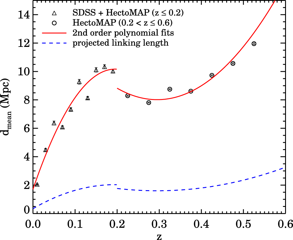
To apply the FoF algorithm to HectoMAP, we first compute the mean separation of galaxies in the complete red-selected sample as a function of redshift. Figure 3 shows the mean separation ( ) as a function of redshift. For galaxies at z ≤ 0.2, we count the number of SDSS galaxies and HectoMAP red galaxies in redshift bins Δz = 0.02 and divide by the comoving volume. In this redshift range, most redshifts of galaxies in the HectoMAP region are from SDSS. For galaxies at 0.2 < z ≤ 0.6, we calculate the mean separation of the HectoMAP red galaxies in redshift bins Δz = 0.05.
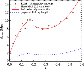
Figure 3. Mean separation (dmean) of the spectroscopically sampled red galaxies in HectoMAP (black circles). The red solid line shows the second-order polynomial fit for 0.2 < z ≤ 0.6. The blue dashed line is the projected linking length (0.2 × dmean) we apply for identifying clusters in the higher-redshift subsample as a function of redshift. The radial linking length is the same as dmean.
Download figure:
Standard image High-resolution imageAt both z ≤ 0.2 and 0.2 < z ≤ 0.6, the mean separation of galaxies increases smoothly as a function of redshift. The solid red curves show second-order polynomial fits to the mean separations. We then apply variable linking lengths according to these fits to the effective survey number densities for each redshift range.
The variable linking lengths related to the survey number density are

and

where b⊥ and  are scaling factors for the transverse and radial linking lengths. This application identifies clusters as overdensities at different redshifts. The b⊥ determines the system overdensity according to

(Huchra & Geller 1982; Geller & Huchra 1983; Diaferio et al. 1999; Duarte & Mamon 2014).
Although many studies have applied the FoF algorithm with variable linking lengths, there is no strong agreement on the choice of linking lengths (Duarte & Mamon 2014). Previous studies employed b⊥ ranging from 0.06 to 0.23 and a fixed  ratio ∼5–10. Several studies tested the choice of linking lengths by measuring the group completeness and reliability in comparison with mock group catalogs derived from N-body simulations (Frederic 1995; Merchán & Zandivarez 2002; Eke et al. 2004; Berlind et al. 2006; Robotham et al. 2011). However, Berlind et al. (2006) argued that no combination of b⊥ and
  identifies clusters that simultaneously recover the halo multiplicity function and the distribution of projected size and velocity dispersion for these systems.
Here, we use linking lengths b⊥ = 0.2 and  (
( ). Our b⊥ identifies systems that have δn/n ∼ 29. The limiting overdensity is fixed throughout the redshift range. The set of linking lengths is somewhat generous compared to previous studies.
We use the FoF algorithm only as a basis for an X-ray-detected cluster catalog in the HectoMAP region. We would rather include false candidates than exclude real ones. We next show that this approach recovers the relevant set of X-ray clusters in a separate densely surveyed region with essentially full X-ray coverage (Starikova et al. 2014).
We test the FoF on the SHELS survey (Geller et al. 2010, 2012, 2014, 2016), a dense complete redshift survey with no color selection and covering two well-separated 4 deg2 fields (F1 and F2) of the Deep Lens Survey (DLS, Wittman et al. 2002). We use the F2 survey alone for this investigation because it has essentially complete X-ray coverage of all of the possible massive systems in the appropriate redshift range. The F2 survey is ∼95% complete to R ≤ 20.6 with a number density of ∼3200 galaxies deg−2.
In total, there are 26 X-ray-extended sources detected based on Chandra and XMM X-ray data (Starikova et al. 2014); 18 of these X-ray sources are in the redshift range 0.2 < z ≤ 0.6 of interest for testing our approach to HectoMAP X-ray clusters. Here, we select 12 X-ray sources within 0.2 < z ≤ 0.5 for testing our cluster identification procedure because the F2 magnitude limit R ≤ 20.6 is ∼0.4 mag brighter than the HectoMAP limit. The brighter F2 limit precludes FoF cluster detection at z ≳ 0.5. The X-ray flux limit for the 12 X-ray-extended sources with z < 0.5 is 4.3 × 10⁻¹⁵ erg cm−2 s−1 within 0.5–2.0 keV energy band. This X-ray flux limit is nearly two orders of magnitude fainter than the one we reach for the HectoMAP systems.
Starikova et al. (2014) showed that 10 of these sources have optical counterparts identified as clusters in the SHELS spectroscopic survey (Geller et al. 2010) or in the DLS weak lensing analysis (Wittman et al. 2006). Here, we examine the number of F2 X-ray extended sources recovered by the FoF algorithm with the HectoMAP choice of linking lengths.
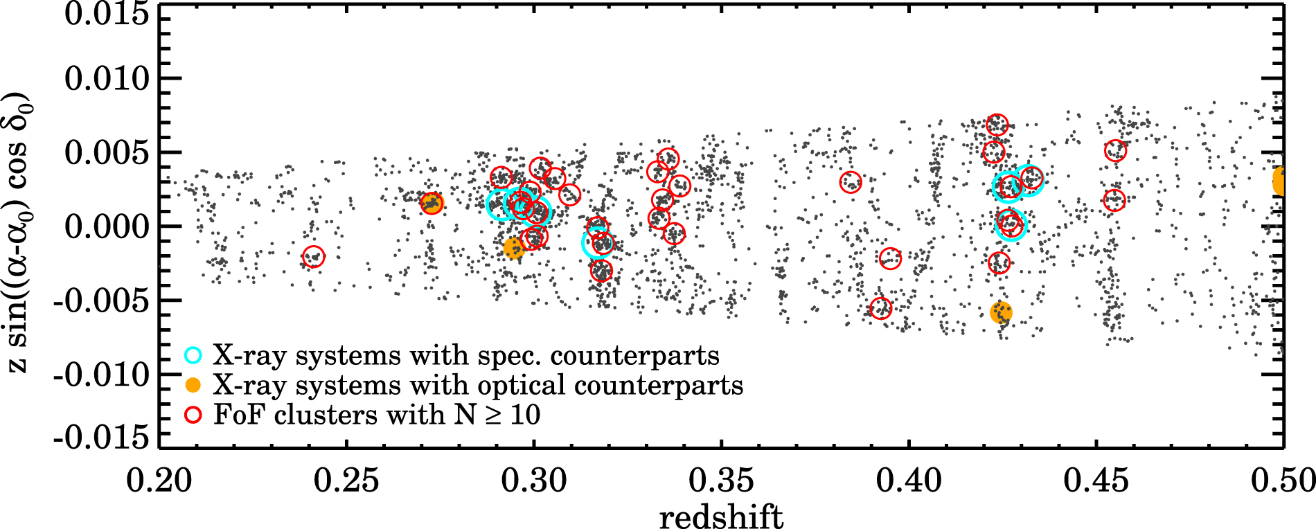
Figure 4 shows the cone diagram of the subset of F2 galaxies selected according to the HectoMAP red galaxy prescription within 0.2 < z ≤ 0.5. In Figure 4, the cyan circles display the locations of seven X-ray-extended sources with spectroscopically identified counterparts from Geller et al. (2010). We also show the X-ray extended sources (yellow circles in Figure 4) matched with weak lensing peaks (Wittman et al. 2006) or with optical concentrations on the sky in the DLS images (Starikova et al. 2014). The redshifts of these X-ray sources with photometrically identified counterparts may not be accurate because they are based on photometric redshifts.

Figure 4. Cone diagram for the SHELS F2 survey subsample with R ≤ 20.6, (g − r)fiber,0 > 1.0, (r − i)fiber,0 > 0.5 projected in the R.A. direction. The cyan and yellow circles indicate extended X-ray sources in F2 with spectroscopic counterparts (Geller et al. 2010) and photometric counterparts (Wittman et al. 2006; Starikova et al. 2014), respectively. The red circles display FoF cluster candidates containing more than 10 members. Every extended X-ray source with a spectroscopic counterpart is recovered by the FoF algorithm.
Download figure:
Standard image High-resolution imageIn summary, the FoF algorithm identifies six systems with N ≥ 10 that match extended X-ray sources in the redshift range 0.2 < z ≤ 0.5. All X-ray sources with spectroscopically identified counterparts have FoF counterparts; one large FoF system at z = 0.29 includes two of these X-ray extended sources. Starikova et al. (2014) showed that with detailed modeling the FoF system resolves in a way that corresponds to the two extended X-ray sources. These massive systems in A781 complex (z = 0.298) are very close together on the sky and they are difficult to separate in the spectroscopic data without a more detailed analysis (Geller et al. 2010). Among the four X-ray extended sources lacking FoF counterparts, all were identified only as apparent photometrically identified overdensities in Starikova et al. (2014). One of these sources does match an FoF system with N = 5. We find no FoF systems associated with the other three X-ray sources, either because their redshifts are incorrect, or because they are contaminated by unresolved X-ray point sources. The performance of the FoF approach over the range accessed by the redshift survey supports the application of this approach to the detection of X-ray clusters to a brighter X-ray flux limit in the HectoMAP data.
To identify cluster candidates over the full redshift range of HectoMAP, we apply the FoF algorithm to separate samples for z ≤ 0.2 and for 0.2 < z ≤ 0.6. For z < 0.2, we select the combined SDSS Main Sample galaxies and HectoMAP red galaxies as the basic galaxy sample. For 0.2 < z ≤ 0.6, we only use the HectoMAP red galaxies to identify cluster candidates. We follow this approach because the HectoMAP r − i cut removes most galaxies at z ≲ 0.2, thus compromising cluster identification in this range based on HectoMAP galaxies alone.
The FoF algorithm detects 166 candidate systems, each consisting of at least 10 galaxies. Figure 5 shows the redshift distribution of these candidate systems. In Figure 5, we mark the 15 clusters with associated extended X-ray emission. The approximate flux limit for X-ray-detected systems is ∼3 × 10⁻¹³ erg cm−2 s−1. None of the HectoMAP clusters at z > 0.4 are detected in RASS. Detecting them would require high X-ray luminosity (cluster mass). For example, the fluxes of the three z > 0.4 X-ray clusters in F2 field are 1.6, 1.9, 0.2 × 10⁻¹³ erg s−1 cm−2, below our X-ray detection limit.
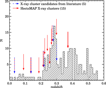
Figure 5. Redshift distribution of FoF cluster candidates in HectoMAP. The red and blue arrows mark the redshifts of the HectoMAP X-ray clusters and clusters from the literature, respectively.
Download figure:
Standard image High-resolution image3.2. X-Ray Counterpart of FoF Clusters
Of the clusters detected with the FoF algorithm, 15 systems show significant X-ray emission in RASS. The number of net source photons found ranges from 6 to 57 (with the exception of HMxcl141341.4+433925 with 128 source photons, which is discussed below). The RASS sky has a low background and the detections are significant even with a low number of photons, but the characterization of the sources becomes difficult with few photons. Thus, we are not expecting to find that all the cluster sources to have significantly extended X-ray emission. Indeed, five of the clusters do not fulfill our criterion for source extent. These clusters are all detected with less than 30 photons. Therefore, the failure to establish a source extent is not an argument against their cluster nature. All the sources with more than 30 photons show a clear extent.
All clusters show a spectral hardness ratio consistent with that expected from thermal emission of a hot intracluster plasma. The only exception is the cluster HMxcl141341.6+433925, which shows spectral parameters indicating that the X-ray emission is too soft for intracluster plasma emission. There is no signature of a positional difference of a softer and harder X-ray source. Therefore, the most likely explanation for the softness of the X-ray source is that there is the contribution of an active galactic nucleus (AGN) in the BCG located exactly at the X-ray center and X-ray maximum of the X-ray source. Since the X-ray source is clearly extended, not all the emission can come from the AGN and we can put an upper limit that no more than 50% of the X-ray flux can come from the AGN. Fitting a point source to the source profile of HMxcl141341.6+433925, we obtain a maximum flux for the point source of 0.27 × 10⁻¹² erg s−1 cm−2, ∼49% of the total source flux.
3.3. Caustic Method and Cluster Membership
We use the caustic technique to refine the definition of the X-ray clusters and to determine the cluster membership. We run the FoF algorithm on the complete red galaxy sample alone. However, the Hectospec survey contains many objects outside the color cuts that are useful for calculating the properties of the clusters. We incorporate these objects in the caustic analysis.
The caustic technique is a powerful tool for identifying cluster members (Diaferio & Geller 1997; Diaferio 1999; Serra & Diaferio 2013). This non-parametric technique determines the boundaries of clusters (caustics), which delimits the location of the cluster members. Serra & Diaferio (2013) test the membership determination based on the caustic technique, with mock catalogs containing ∼1000 galaxies within a field of view of 12 Mpc h−1 on a side at the cluster location. Their simulations show that ∼92% of cluster members are recovered for clusters containing at least ∼50 members within R200; the contamination from interlopers is ∼3%. Because the X-ray detected HectoMAP clusters have a few tens of members, we expect the caustic technique to identify cluster members with a similar success rate.
The caustic technique is also effective for disentangling structures along the line of sight; these structures may be falsely linked by the generous radial linking length we use. For example, Rines et al. (2013) distinguished the pair of clusters A750 and MS0906+11, based on the caustic technique. The radial separation between two clusters is ∼3250 km s−1. The caustics for the two clusters clearly segregate members of the superimposed clusters (Figure 9 of Rines et al. 2013).
We calculate caustics based on galaxies with redshifts within the 30 arcmin of the cluster centers determined by the FoF algorithm. In determining cluster boundaries, the caustic technique also revises the cluster center and the mean redshift. Hereafter, we use the cluster centers and redshifts from the caustic technique.
Figure 6 displays the rest-frame clustercentric velocity as a function of projected clustercentric distance, the  diagram, for the galaxies in the 15 HectoMAP FoF clusters with X-ray counterparts. The
  diagrams show clear concentrations around the center of each cluster. The solid lines in each panel mark the boundaries of the clusters identified by the caustic technique. The galaxies within these caustic patterns are cluster members.
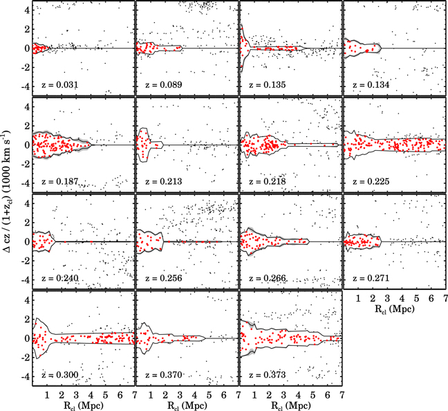
Figure 6. Rest-frame clustercentric radial velocities vs. projected clustercentric distance ( diagrams) for HectoMAP X-ray clusters sorted by redshifts. Black points are galaxies along the line of sight and red points are clusters members within the caustics. The black solid lines show the caustics and the gray shaded regions indicate the uncertainty in the caustic estimate.
Download figure:
Standard image High-resolution imageThe caustic technique also provides the cluster mass profile (Diaferio & Geller 1997; Diaferio 1999; Serra et al. 2011). Based on this mass profile, we compute the characteristic cluster mass and size, i.e., M200 and R200. The mass of HectoMAP X-ray clusters ranges from 2 × 10¹³ M⊙ to 4 × 10¹⁴ M⊙, comparable with the CIRS (Rines & Diaferio 2006) and HeCS (Rines et al. 2013) samples. We estimate the velocity dispersion of each cluster using the method given in Danese et al. (1980). Hereafter, σcl denotes the rest-frame line-of-sight velocity dispersion for cluster members within R200.
4. A Catalog of HectoMAP FoF Clusters with X-Ray Emission
We identify 15 robust clusters in HectoMAP based on the FoF method combined with the identification of X-ray emission in RASS. Hereafter, we refer to these HectoMAP FoF clusters with X-ray counterparts as HectoMAP X-ray clusters. We identify the BCGs among the spectroscopically determined cluster members. Out of 15 systems, 6 contain a galaxy brighter than the BCGs within Rcl < 3' and without a redshift. These objects are most likely foreground blue objects excluded by the HectoMAP selection. The SDSS photometric redshift estimate for these objects suggests that they are all foreground objects. The projected distances between these galaxies and the cluster center is also larger than normal for a BCG. The offset between X-ray emission for the systems and the BCGs of the clusters is consistent with the ROSAT PSF (∼2', Boese 2000). For one system, HMxcl145913.1+425808, the offset between the X-ray emission and the BCG is slightly larger (∼2 23) than the PSF, but the offset from the cluster center determined from the caustics (∼096) is still within the PSF.
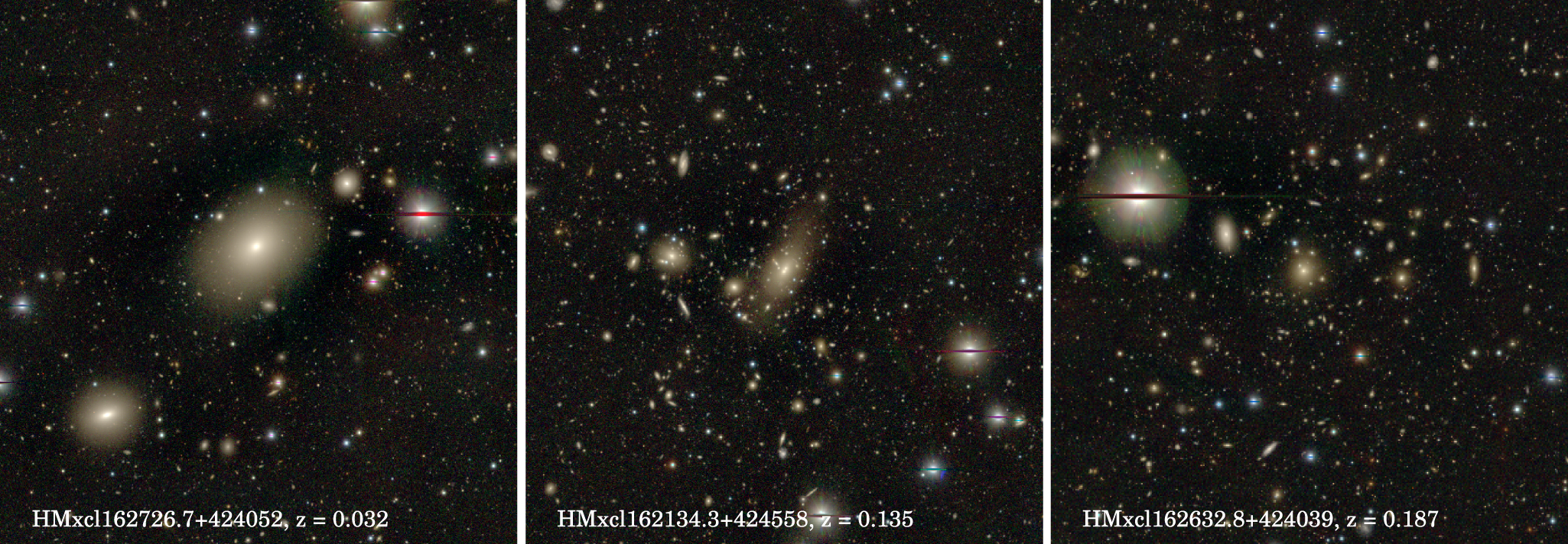
Figure 7 displays examples of three HectoMAP X-ray clusters that lie within the publicly released Subaru/Hyper Suprime-Cam (HSC) imaging footprint. The HSC images clearly demonstrate that the HectoMAP X-ray clusters are generally massive systems containing BCGs surrounded by plenty of members. Even in SDSS images, it is evident that the other HectoMAP X-ray clusters are also massive systems.
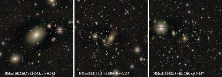
Figure 7. Subaru/Hyper Supreme-Cam images of three HectoMAP X-ray clusters centered on the BCGs of the clusters. The image sizes are 4 arcmin by 4 arcmin. The X-ray centers are near the BCGs.
Download figure:
Standard image High-resolution imageTable 1 lists the properties of the HectoMAP X-ray clusters sorted by redshift. The table contains the cluster ID, the position of the cluster center, the cluster mean redshift, the number of members within the caustics, the center of the extended X-ray emission, the offset between the BCG and the center of the X-ray emission, and the X-ray luminosity. The X-ray luminosity is given in the 0.1–2.4 keV energy band in the cluster rest-frame. Table 2 summarizes the dynamical properties of the HectoMAP X-ray clusters including σcl, R200, and M200. We also list the 1036 cluster members with their redshifts and the redshift source in Table 3.
Table 2. Dynamical Properties of HectoMAP X-ray Clusters
| ID | R200 | σcla | M200 |
|---|---|---|---|
| (Mpc) | (km s−1) | (1014M⊙) | |
| HMxcl162726.7+424052 |

|
257.1 ± 36.7 |

|
| HMxcl141341.6+433925 |

|
307.1 ± 42.9 |

|
| HMxcl162134.3+424558 |

|
963.9 ± 162.4 |

|
| HMxcl151550.0+434556 |

|
458.1 ± 76.4 |

|
| HMxcl162632.8+424039 |

|
654.9 ± 55.0 |

|
| HMxcl142837.5+433852 |

|
708.5 ± 80.9 |

|
| HMxcl150730.7+424424 |

|
450.5 ± 63.2 |

|
| HMxcl163445.9+424641 |

|
586.3 ± 58.0 |

|
| HMxcl150859.8+425011 |

|
435.8 ± 51.3 |

|
| HMxcl153606.7+432527 |

|
555.9 ± 81.2 |

|
| HMxcl143543.4+433828 |

|
567.5 ± 60.9 |

|
| HMxcl163352.9+430529 |

|
192.5 ± 37.1 |

|
| HMxcl141109.9+434145 |

|
673.8 ± 107.3 |

|
| HMxcl145913.1+425808 |

|
507.2 ± 78.6 |

|
| HMxcl132730.5+430433 |

|
810.7 ± 101.1 |

|
Note.
aThe error is the 1σ deviation derived from 1000 time bootstrap resamplings for cluster members within R200.Download table as: ASCIITypeset image
Table 3. Members of HectoMAP X-Ray Clusters
| Cluster ID | SDSS Object ID | R.A. | Decl. | z | zerr | z Source |
|---|---|---|---|---|---|---|
| HMxcl162726.7+424052 | 1237655348358480098 | 246.267148 | +42.509578 | 0.03166 | 0.00001 | SDSS |
| HMxcl162726.7+424052 | 1237655473430135086 | 246.323461 | +42.694233 | 0.03148 | 0.00002 | SDSS |
| HMxcl162726.7+424052 | 1237655473430200607 | 246.571651 | +42.673512 | 0.03168 | 0.00016 | MMT |
| HMxcl162726.7+424052 | 1237655348895285690 | 246.712111 | +42.826501 | 0.03203 | 0.00003 | MMT |
| HMxcl162726.7+424052 | 1237655348895351148 | 246.866560 | +42.806850 | 0.03002 | 0.00002 | SDSS |
| HMxcl162726.7+424052 | 1237655348895416661 | 246.971122 | +42.652934 | 0.03154 | 0.00002 | SDSS |
| HMxcl162726.7+424052 | 1237655348895481992 | 246.958335 | +42.563954 | 0.03148 | 0.00013 | MMT |
| HMxcl162726.7+424052 | 1237655473430331641 | 246.855410 | +42.514434 | 0.03146 | 0.00001 | SDSS |
| HMxcl162726.7+424052 | 1237655473967136890 | 247.216951 | +42.812006 | 0.03158 | 0.00001 | SDSS |
| HMxcl162726.7+424052 | 1237655348895351215 | 246.823539 | +42.695248 | 0.03140 | 0.00001 | SDSS |
Only a portion of this table is shown here to demonstrate its form and content. A machine-readable version of the full table is available.
Download table as: DataTypeset image
Clusters of galaxies are often identified by the red sequence (e.g., Gladders & Yee 2000; Rykoff et al. 2014; Oguri et al. 2017). However, not all galaxies on the red sequence are cluster members (Rines & Geller 2008; Sohn et al. 2017). We examine the color–magnitude diagram for the HectoMAP cluster regions to explore this issue. Figure 8 shows the observed g − r color versus r-band magnitude of the spectroscopically sampled galaxies within 10 arcmin of each HectoMAP X-ray cluster. We identify the red sequence by assuming a slope of −0.04 in color–magnitude space following Rines et al. (2013). We classify objects within ±0.1 of the relation as red sequence members. Among the cluster members identified by the caustic technique, the fraction on the red sequence ranges from 55% to 92%, consistent with previous spectroscopic surveys of massive clusters overlapping this redshift range.
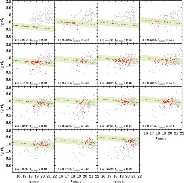
Figure 8. g − r vs. r color–magnitude diagram of the HectoMAP X-ray clusters sorted by redshifts. The red and gray circles show cluster members and spectroscopic targets within 10', respectively. The shaded regions mark the red sequence (dashed line) ± 0.1. frs,mem, the member fraction with respect to the number of spectroscopic targets in the red sequence.
Download figure:
Standard image High-resolution imageAmong the galaxies projected onto the red sequence in the cluster field, the fraction of HectoMAP X-ray cluster members (frs,mem) is remarkably low: 17%–54%, with a median of 36%. The quantity frs,mem is the ratio between the number of spectroscopically identified cluster members and the number of spectroscopic targets on the red sequence. We compute the frs,mem using all cluster members regardless of their apparent magnitude, rather than limited to r ≤ 21.3. The frs,mem changes little when we estimate using the cluster members brighter than the HectoMAP magnitude limit (r ≤ 21.3). The lower membership fraction simply reflects the higher median redshift of the HectoMAP X-ray clusters relative to previous spectroscopic samples where this comparison has been made. Most of the objects that contaminate the red sequence are background.
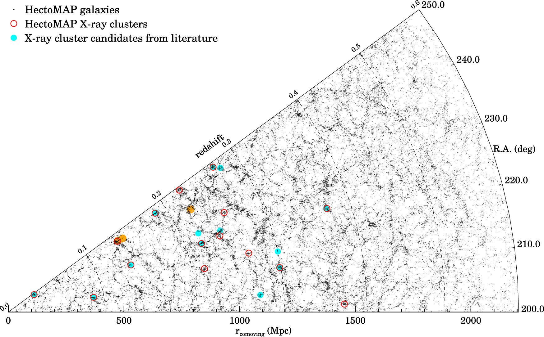
Figure 9 shows a cone diagram for the HectoMAP sample with rpetro,0 < 21.3. The red circles on Figure 9 show the location of the HectoMAP X-ray clusters. For comparison, we also show the positions of previously reported X-ray clusters in the literature (blue circles, see the details in Section 5.1). The HectoMAP X-ray clusters are all embedded in dense structures. On the other hand, many dense structures contain no HectoMAP X-ray clusters, mainly as a result of the lack of extended X-ray extended emission. In a forthcoming paper, we will include the full FoF catalog for HectoMAP and will analyze it in detail (J. Sohn et al. 2018, in preparation). In general, clusters in this catalog mark all of the densest regions in the survey.

Figure 9. Cone diagram for the HectoMAP region. The black dots indicate the HectoMAP red galaxies. The red circles show HectoMAP X-ray clusters. The blue circles mark X-ray cluster candidates from the literature.
Download figure:
Standard image High-resolution image5. Discussion
Combining the dense redshift survey HectoMAP with RASS enables construction of a robust catalog of X-ray clusters. These HectoMAP X-ray clusters contain ∼50 members (median) within the redshift survey (Table 1). The virtue of the cluster survey based on spectroscopic survey data is the reduction of contamination by foreground and background structures. In particular, the caustic method efficiently eliminates non-members along the line of sight.
There are several cluster surveys covering the HectoMAP field, including red sequence detection (e.g., redMaPPer, Rykoff et al. 2014), identification of overdensities based on photometric redshifts (Wen et al. 2009), and identification of X-ray sources in partial overlapping surveys (reference in Table 4). HectoMAP thus provides an opportunity for studying the spectroscopic properties of the clusters in the previous literature (Section 5.2). Sohn et al. (2018) presented an extensive investigation of redMaPPer cluster candidates based on the HectoMAP redshift survey. Here, we limit our discussion to X-ray detected systems (Section 5.1).
Table 4. HectoMAP X-Ray Clusters from the Literature
| ID | R.A.cat | Decl.cat | zcat | R.A.caustic | Decl.caustic | zcaustic | Nmem | fX,lita | LX,litb | fX,ROSAT c | LX,ROSAT d | References |
|---|---|---|---|---|---|---|---|---|---|---|---|---|
| RXC J1627.3+4240e | 16:27:23.6 | +42:40:42.0 | 0.0317 | 16:27:26.7 | 42:40:52.6 | 0.0314 | 33 | 27.50 | 0.06 | 27.50 ± 0.28 | 0.06 ± 0.01 | 1 |
| ABELL1885e | 14:13:46.7 | +43:40:01.6 | 0.0890 | 14:13:43.4 | 43:39:48.2 | 0.0888 | 49 | 52.00 | 1.02 | 34.02 ± 1.36 | 0.66 ± 0.26 | 1, 8 |
| MCXC J1515.5+4346e | 15:15:32.9 | +43:46:35.0 | 0.1370 | 15:15:49.8 | 43:57:25.9 | 0.1342 | 18 | 8.03 | 0.38 | 8.08 ± 0.40 | 0.40 ± 0.20 | 3, 6 |
| ABELL2192e | 16:26:37.2 | +42:40:19.7 | 0.1880 | 16:26:40.5 | 42:39:26.0 | 0.1874 | 61 | 27.50 | 2.73 | 1.16 ± 0.06 | 0.15 ± 0.07 | 1, 8 |
| J150723.2+424402e | 15:07:23.2 | +42:44:02.8 | 0.2173 | 15:07:30.7 | 42:44:17.5 | 0.2184 | 106 | 6.54 | 0.92 | 13.42 ± 0.43 | 1.58 ± 0.51 | 8 |
| J152347.2+434945 | 15:23:47.2 | +43:49:45.9 | 0.2189 | ... | ... | ... | ... | 1.47 | 0.21 | <2.0 | 0.2814 | 8 |
| MCXC J1515.6+4350 | 15:15:36.8 | +43:50:50.0 | 0.2430 | 15:15:15.8 | 43:39:55.2 | 0.2414 | 134 | 6.11 | 1.07 | ... | ... | 3, 4 |
| J163355.8+430528e | 16:33:55.8 | +43:05:28.2 | 0.2699 | 16:33:54.9 | 43:05:45.0 | 0.2705 | 49 | 1.35 | 0.31 | ... | ... | 8 |
| J134117.1+431126f | 13:41:17.1 | +43:11:26.8 | 0.2725 | 13:41:16.3 | 43:11:25.1 | 0.2725 | 24 | 5.73 | 1.33 | <2.7 | 0.6243 | 3, 8 |
| ABELL2198g | 16:28:04.7 | +43:49:25.7 | 0.0800 | 16:28:14.0 | 43:48:57.3 | 0.2767 | 37 | 5.31 | 1.27 | <3.0 | 0.7183 | 7 |
| J141115.4+434123e | 14:11:15.4 | +43:41:24.0 | 0.2980 | 14:11:09.9 | 43:41:45.6 | 0.2998 | 111 | 2.21 | 0.64 | 5.64 ± 0.16 | 1.44 ± 0.40 | 8 |
| VMF98 163 | 14:29:38.1 | +42:34:25.0 | 0.3000 | 14:30:05.6 | 42:51:11.4 | 0.2637 | 47 | 1.84 | 0.39 | <2.0 | 0.4290 | 3 |
| J145912.8+425758e | 14:59:12.8 | +42:57:58.1 | 0.3697 | 14:59:12.0 | 42:58:08.5 | 0.3703 | 34 | 2.26 | 1.06 | 2.96 ± 0.10 | 1.66 ± 0.55 | 8 |
| GHO 1602+4312h | 16:04:25.2 | +43:04:52.7 | 0.8950 | ... | ... | ... | ... | 1.86 | 7.38 | ... | ... | 5 |
| MCXC J1429.0+4241h | 14:29:05.8 | +42:41:12.0 | 0.9200 | ... | ... | ... | ... | 0.91 | 3.87 | ... | ... | 2 |
Notes.
aX-ray flux from the literature in units of 10−13 erg cm−2 s−1. bX-ray luminosity from the literature in units of 1044 erg s−1. cX-ray flux we measure from ROSAT in units of 10−13 erg cm−2 s−1. dX-ray luminosity we measure from ROSAT in units of 1044 erg s−1. eCluster candidates overlapped with the HectoMAP X-ray clusters. fR200 = 0.943 ± 0.006 Mpc, σcl = 485.2 ± 67.9 km s−1, and M200 = 1.248 ± 0.020 × 10¹⁴ M⊙. gR200 = 0.827 ± 0.038 Mpc, σcl = 500.9 ± 70.1 km s−1, and M200 = 0.853 ± 0.094 × 10¹⁴ M⊙. hCluster candidates beyond the redshift range of HectoMAP.References. (1) Böhringer et al. (2000), (2) Horner et al. (2008), (3) Burenin et al. (2007), (4) Vikhlinin et al. (1998), (5) Lubin et al. (2004), (6) Voevodkin et al. (2010), (7) David et al. (1999), (8) Wen et al. (2009).
Download table as: ASCIITypeset image
We investigate the X-ray scaling relation for the HectoMAP X-ray clusters and compare it with relations from the literature in Section 5.2. Finally, we estimate the frequency of X-ray clusters to the depth of RASS in Section 5.3. The cluster masses and X-ray luminosities provide a route to the estimated number density of X-ray clusters over a larger region than has been possible before to this depth. This estimate is a useful guideline for next-generation X-ray surveys (e.g., e-ROSITA).
5.1. Previous X-Ray Cluster Candidates in HectoMAP
To investigate the spectroscopic properties of previously known X-ray clusters in the HectoMAP field, we first search the literature. Several surveys detected X-ray clusters in HectoMAP (Vikhlinin et al. 1998; David et al. 1999; Böhringer et al. 2000; Lubin et al. 2004; Burenin et al. 2007; Horner et al. 2008; Voevodkin et al. 2010). The MCXC catalog (Piffaretti et al. 2011) and the BAX catalog12 facilitated the search. Within the MCXC and the BAX catalogs, we find five and eight X-ray cluster candidates in the HectoMAP field, respectively. The clusters from the MCXC catalog are identified based on ROSAT and those from the BAX catalog are from XMM or ASCA. Some of these clusters overlap, leaving a total of 10 X-ray clusters from the MCXC and BAX catalogs.
Wen et al. (2009) also listed galaxy cluster candidates with X-ray counterparts in the HectoMAP field. Based on SDSS DR6 data, they identified cluster candidates as overdensities within a 0.5 Mpc radius and within the photometric redshift range  . They matched their photometrically identified cluster candidates with the ROSAT point source catalog and provided a list of cluster candidates with X-ray point source counterparts (their Table 2). They identify eight X-ray cluster candidates in the HectoMAP field; three of them overlap the systems from the MCXC and BAX catalogs.
Table 4 lists the 15 X-ray cluster candidates in the HectoMAP field from the literature. The positions and redshifts of clusters are from the literature. The X-ray flux and luminosity are based on the ROSAT band (0.1–2.4 keV). For those objects with X-ray photometry in other bands (e.g., 0.5–2.0 keV), we converted to the ROSAT band using the PIMMS.13 Among 15 cluster candidates from the literature, 8 systems match HectoMAP X-ray clusters.
For the seven remaining cluster candidates, we revisit the previously known X-ray sources that are not associated with HectoMAP X-ray clusters in the RASS data. RASS yields only upper limits on the X-ray fluxes for four systems (Table 4). We do not detect any X-ray flux for three sources, MCXC 1515.6+4350 (Vikhlinin et al. 1998), GHO 1602+4312 (Lubin et al. 2004), and MCXC 1429.0+4241 (Horner et al. 2008).
The previous detections of MCXC 1515.5+4346 and MCXC 1515.6+4350 are confusing. These sources originate from Vikhlinin et al. (1998), who identified two X-ray sources: VMF 168 (R.A., decl., z = 15:15:32.5, +43:46:39, ∼0.26) and VMF 169 (15:15:36.8, +43:50:50. ∼0.14). Later, Burenin et al. (2007) and Voevodkin et al. (2010) listed only one X-ray source (15:15:33.0, +43:46:35) near VMF 168, but at z = 0.137, similar to VMF 169. Indeed, we detect one system (HMxcl151550.0+434556) at z = 0.137; this cluster matches VMF 168 and the X-ray source from Burenin et al. (2007). We suspect that the redshift of VMF 168 listed in Vikhlinin et al. (1998) is incorrect.
We do not identify X-ray emission around VMF 169 in the RASS data. We find an overdensity of galaxies at z ∼ 0.243 near VMF 169, but the center of the overdensity is significantly offset (∼11') from the published location of VMF 169. In conclusion, there is only one significant extended X-ray source at z = 0.137, consistent with the source from Burenin et al. (2007) and Voevodkin et al. (2010).
Figure 10 shows  diagrams for seven previously identified X-ray cluster candidates that lack HectoMAP X-ray cluster counterparts. Because HectoMAP has few redshifts for galaxies with z > 0.6, the
  diagrams at these redshifts do not show structures associated with the reported X-ray sources. The
  diagrams demonstrate that the X-ray cluster candidates from the literature at lower redshift do not always have optical counterparts. We do not find obvious members associated with WHL J152347.2+434945, MCXC J1515.6+4350, and VMF 163. These objects could be matched with foreground or background X-ray sources like quasars. We can calculate caustics for two systems, WHL J134117.1+431126 and Abell 2198. Although the FoF algorithm identifies the two systems, the HectoMAP X-ray cluster catalog does not include these systems because we can measure only the upper limit of X-ray flux based on RASS. We measure σcl and M200 for these systems (see the caption of Table 4).
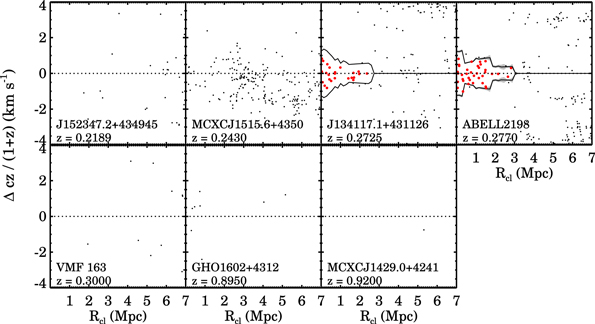
Figure 10.
 diagrams for seven X-ray cluster candidates in the HectoMAP region listed in the literature. The cluster candidates here are not included among the HectoMAP X-ray clusters. The red and black circles show cluster members and spectroscopic targets, respectively. The plots are centered on the known (photometric) redshifts of the cluster candidates. There is no spectroscopic evidence of clusters for three systems: WHL J152347.2+434045, MCXC J1515.6+4350 (VMF 169), and VMF 163. At z > 0.6, the redshift survey is sparse, which limits spectroscopic detection of GHO 1602+4312 and MCXC J1429.0+4241.
Download figure:
Standard image High-resolution imageAbell 2198 is a mysterious case. The redshift of Abell 2198 is reported as z = 0.0798 (Ciardullo et al. 1983; Abell et al. 1989). David et al. (1999) measured an upper limit on the X-ray flux from ROSAT, possibly coincident with this cluster. However, the  diagram shows no distinctive structure at the reported redshift, even though SDSS covers this redshift range quite densely. Instead, we find a cluster at z = 0.277 (shown in Figure 10). The brightest galaxy is offset from the reported center of A2198 by ∼2'.
We suspect that the previously published A2198 redshift was based on redshifts of a few foreground galaxies. Interestingly, Wen et al. (2009) identified this cluster based on photometric redshifts and reported the cluster redshift as zphot = 0.284, remarkably close to the HectoMAP result. Wen et al. (2009) did not find the associated X-ray source perhaps because of the positional offset. Here, we examine the properties of A2198, including X-ray luminosity and velocity dispersion, based on the HectoMAP redshift.
The  diagrams in Figures 6 and 10 provide an estimate of the spectroscopic redshift for most of the X-ray cluster candidates from Wen et al. (2009). The mean cluster redshift offset between the photometric and spectroscopic measures is Δzphot−spec = 0.015 ± 0.008 (∼4500 km s−1). Considering the typical error in the photometric redshifts, the agreement is excellent.
Overall, the census of clusters in the literature contains no additional systems above the RASS flux limit. This result suggests that our catalog construction method yields a complete flux-limited sample. Furthermore, the  diagrams for the X-ray cluster candidates in the literature underscore the importance of cross-checking cluster identification with dense spectroscopy. Some X-ray cluster candidates appear to be false detections, but photometric redshifts do provide cleaner samples when the cluster candidates have an X-ray counterpart (e.g., Wen et al. 2009).
5.2. Cluster Scaling Relation
Figure 11 displays the M200–σcl relation for the HectoMAP X-ray clusters. We also show the relation for the X-ray cluster candidates from the literature. The HectoMAP clusters lie on the trend defined by the larger, lower redshift CIRS (Rines & Diaferio 2006) and HeCS (Rines et al. 2013, 2016) samples.

Figure 11. Velocity dispersion (σcl) vs. M200 (dynamical mass within R200) for the HectoMAP clusters. The red circles show the HectoMAP X-ray clusters and the blue circles display the previously identified X-ray clusters in HectoMAP. For comparison, we show the CIRS clusters (diamonds, Rines & Diaferio 2006) and the HeCS clusters (triangles, Rines et al. 2013). The solid line shows the theoretical relation for the dark matter halo derived from cosmological simulations (Evrard et al. 2008). The gray shaded region indicates the standard deviation of the theoretical relation.
Download figure:
Standard image High-resolution imageWe find two outliers: HMxcl162134.3+424558 with σcl ∼ 963 km s−1 and HMxcl163352.9+430529 with σcl ∼ 193 km s−1. We suspect that poor sampling of the HMxcl162134.3+424558 central region precludes measuring a reasonable velocity dispersion. The second cluster, HMxcl163352.9+430529, is puzzling. The  diagram looks reasonable and the σcl based on 54 members should be robust. The low velocity dispersion of this system may be due to poor sampling of the central region or an anisotropy of this system, (i.e., we observe this cluster along its minor axis). A denser redshift might provide a better understanding of the low σcl for this cluster.
Because the M200 of a cluster is correlated with the velocity dispersion of cluster members, the tight correlation between M200 and σcl is expected. We compare the dynamical properties of HectoMAP X-ray clusters to the theoretical relation given in Evrard et al. (2008), who derived the relation from the simulated dark matter halos. The observed clusters match the model remarkably well. Rines et al. (2013) argued that this agreement supports the accuracy of cluster masses measured from caustic technique.
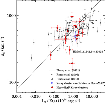
Figure 12 shows the velocity dispersion of the HectoMAP X-ray clusters as a function of their rest-frame X-ray luminosities within the ROSAT band. For comparison, we plot the CIRS and HeCS clusters that are in a similar redshift and mass range.
Figure 12. Velocity dispersion (σcl) vs. X-ray luminosity (LX) for the HectoMAP clusters. The red circles show the HectoMAP X-ray clusters and blue squares indicate previously identified X-ray clusters in HectoMAP. The gray diamonds and triangles display the CIRS clusters (Rines & Diaferio 2006) and the HeCS clusters (Rines et al. 2013), respectively. The solid line shows the best-fit relation for nearby X-ray cluster samples (Zhang et al. 2011). Two low σ clusters are discussed in Section 5.2.
Download figure:
Standard image High-resolution image
The solid line in Figure 12 shows the scaling relation for local clusters from Zhang et al. (2011). This local scaling relation is consistent with the HeCS clusters at a higher redshift range (0.1 < z < 0.3). The HectoMAP X-ray clusters generally follow the LX–σcl relation defined by previous samples and scaling relations.
We note above that the X-ray emission of HMxcl141341.6+433925 (z = 0.089, σcl ∼ 307 km s−1) is contaminated by a soft X-ray source. Thus, the X-ray flux may be overestimated by a factor of two. With this correction, the system moves onto the overall distribution defined by the other systems.
The HectoMAP clusters lie on the previously determined scaling relations between CIRS and HeCS samples. The combination of the sample from the literature with the sample we identify represents the first X-ray sample identified with a dense, large-area redshift survey to this depth. The sample is thus a basis for estimating the number of extended X-ray sources in the RASS data that might be co-identified as candidates with existing photometric surveys like the HSC (Aihara et al. 2017) and Dark Energy Surveys (Dark Energy Survey Collaboration et al. 2016) and then tested with spectroscopy.
5.3. Abundance of X-Ray Clusters
The combined spectroscopic and X-ray surveys provide an estimate of the total number of X-ray clusters on the sky. To the ROSAT detection limit, ∼3 × 10⁻¹³ erg s−1 cm−2, we identify 15 clusters within 53 deg2 corresponding to a number density of ∼0.3 deg−2. Thus, over the entire sky, we expect ∼12,000 ± 3000 clusters.
Schuecker et al. (2004) examined the number of galaxy clusters based on RASS and SDSS early-release data. They identified X-ray cluster candidates from the ROSAT X-ray photon map by applying a likelihood function for their cluster search. They applied a similar likelihood function to the galaxy map from the SDSS photometric catalog for identifying optical cluster candidates. Then, they cross-matched the X-ray and the optical cluster candidates. They used SDSS and redshifts in the NASA/IPAC Extragalactic Database (NED) to estimate the cluster redshift. They identified 75 cluster candidates to the X-ray flux limit ∼3–5 × 10⁻¹³ erg s−1 cm−2 in the ROSAT energy band 0.1–2.4 keV based on a sky coverage of ∼140 deg2 within z ≤ 0.5. Their estimate suggests that there are ∼4000 X-ray cluster candidates to the X-ray flux limit in the total SDSS sky coverage (∼7000 deg2, for their calculation), yielding ∼22,000 ± 2600 systems in the entire sky.
The XXL cluster survey (Pacaud et al. 2016) provides another large X-ray cluster sample for estimating the number of cluster to a limiting X-ray flux. The XXL survey is based on deep XMM-Newton data covering a total area of 50 deg2. Pacaud et al. (2016) identified 100 X-ray extended sources to an X-ray flux limit 3 × 10⁻¹⁴ erg s−1 cm−2, an order of magnitude fainter than RASS. They obtain spectroscopic redshifts of most clusters from various spectroscopic observation campaigns. The redshift range of the XXL clusters is z < 1.2 and the median number of spectroscopic members per XXL cluster is only ∼6.
The XXL cluster sample includes more clusters than the HectoMAP X-ray cluster sample because the X-ray flux limit is deeper. When we limit the XXL flux limit to the HectoMAP X-ray limit, there are 22 XXL clusters with z < 0.4, comparable to the HectoMAP sample. Based on the XXL cluster survey, there would be ∼18,000 ± 4000 X-ray systems over the entire sky to this limit.
The total number of X-ray clusters we predict is marginally consistent with the prediction based on Pacaud et al. (2016), but significantly smaller than the estimate of Schuecker et al. (2004). Our cluster identification method differs from these studies. We require that the system be identifiable in redshift space. This requirement removes superpositions that can masquerade as overdensities on the sky. Thus, we might expect a somewhat smaller number of systems. Cosmic variance may contribute to the marginal agreement between HectoMAP and XXL. Among the three samples, Pacaud et al. (2016) have by far the deepest X-ray data. The inconsistency between the larger-area Schuecker et al. (2004) survey and the smaller HectoMAP X-ray and Pacaud et al. (2016) samples requires further investigation based on large independent catalogs.
6. Summary
HectoMAP is a dense redshift survey covering the redshift range z ≲ 0.7. The survey is sufficiently dense that massive clusters of galaxies can be identified in redshift space throughout this range. As a step toward constructing a complete catalog of systems we compare a FoF catalog with RASS to identify extended X-ray sources. We also cross-identify the X-ray systems with the available Hyper Suprime-Cam imaging of the HectoMAP region. The images confirm the robustness of the cluster identification.
We identify 15 massive galaxy clusters (7 are new) based on combining HectoMAP with the RASS. We apply an FoF algorithm to identify systems in redshift space and cross-identify the ROSAT X-ray extended emission. The clusters we identify contain ≳20 spectroscopically identified members. The cluster survey is complete to the X-ray flux limit of ∼3 × 10⁻¹³ erg s−1 cm−2. We also publish 1036 redshifts for the cluster members.
We also revisit known X-ray cluster candidates from the literature based on the HectoMAP spectroscopic sample and the RASS. We find no additional clusters above the flux limit, suggesting that our flux-limited sample is complete. Among the candidate systems in the literature, four are not confirmed by the spectroscopic data. These X-ray sources may be contaminated by background AGNs. This test underscores the importance of dense spectroscopic samples for identifying galaxy clusters with multi-wavelength data.
The HectoMAP X-ray clusters generally follow the scaling relations derived from known massive X-ray clusters: M200–σcl and LX–σcl relations. A few poorly sampled systems are outliers.
Our cluster survey predicts ∼12,000 ± 3000 detectable X-ray clusters in RASS with ∼3 × 10⁻¹³ erg s−1 cm−2 and within z ≲ 0.4. To the same flux limit, our prediction is consistent with a prediction based on the XXL survey (Pacaud et al. 2016), but is significantly below the prediction by Schuecker et al. (2004). The e-ROSITA flux limit should resolve this issue and will enable detection of massive clusters throughout the HectoMAP redshift range, along with a much greater cluster mass range at redshifts ≲0.4. The combination of HectoMAP dense spectroscopy, complete Subaru imaging of the entire HectoMAP field, and the e-ROSITA survey should provide a robust catalog of clusters for increasingly sophisticated tests of cluster evolution and for determination of the cosmological parameters.
We thank an anonymous referee for a careful reading of the manuscript that improved the clarity of the paper. The referee kindly pointed out a mistake in Table 1. J.S. gratefully acknowledges the support of the CfA Fellowship. M.J.G. is supported by the Smithsonian Institution. G.C. and H.B. acknowledge the support by Deutsche Forschungsgemeinschaft through the Transregio project TR33 and through the Excellence Cluster "Origin and Evolution of the Universe." A.D. acknowledges partial support from the INFN grant InDark. We thank Susan Tokarz for reducing the spectroscopic data and Micheal Kurtz, Perry Berlind, and Mike Calkins for assisting with the observations. We also thank the telescope operators at the MMT and Nelson Caldwell for scheduling Hectospec queue observations. We thank the HSC help desk team, especially Michitaro Koike and Sogo Mineo, for making tools available. J.S. acknowledges Felipe Andrade-Santos for his help in using PIMMS. This research has made use of NASA's Astrophysics Data System Bibliographic Services.
We have made use of the ROSAT Data Archive of the Max-Planck-Institut für extraterrestrische Physik (MPE) at Garching, Germany. This research has made use of the X-Rays Clusters Database (BAX), which is operated by the Laboratoire d'Astrophysique de Tarbes-Toulouse (LATT), under contract with the Centre National d'Etudes Spatiales (CNES).
The Hyper Suprime-Cam (HSC) collaboration includes the astronomical communities of Japan and Taiwan, and Princeton University. The HSC instrumentation and software were developed by the National Astronomical Observatory of Japan (NAOJ), the Kavli Institute for the Physics and Mathematics of the Universe (Kavli IPMU), the University of Tokyo, the High Energy Accelerator Research Organization (KEK), the Academia Sinica Institute for Astronomy and Astrophysics in Taiwan (ASIAA), and Princeton University. Funding was contributed by the FIRST program from Japanese Cabinet Office, the Ministry of Education, Culture, Sports, Science and Technology (MEXT), the Japan Society for the Promotion of Science (JSPS), Japan Science and Technology Agency (JST), the Toray Science Foundation, NAOJ, Kavli IPMU, KEK, ASIAA, and Princeton University.
This paper makes use of software developed for the Large Synoptic Survey Telescope. We thank the LSST Project for making their code available as free software at http://dm.lsst.org.
The Pan-STARRS1 Surveys (PS1) have been made possible through contributions of the Institute for Astronomy, the University of Hawaii, the Pan-STARRS Project Office, the Max-Planck Society and its participating institutes, the Max-Planck Institute for Astronomy, Heidelberg and the Max-Planck Institute for Extraterrestrial Physics, Garching, the Johns Hopkins University, Durham University, the University of Edinburgh, Queens University Belfast, the Harvard-Smithsonian Center for Astrophysics, the Las Cumbres Observatory Global Telescope Network Incorporated, the National Central University of Taiwan, the Space Telescope Science Institute, the National Aeronautics and Space Administration under grant No. NNX08AR22G issued through the Planetary Science Division of the NASA Science Mission Directorate, the National Science Foundation under grant No. AST-1238877, the University of Maryland, and Eotvos Lorand University (ELTE), and the Los Alamos National Laboratory.
This work is based on data collected at the Subaru Telescope and retrieved from the HSC data archive system, which is operated by Subaru Telescope and Astronomy Data Center at the National Astronomical Observatory of Japan.
Footnotes
- 8
- 9
- 10
Deblending of a contaminated cluster X-ray source can generally be performed for the following cases: (i) the sources are clearly separable and the cluster source can be identified from the coincidence with the concentration of galaxies in the optical, (ii) the non-cluster source is clearly identified by a local contamination with a different spectral hardness ratio (see Chon & Böhringer 2012), or (iii) the contaminating source can be clearly identified as a point source superposed on the extended emission from the cluster.
- 11
The calculations are performed using the plasma spectral code xspec available from NASA HEASARC at https://heasarc.gsfc.nasa.gov/xanadu/xspec.
- 12
- 13