


Abstract
The planets of the solar system are neatly divided between those with atmospheres and those without when arranged by insolation (I) and escape velocity ( ). The dividing line goes at
  . Exoplanets with reported masses and radii are shown to crowd against the extrapolation of the solar system trend, making a metaphorical cosmic shoreline that unites all the planets. The
  relation may implicate thermal escape. We therefore address the general behavior of hydrodynamic thermal escape models ranging from Pluto to highly irradiated extrasolar giant planets (EGPs). Energy-limited escape is harder to test because copious XUV radiation is mostly a feature of young stars, and hence requires extrapolating to historic XUV fluences (
 ) using proxies and power laws. An energy-limited shoreline should scale as
  , which differs distinctly from the apparent
  relation. Energy-limited escape does provide good quantitative agreement to the highly irradiated EGPs. Diffusion-limited escape implies that no planet can lose more than 1% of its mass as H2. Impact erosion, to the extent that impact velocities
  can be estimated for exoplanets, fits a
  shoreline. The proportionality constant is consistent with what the collision of comet Shoemaker–Levy 9 showed us we should expect of modest impacts in deep atmospheres. With respect to the shoreline, Proxima Centauri b is on the metaphorical beach. Known hazards include its rapid energetic accretion, high impact velocities, its early life on the wrong side of the runaway greenhouse, and Proxima Centauri's XUV radiation. In its favor is a vast phase space of unknown unknowns.
Export citation and abstract BibTeX RIS
1. Introduction
Volatile escape is the classic existential problem of planetary atmospheres (Hunten 1990). The problem has gained new currency with the discovery and characterization of exoplanets (Borucki et al. 2010; Lissauer et al. 2014). When escape is important, it is likely to be rapid, and therefore is relatively unlikely to be caught in the act, but the cumulative effects of escape should show up in the statistics of the new planets (Owen & Wu 2013; Lopez & Fortney 2014). In this paper we discuss the empirical division between planets with and without apparent atmospheres inside and outside of the solar system. The paper is organized around four figures that compare the planets (dwarf and other) of the solar system to the ∼590 exoplanets that were relatively well characterized as of 2016 August 26. In Section 6 we then address the place of Proxima Centauri b and Trappist 1f among these planets.
In Section 2 we compare total stellar radiation intercepted by a planet (insolation, I) to the planet's escape velocity ( ). In previous work we found that on such a plot the empirical division between planets with and without atmospheres follows a
  power law that we have called the "cosmic shoreline" (Zahnle 1998; Catling & Zahnle 2009; Zahnle & Catling 2013). We then compare the planets to the predictions of two different thermal escape models, one pertinent to small planets with condensed volatiles at the surface, and the other pertinent to giant planets that are close to their stars. We also compare the planets to the water vapor runaway greenhouse limit, which has a different relation to insolation and gravity.
In Section 3 we restrict stellar irradiation to extreme ultraviolet (EUV) and X-rays, here collectively called XUV radiation ( ). The intent is to address the popular XUV-driven escape hypothesis (e.g., Hayashi et al. 1979; Sekiya et al. 1980a, 1981; Watson et al. 1981; Lammer et al. 2003b, 2009, 2013, 2014; Lecavelier et al. 2004; Yelle 2004; Tian et al. 2005; Erkaev et al. 2007, 2013, 2015, 2016; Garcia-Munoz 2007; Koskinen et al. 2009; Murray-Clay et al. 2009; Tian 2009; Koskinen et al. 2013, 2014; Owen & Wu 2013; Lopez & Fortney 2014; Johnstone et al. (2015); Tian 2015; Owen & Alvarez 2016, the list is not complete). We estimate historic XUV fluences of the host stars to find that the shoreline also appears in XUV with the same power law,
  .
.
Section 4 begins by pointing out that the empirical  relation is not in accord with the basic predictions of energy-limited escape. We compare the predictions of the simplest quantitative energy-limited escape model to the apparent planets. Because XUV radiation is well suited to driving the escape of hydrogen in particular, it is natural to discuss selective escape and diffusion-limited escape in the context of XUV-driven escape. We show here that diffusion-limited escape, where applicable, reduces to a general result that may be particularly germane to super-Earths.
Section 5 addresses impact erosion. Impact erosion of planetary atmospheres offers a plausible alternative to thermal or irradiation-driven escape (Zahnle et al. 1992; Zahnle 1998; Catling & Zahnle 2013; Schlichting et al. 2015). Here we compare impact velocities  to escape velocities for the planets plotted in the previous figures. With impact erosion there is a reasonable expectation that a
  relationship should apply at all scales; the difficulty in testing the hypothesis is in estimating what the impact velocities should be.
Section 6 addresses Proxima Centauri b (which we refer to as "Proxima b" for the rest of the paper because the star, which is uniquely the Sun's nearest neighbor, should really be just "Proxima"). In Section 6 we document how we plot Proxima b against the other planets and discuss its place with respect to the cosmic shoreline.
2. Total Insolation versus Escape Velocity
Figure 1 plots relative insolation I against escape velocity  for the adequately characterized planets. The figure shows that atmospheres are found where gravitational binding energy is high and total insolation is low. The figure also shows that the boundary between planets with and without apparent atmospheres is both well defined and follows an empirical
  power law that extends from the planets of our solar system up through the known exoplanets.

Figure 1. Atmospheres are found where gravity—here represented by the escape velocity—is high and insolation—here represented by the total stellar insolation at the planet relative to that received by Earth—is low. The presence or absence of an atmosphere on solar system objects is indicated by filled or open symbols, respectively. Extrasolar planets with known masses and radii as of 2016 August, 26 (Schneider et al. 2011, http://exoplanet.eu) are also plotted. The extrasolar planets are presented as blue disks if Saturn-like ( ), as green boxes if Neptune-like (
 ), as red diamonds if Venus-like (
 ), and as orange squares if none of the above (
 ). The simple
  power law bounding the cosmic shoreline is drawn by eye. Several of the more outlandish worlds are labeled by name; abbreviations like "138b" refer to "Kepler 138b." Error bars on the extrasolar planets are omitted for clarity. Planets that are plotted to the left of the
  power law may have very uncertain
  or they may be airless. Several models are also shown for comparison. Hydrodynamic thermal escape models for CH4, N2, and H2O assume vapor pressure equilibrium at the surface. The two H2O curves are for escape as H2O (solid) or as H2 (dashed). The magenta line is the thermal stability limit for hot extrasolar giant planets (EGPs), as described in Section 2.4. The curvature is caused by tidal stripping. Also shown is the runaway greenhouse threshold for steam atmospheres. The models are described in the text. Proxima b is plotted in gold at three times (10 Myr, 100 Myr, now) in the luminosity evolution of Proxima. Trappist 1f is plotted at three times (10 Myr, 100 Myr, now).
Download figure:
Standard image High-resolution imageFor most solar system objects we use escape velocities from Zahnle et al. (2003). The Kuiper Belt objects (KBOs) and Pluto/Charon have been updated to reflect more recent information (Rabinowitz et al. 2006; Brown & Schaller 2007; Pál et al. 2012; Braga-Ribas et al. 2013; Brown 2013; Fornasier et al. 2013; Lellouch et al. 2013; Wesley et al. 2013; Stern et al.2015). The presence or absence of an atmosphere for solar system objects is indicated by filled or open symbols, respectively. For the solar system, what is meant by "having an atmosphere" is usually pretty obvious, but even here there are borderline cases, such as Io, which has a very thin volcanogenic SO2 atmosphere. The KBOs are more ambiguous. A few of the largest retain stores of frozen methane on their surfaces. These are plotted in purple on Figure 1 as half-full boxes. It is reasonable to suppose that their surface volatiles will evaporate when close to the Sun, and they will then for a time have atmospheres similar to those of Pluto and Triton. This sort of seasonal transformation is very likely for Eris, which is currently near aphelion, and rather unlikely for Sedna, which is rather near its perihelion.
Figure 1 includes the nearly complete roster of transiting exoplanets with published radii and masses as of 2016 August, 26. For these planets, orbital parameters, diameters, and stellar luminosities are measured, albeit not always very precisely. With the exception of Kepler 138c and 138d, we have not attempted to weight the catalog by the purported quality of the data. A few planets have been omitted because we were unable to estimate insolation. The exoplanet.eu database (Schneider et al. 2011, http://exoplanet.eu) was filtered to include only exoplanets with (i) a reported radius R; (ii) a reported mass M; and (iii) a reported orbital period P. Radii and masses were used to compute escape velocities  . For most of the exoplanets the measured diameters and densities are typical of giant planets, which indicates that most of the transiting planets plotted in Figure 1 have atmospheres. Planets with radii
  —Saturns and super-Saturns—are plotted as blue disks. Planets with radii
  —Neptunes and sub-Saturns—are plotted as dark blue disks. Exoplanets with radii
  —sub-Neptunes, Earths, and super-Earths—are plotted as green diamonds. This particular sorting by size appears to have some basis in fact (Lopez & Fortney 2014), with the three categories loosely corresponding to H2-rich planets, H2O-rich planets or H2-enveloped rocky planets, and rocky planets.
For stellar luminosity we use the stellar radii R⋆ and stellar effective temperatures T⋆ listed for most of the central stars in the exoplanet.eu database,

When one or both of R⋆ and T⋆ is not listed, we estimate stellar luminosity using the visual magnitude mv and stellar distance d (in parsecs) as reported in the exoplanet.eu database,

Here mv = 4.83 is the visual magnitude of the Sun at 10 pc. For a few of the planets, neither  nor
nor  can be computed; these planets we omit. Insolation I is plotted as a dimensionless ratio relative to what is incident on Earth today. Insolation is computed using the planet's reported semimajor axis a if available, otherwise we estimate a from the stellar mass M⋆ and the period P,

in order to compute

where a⊕ is the semimajor axis of Earth's orbit.
The general pattern seen in Figure 1 is what one would expect to see if escape were the most important process governing the volatile inventories of planets. Where the gravitational well is deep (measured by escape velocity), or where the influence of the central star is weak (measured here by insolation), planetary atmospheres are thick. Where the gravity is weak or the star too bright, there are only airless planets. It is curious that the non-giant planets in our solar system that have atmospheres seem to be strung out along a single  line, rather than scattered over the half-space below and to the right of the bounding line. A second surprise is that the known transiting EGPs crowd against the extrapolation of that line. The
  line spans two orders of magnitude in escape velocity and nearly eight orders of magnitude in insolation. It is remarkable that a single power law should appear to relate hot EGPs at one extreme to Pluto and Triton at the other.
What Figure 1 does not show is what one might expect to see if the presence of atmospheres depended mostly on local nebular temperature (during accretion) or volatile supply. To put this another way, small warm worlds with significant atmospheres are missing. Such worlds are permitted if not mandatory in supply side scenarios; indeed, active comets provide extreme examples of what such worlds can look like during their brief lives.
2.1. Thermal Escape from Icy Planets
We consider isothermal atmospheres in which the major gas is in vapor pressure equilibrium with condensed volatiles at the surface. We call these Clausius-Clapeyron (CC) atmospheres because they are controlled by vapor pressure (Lehmer et al. 2017). Clausius-Clapeyron atmospheres are fairly common in the solar system, with Pluto, Triton, and Mars being notable examples. Our model resembles an earlier Jeans escape model used by Schaller & Brown (2007) and Brown (2012) to address thermal escape from Kuiper Belt objects. The chief difference is that we are addressing much faster escape rates, conditions where Jeans escape would be misapplied. Perez-Becker & Chiang (2013) investigated similar models for evaporation of very hot silicate planets. Limitations and uncertainties stemming from the isothermal approximation along with some alternative approximations to planetary winds that may seem more realistic are discussed in Section 9, and examined in more detail in the Appendices.
Isothermal hydrodynamic escape is described in terms of the isothermal sound speed  , where Tc is the temperature and m is the mean molecular mass of the atmosphere. Pressure p is that of a perfect gas
  with density ρ. The outflow is described in spherical (radial) geometry in steady-state by continuity,

where u is the outflow velocity and r is the radial coordinate increasing outward, and by the force balance of inertia, pressure, and gravity,

in which M is the mass of the planet and G is the universal gravitational constant. These can be combined into a single isothermal planetary wind equation,

In a strongly bound atmosphere,  and
and  near the surface, so that
  . At large radii the geometric term
  term eventually surpasses the gravity term, and the right-hand side of Equation (7) changes sign. At the critical distance rc where
  , zeroing the left-hand side of Equation (7) requires either that
  or that
  . The unique solution with
  , in which the velocity is equal to the sound speed
  at the critical point
  , is the critical transonic solution for the wind and is the physical solution, provided that the ram pressure of the wind
  at the critical point exceeds any background pressure exerted by interplanetary space.
Equation (7) is easily integrated for the upward velocity at the surface, us, in terms of the isothermal temperature Tc and the critical point conditions. Where escape is modest and  ,
,

gives a good approximation to us. The density and pressure at the surface of a CC atmosphere are determined by the saturation vapor pressure at the surface temperature Ts,

For display in Figure 1 we use empirical expressions for the vapor pressures of CH4, N2, and H2O given by Fray & Schmidt (2009). For the isothermal CC atmosphere, the rate of mass loss is a function of Ts and us

The other determining equation is the balance between the power absorbed from sunlight and the sum of power radiated in the thermal infrared and power spent evaporating, heating, and lifting warm gas to space,

where α is the Bond albedo, which for icy worlds we take as  . The rightmost term takes into account the latent heat of vaporization Lv, an important part of the energy budget for small icy bodies. Here we are interested in whether a planet can hold an atmosphere for billions of years. In these cases escape is slow enough that the terms in Equation (11) involving
  are negligible, so that the surface temperature is just the effective temperature.
Empirically, upper atmospheres of the CH4-rich planets in the solar system are roughly twice as hot at high altitudes as they are at the surface (Table 1). The upper atmospheres are warm because (i) CH4 absorbs sunlight and (ii) CH4 photolysis produces organic molecules and hazes that absorb sunlight, but at low temperatures neither CH4 nor the hazes radiate as effectively as they absorb. The upper atmosphere temperatures are higher on Uranus and Neptune because the background gas is H2, so that additional radiative coolants are limited to hydrocarbons like C2H2. On Titan, Triton, and Pluto, the background gas is N2, which enables production of a wider variety of more efficient radiative coolants, HCN especially. For the CH4–N2 atmospheres of icy worlds we let reality be a guide and approximate the atmospheric temperature with  .
.
Table 1. Surface Temperatures and Mesosphere Temperatures of CH4-rich Atmospheres
| Planet | Surface Ts | Mesosphere Tc |

|
References |
|---|---|---|---|---|
| Titan | 94 | 150–190 | 0.50–0.63 | Koskinen et al. (2011) |
| Triton | 38 | 50–60 | 0.63–0.76 | Olkin et al. (1997) |
| Pluto | 42 | 72 | 0.6 | Gladstone et al. (2016) |
| Uranus | 60a | 110–150 | 0.4–0.55 | Marten et al. (2005) |
| Neptune | 60a | 110–150 | 0.4–0.55 | Marten et al. (2005) |
Note.
aThese are the effective temperatures.Download table as: ASCIITypeset image
The black and green curves labeled "CH4" and "N2" are evaporation lines for the small icy planets. The density is set to  g cm−3, similar to the densities of Triton, Titan, Ganymede, Callisto, and Pluto. The curves are computed for a star of age
  billion years and an atmophile mass fraction
  , where
  . It is interesting that the nominal curves "CH4" and "N2" resemble what is actually seen in the solar system. However, the results shown here are quite sensitive to
  (the sound speed, squared), and consequently they are insensitive to everything else. We can regard the CC model as a descriptive model, in the sense that it provides a plausible explanation of what is observed, but it may prove difficult to implement as a prescriptive model, because in general Tc and m are hard to predict theoretically.
The solid blue curve is the comparable  evaporation line for H2O from planets scaled from volatile-enriched versions of Earth (
 ,
,  ), Europa (
 g/cm3,
  ), and Ganymede (
 ,
,  )—by chance, these three cases are nearly indistinguishable in this plot, so we show them as one curve. For these models we set Tc = Ts as, unlike the case for N2-CH4 atmospheres, we know of no good reason nor have we seen much evidence to suggest that the upper atmospheres of watery worlds should be especially hot or cold.
The blue water line is to the asteroids as the methane line is to the KBOs, whether by accident or design, but unlike the case for the methane line, which approaches Pluto, Triton, and Titan, the water line comes nowhere close to explaining the terrestrial planets. The water line can be moved into the vicinity of the terrestrial planets by raising  by an order of magnitude. This can be done either by converting the H2O into H2 or by invoking a hot upper atmosphere. The result of raising
  is illustrated by the dashed blue curve, computed from the same CC model as for water but with
  . Such a model may also be relevant to Hayashi-like primary nebular atmospheres, as it is reasonable to anticipate chemical equilibration and exchange between H2, H2O, and silicates at the surface if the atmosphere is deep (Hayashi et al. 1979; Sekiya et al. 1980a, 1981; Ikoma & Genda 2006).
2.2. The Water Vapor Runaway Greenhouse
The runaway greenhouse threshold is expected to be a weak function of planetary parameters. To illustrate, assume that the runaway greenhouse limit is set by a troposphere saturated with water vapor becoming optically thick (Nakajima et al. 1992). In the absence of pressure broadening, optical depth τ will scale as the column depth; with pressure broadening, this will be multiplied by the pressure to a power ξ on the order of unity (Pollack 1969; Robinson & Catling 2012; Goldblatt et al. 2013; Robinson & Catling 2014). For a pure water vapor atmosphere, these considerations imply that (Goldblatt 2015)

where κ is an opacity. If we approximate the vapor pressure of water by a simple exponential

with Tw = 6000 K and  bars, the runaway greenhouse limit should scale as

an expression that is well approximated over the range of interest by  . The surface gravity g is expressed in terms of
  and planet density ρ by
  . This leaves

This relation is plotted with  and
and  in Figure 1 as the "H2O runaway greenhouse." GCM-based estimates of the onset of the runaway range between 1.1 to 1.7 solar constants, with details of cloud structure and cloud physics and planetary rotation responsible for much of the variance (Abe et al. 2011; Leconte et al. 2013a, 2013b; Wolf & Toon 2015; Way et al. 2016). The range of uncertainty is encompassed by the thickness of the plotted line.
2.3. The Moon
Figure 1 shows the Moon rising above the intersection of the water lines. In all likelihood, the apparent desiccation of the Moon is a memory of how the Moon was made rather than the ruin of a more promising world, but as plotted here, the Moon as a habitable world appears to be marginally unstable against both thermal escape and the runaway greenhouse. Today, most of the lunar surface is unstable to Jeans escape of water (e.g., Catling & Kasting 2017). When viewing the Moon from the viewpoint of terraforming it, both problems would be made more tractable by providing abundant heavy ballast gases to reduce the atmosphere's scale height.
2.4. Extrasolar Giant Planets
Here we address thermal evaporation of EGPs. The topic has been addressed many times (e.g., Owen & Wu 2013) with much more sophisticated models than we employ here, but for our purposes, it seems best to hold to the isothermal approximation, which has the advantage of being analytic and easy to work with. Models of silicate-rich gas giants have tended to predict warm or even hot upper atmospheres, because small molecules made of rock-forming elements such as TiO are better absorbers of visible light than they are emitters of thermal infrared radiation. However, early reports of thermal inversions on hot Jupiters (e.g., on HD 209458b; Burrows et al. 2007; Knutson et al. 2008) have since been cast into doubt by analyses of more precise data of higher spectral resolution (Line et al. 2016). A difference from the icy worlds is that these planets are close enough to their stars that tidal truncation must be taken into account. This is conveniently done in terms of the Hill sphere distance, which is defined by

where as above, a refers to the star-planet distance and M⋆ to the mass of the star (Erkaev et al. 2007). Along the star-planet axis, Equation (6) becomes

and Equation (7) becomes

Equation (18) assumes spherical symmetry for tidal forces, which is not a good assumption. Its crudeness is probably comparable to treating irradiation as globally uniform or the temperature as isothermal. The critical point is found by solving the cubic for rc,

Equation (18) is easily integrated analytically,

Note that u(r) is independent of density. Near the surface, where  , Equation (20) can be rewritten as an equation for the flow velocity at the surface us using the critical point conditions. The flux at the surface
  is obtained by multiplying by the surface density
  ,
,

To use Equation (21) requires choosing  at the lower boundary using other information.
In EUV- and XUV-driven escape studies, the lower boundary is typically set at the homopause or at the base of the thermosphere, with the latter defined by a monochromatic optical depth in XUV radiation (e.g., Watson et al. 1981; Tian et al. 2005; Lammer et al. 2013). The homopause can be a reasonable a priori choice if escape is sluggish enough that a homopause exists. However, as we show below in Section 4.2, for a gas giant to evaporate in 5 Gyr, the flux of hydrogen to space is too great by orders of magnitude for a homopause to exist. In a full-featured hydrocode simulation of an XUV-heated wind, the lower boundary condition can be justified a postiori as self-consistent for a particular model by showing the model to be insensitive to changing it (e.g., Watson et al. 1981; Murray-Clay et al. 2009; Owen & Alvarez 2016).
In the simplest picture, a gas giant does not have a well-defined surface. Under these conditions, the whole planet takes part in the flow to space, with the source of the escaping gas being the shrinking or rarefaction of the interior. To first approximation, all EGPs have roughly the same radius; the typical radius of a hot Jupiter is 84,000 km (Fortney et al. 2008). Constant radius is a property of polytropes with a  equation of state. The radius is
  , where G is the Newtonian gravitational constant (Hubbard 1973). Using observed radii of the known roster of transiting planets gives
  cm5 g−1 s−2. The interior is described by an analytic solution,

We set the lower boundary where the inner polytrope and the outer isothermal envelope meet; i.e., where the polytropic pressure equals the pressure of an ideal gas at the planet's effective temperature  . This gives

The other equation pertinent to escape is the global energy balance,

The terms involving  are the work done against gravity and any excess heat left in the gas as it escapes. As was the case in Section 2.1 above, if thermal escape is extended over 5 billion years, the
  terms in Equation (24) are negligible, and Equation (24) reduces to the usual expression for effective temperature,

For the EGPs we set the Bond albedo  ,
,  ,
,  , and in keeping with the isothermal assumption, we set
  . The magenta curve in the upper right-hand region of Figure 1 is computed for complete evaporation of the planet in
  Gyr; i.e., we solve Equations (21), (23), and (24) for
  such that
  . The simple model bounds the population of EGPs (blue disks) rather nicely. We stress that this is not an XUV-driven escape model. The planet evaporates because the planet is thermally unstable, not because XUV heating is removing the outer atmosphere.
3. XUV-driven Escape
Stellar EUV and X-ray radiation can be very effective at driving the escape of H and H2 from young planets (Hayashi et al. 1979; Sekiya et al. 1980a). Urey (1952) put it succinctly: "Hydrogen would absorb light from the Sun in the far-ultraviolet and since it does not radiate in the infrared [it] would be lost very rapidly." Urey (1952) regarded hydrogen escape as obvious and an essential process in planetary evolution (and of a habitable Earth in particular), but he did not quantify it. Hayashi et al. (1979) proposed that massive hydrogen-rich atmospheres of young planets were removed by copious EUV ("extreme ultraviolet,"  nm) and X-ray (
 nm) radiations from young stars (Sekiya et al. 1980a, 1981). Hayashi's idea has proved fruitful, and subsequent work on EUV and X-ray driven escape has been voluminous (see Tian (2015) and Catling & Kasting (2017) for recent reviews). EUV and X-ray radiations are usually linked in the literature as XUV radiation because they are expected to be related in stars. We use the XUV notation here.
In practice, it is challenging to test the XUV hypothesis because the bulk of the XUV that a star emits in its lifetime is emitted when the star is very young, and hence for all but the youngest exoplanets, the relevant stellar XUV fluxes are not observables. Rather, each star's ancient XUV flux needs to be reconstructed from imperfectly known empirical relationships that link stellar age and spectral type with observed XUV emissions. For our purposes, the matter is made fuzzier by the uncertainty that surrounds the fiducial star—our Sun—as different extrapolations differ markedly for the Sun when young.
Lammer et al. (2009) scaled XUV fluxes both with age and with spectral type for F, G, K, and M stars. They give two part power laws of the general form  , with relatively shallow slopes (
 ) before 0.6 Gyr and relatively steep slopes (
 ) thereafter. In this prescription, the cumulative XUV flux is a well-defined integral dominated by the saturated phase. We performed these integrals and generalized their result to a simple power law,

which we then express in normalized form for plotting on Figure 2 as

The scaling in Figure 2 is therefore with respect to a model of the total cumulative XUV radiations emitted by the ancient Sun, including the early saturated phase.

Figure 2. Analog to Figure 1 for estimated cumulative XUV irradiation, which is often hypothesized to be the driving force behind planetary evaporation (Tian 2015). Uncertainties are much larger here than in Figure 1 because all the XUV fluences need to be reconstructed, including the normalizing XUV fluence for Earth. No attempt is made to estimate errors for planets outside the solar system. The  line is drawn by eye. The dashed magenta curve is for XUV-driven energy-limited escape from tidally truncated hot EGPs. It is labeled by fractional mass lost,
  . The model is described in Section 4.3 below. Proxima b and Trappist 1f are plotted as described in Sections 6 and 7 below.
Download figure:
Standard image High-resolution imageNot surprisingly, Figure 2 looks much like Figure 1, since only the exoplanets have been changed. It is interesting that the EGPs (blue disks) in particular form a tighter distribution, which may be a hint that with XUV we are on the right track. The  line is drawn in by hand to guide the eye. The dashed magenta curve represents the quantitative predictions of a basic XUV-driven escape model to be described below in Section 4.3. The XUV-driven escape model works rather well for EGPs.
4. XUV-driven Escape: Part II
In this section we address the expected form an energy-limited power law would take, and compare its predictions to those of XUV-driven escape (Figure 3).

Figure 3. Here the data from Figure 2 are plotted against the expectations of the simplest theory. Energy-limited models predict that if tidal stripping is unimportant, the insolation  should be linearly proportional to the quantity
  . Here we express x as normalized to Earth,
  , so that Earth sits at
  . The green diagonal lines represent a family of these predictions, denoted in the plot by the relative fraction
  of the planet's mass that can be lost in XUV-driven escape. The upper green line
  is the extension of the dashed magenta curve for XUV-driven energy-limited escape from tidally truncated hot EGPs. The middle (solid) green line
  approximates the upper bound (
 ) on diffusion-limited escape of H2 for systems that are a few billion years old. The lower (dashed) green line
  approximates the upper bound on diffusion-limited escape of H2 if rapid escape is restricted to young XUV-active stars. Proxima b and Trappist 1f are plotted as described in Sections 6 and 7 below.
Download figure:
Standard image High-resolution image4.1. General Considerations
It is possible to quantify the predictions of the XUV hypothesis if the escape is energy limited. Energy-limited escape is expected if the XUV radiation is too great for the incident radiation that can be thermally conducted to the lower atmosphere (Watson et al. 1981). If tidal truncation is neglected for the moment, the energy-limited escape can be expressed as

where  is an efficiency factor that is usually taken to be
  (e.g., Lammer et al. 2013; Owen & Wu 2013; Koskinen et al. 2014; Bolmont et al. 2017). The mass-loss efficiency η is lower than the heating efficiency (fraction of incident XUV energy converted into heat) because the escaping gas is hotter, more dissociated, and more ionized than it was before it was irradiated. The factor η is a function of T, being smaller in cooler gas (<3000 K) in which
  is a major radiative coolant (Koskinen et al. 2014) and smaller in hot gas (
 K) in which collisionally excited Lyα is a major coolant (Murray-Clay et al. 2009). In a steam atmosphere, the far-ultraviolet (FUV,
  nm) can also be important because it is absorbed by H2O, O2, and CO2, provided irradiation is modest enough to leave the molecules intact (Sekiya et al. 1981). The contribution of the FUV is implicitly folded into η. The total mass loss

is obtained by integrating the star's XUV radiation history expressed in terms of the Sun's history using  . For the XUV history of the Sun itself, we follow Ribas et al. (2005, 2016),

where  ,
,  , and where

is the saturated upper bound on the Sun's youthful excess. Cumulative escape is then

which can be rearranged as a linear relation between  and x
and x

with x defined by

Results are plotted in terms of the parameter x in Figure 3 for  as green lines and labeled for a range of lost masses
  . As in Figure 2, we apply
  to the data in order to present a single relation that spans all the planets. The solar system is fit by
  , a trend that does not extend to the exoplanets, which are better matched by
  .
.
4.2. Diffusion-limited Escape
The diffusion-limited flux gives the upper bound on how quickly hydrogen can selectively escape by diffusing through a heavier gas that does not escape; more properly, it is the upper limit on the difference between hydrogen escape and heavy-constituent escape. It is often thought of in the context of vigorous hydrogen escape driven by XUV radiation (Sekiya et al. 1980b; Zahnle & Kasting 1986; Hunten et al. 1987), but it is quite general (Hunten & Donahue 1976). The diffusion-limited flux regulates hydrogen escape or H2 abundance on Venus, Earth, Mars, and Titan today (see review by Catling & Kasting 2017). It is likely that, should the diffusion-limited flux be lower than the energy limit, the H2 mixing ratio  will increase until the two limits are equal, as seen on Titan and Mars. If
  , and the energy limit still exceeds the diffusion limit, it is not obvious what happens. The atmosphere may either escape as a whole (although the heavier gases escape more slowly, so that the remnant atmosphere becomes mass fractionated), or hydrogen escape is throttled to the diffusion limit and the excess energy is radiated to space by the heavy gases. A possible example of escape at the diffusion limit among the EGPs is HD 209458b (Vidal-Madjar et al. 2003, 2004; Yelle 2004; Koskinen et al. 2013).
The upper bound on the escape flux of a gas species of molecular mass mi from a static gas atmosphere of molecular mass mj ( ) in the diffusion limit from an isothermal atmosphere is

where fi is the mixing ratio of the light gas and bij is the binary diffusion coefficient between the two species i and j. Typically,  . The corresponding mass-loss rate is

The timescale for losing an atmosphere of mass  is
is  . The upper bound that diffusion places on atmospheric escape can be written

It is notable that this ratio is very nearly independent of planetary parameters—i.e., this constraint is the same for all planets. For H2 escaping through N2,  , for which

with  measured in Gyr. This means that it is difficult for a planet to selectively lose more than about 0.5% of its mass as H2 in 5 Gyr, even if H2 is a major constituent (
 ), as it often appears to be on exoplanets. In many XUV-limited escape scenarios, the time available for energy-limited escape is shorter than a few hundred million years, which reduces the maximum differential H2 loss to less than 0.05% of the planet's mass. Whether this is an important constraint depends on several factors. If H2 is overwhelmingly abundant and the heavy gases are inefficient radiative coolants, they can be carried along, and
  becomes the difference between H2 escape and heavy gas escape (Sekiya et al. 1981; Zahnle & Kasting 1986). If the heavy gases condense, they can be separated from H2 by precipitation and the gas diffusion limit does not apply. But for warm planets with considerable reservoirs of volatiles other than H2, the constraint may set the boundary between planets that evolve to a vaguely Earth-like state versus those that never progress past a vaguely Neptune-like state. That XUV-driven escape should lead to such a bimodal distribution of planets is an observation that has also been made on the basis of the limited XUV energy available (Owen & Wu 2013).
4.3. Extrasolar Giant Planets
The simple linear relation between  and x in Equation (33) does not apply for the close-in planets that are afflicted by tidal truncation. For these we need to include the Hill sphere terms, which break the
  relation. For these planets we start with a tidally truncated XUV-heated energy-limited escape flux,

As above, we treat EGPs as all having the same radius R. With R held constant, M can be replaced by  the star-planet distance a can be replaced by
  and M⋆ is replaced M⊙ by expressing
  , in which the stellar mass–luminosity relationship is conveniently written in the form
  . With these relations, the
  ratio cancels out of Equation (39). The resulting expression between
  and
and  should hold approximately for all main-sequence stars and their giant planets,

Equation (40) is readily solved for  as a function of
  . Results are plotted for
  with
with  as the dashed magenta lines in Figures 2 and 3. For the particular case with R held constant,
  , so the curves are uniquely defined in both plots. As has been pointed out by others (e.g., Owen & Wu 2013), the quantitative predictions made by the simple XUV model are good enough to be intriguing.
5. Impact Erosion
Impact erosion of planetary atmospheres can be another path to ruin (Walker 1986; Melosh & Vickery 1989; Zahnle et al. 1992; Zahnle 1993, 1998a; Griffith & Zahnle 1995; Chen & Ahrens 1997; Brain & Jakosky 1998; Newman et al. 1999; Genda & Abe 2003, 2005; Catling & Zahnle 2009; Korycansky & Zahnle (2011); de Niem et al. 2012; Catling & Zahnle 2013; Schlichting et al. 2015). The basic idea is that a portion of a planetary atmosphere is blasted into space if an impact is large enough and energetic enough. Once in space, the noncondensing volatiles are presumed dispersed by radiation pressure or the solar wind, while condensing materials are for the most part swept up again. In detail, how impact erosion actually works remains a work in progress. It may be that impact erosion is mostly caused by very large collisions that drive off much of the atmosphere in a single blow (Korycansky 1992; Chen & Ahrens 1997; Genda & Abe 2003, 2005), or it may be more like sandblasting, with tens of thousands of small impacts each doing a little (Walker 1986; Melosh & Vickery 1989; Zahnle et al. 1992), or it could be something in between, or a combination of all these effects. Moreover, impact erosion cannot be evaluated while not also evaluating the impact delivery of new volatiles.
In previous work, we suggested that impact erosion is likely to be dominated by numerous relatively small projectiles striking the planet's surface at velocities well in excess of the escape velocity, while impact delivery of new volatiles is likely to be dominated by a few slow-moving very large volatile-rich bodies (Zahnle et al. 1992; Griffith & Zahnle 1995). Consequently, although the loss of atmosphere by impacts may be plausibly approximated by a continuous function, impact delivery of volatiles is likely to be profoundly stochastic. If this is how it works, impact erosion, when it gets the upper hand, will annihilate the atmosphere, because as the atmosphere thins, the eroding projectiles become ever smaller and more numerous. This kind of impact erosion is a good candidate for creating a nearly airless world like Mars (Melosh & Vickery 1989; Zahnle 1993), and it readily accounts for the sharp distinction between the atmospherically gifted Titan on one hand and the airless Callisto and Ganymede on the other (Zahnle et al. 1992; Griffith & Zahnle 1995; Zahnle 1998). But where by chance a single late great impact delivers an atmosphere so massive that all subsequent impacts are insufficient to remove it, a considerable atmosphere can be left on a planet where one might not expect to find one (Griffith & Zahnle 1995). If impact erosion is the chisel that sculpts extrasolar systems, we would expect that by chance there will exist a few small, close-in planets enveloped in appreciable atmospheres. This may be germane to assessing Proxima b.
However it happens, it is plausible that the efficiency of impact erosion should scale as  , and therefore we plot in Figure 4 the planets on the grid
  versus
  . To prepare Figure 4, we use solar system impact velocities from Zahnle et al. (2003) with appropriate updates for the KBOs. For the exoplanets we assume that the impacting bodies come from prograde orbits of modest inclination and eccentricity that generically resemble those of the asteroids and Jupiter-family comets that strike Earth and Venus. In the inner solar system, encounter velocities
  are typically on the order of 0.5–1.0× the orbital velocity, with the higher encounter velocity appropriate to matter falling from greater heights above the Sun (i.e., comets) (Bottke et al. 1995). The circular orbital velocity
  of an extrasolar planet is computed using the reported period and either the semimajor axis, such that
  , or the star's mass M⋆, such that
  . For most planets, a and M⋆ are both listed; for these we take the average. What is actually plotted in Figure 4 uses

with  .
.

Figure 4. Here typical impact velocities, estimated from the orbital velocities  of the planets, are plotted against
  . The shaded area in the lower right is unphysical; we plot it this way because it looks nice. Solar system bodies with atmospheres, such as Earth, are plotted in solid colors. Bodies in the solar system that are devoid of atmospheres are plotted with open gray symbols. Kuiper Belt objects are purple. Transiting exoplanets are plotted as blue disks (Saturns and Jupiters), green boxes (Neptunes), and red diamonds (Venuses). Expansive error bars are omitted for clarity. The empirical impact erosion stability limit for solar system atmospheres is roughly
  . Proxima b (in gold) and Trappist 1f (charcoal) are plotted twice. The higher impact velocity presumes bodies from distant orbits; with Proxima, this could mean bodies that orbit α Centauri. The lower impact velocity presumes bodies in prograde orbits roughly coplanar with the planets. Low impact velocities might be expected in the Trappist 1 system.
Download figure:
Standard image High-resolution imageAlthough the data are very uncertain, Figure 4 clearly shows that impact erosion cannot be lightly dismissed. We are currently not in a position to make quantitative predictions comparable to those we made for insolation-driven escape, we do not know the actual impact velocities anywhere other than in our own solar system, and even here we meet with considerable dispersion; neither do we know the volatile contents of the impacting bodies; we have no robust theory of how impact erosion works; nor do we have a robust theory to describe the retention and loss of the delivered volatiles. What we can say is that impact erosion has promise as a global explanation, and because its effects are roughly parallel to those of insolation-driven escape, the two processes might often work together. For what it is worth, the empirical dividing line for the ensemble,  , is at a higher
  than the
  that had been discussed for Mars (Melosh & Vickery 1989; Zahnle 1993). It may be germane that the ejecta from comet Shoemaker–Levy 9 were launched at 20%–25% of the impact velocity (Zahnle 1996), which suggests to the optimist that the relation
  may hold generally for airbursts in deep atmospheres. This in particular is a topic that should be addressed in future work.
6. Proxima b: On the Beach
In 2016, a planet somewhat more massive than Earth was discovered orbiting the Sun's nearest neighbor every 11.2 days (Anglada-Escudé et al. 2016). The planet lies within the conventional habitable zone, in that it intercepts a total amount of insolation comparable to what the Earth intercepted during its inhabited Archean Eon ca. 3 Ga ago. This mix of qualities—the nearest exoplanet, vaguely Earth-massed, in the habitable zone—almost guarantees that Proxima b will be explored by humans or their descendants at some point in the distant future. There has been a fair amount written about Proxima b that does not all need to be repeated here (Anglada-Escudé et al. 2016; Davenport et al. 2016; Ribas et al. 2016; Turbet et al. 2016; Barnes et al. 2017; Coleman et al. 2017; Goldblatt 2017; Meadows et al. 2017). Here we wish to document how we plotted Proxima b in Figures 1–4 and then, briefly, we speculate about its habitability.
6.1. Proxima b: Escape Velocity
Proxima b's escape velocity is uncertain because we do not know its radius; we do not know whether it is a globe of air, water, earth, or metal. The radial velocity gives  . We presume the median nominal mass of
  . If rocky, using
  (Zeng et al. 2016), we estimate
  km s−1. To set a rough upper uncertainty, we take a more face-on
  orbit, for which
  km s−1. To set a rough lower uncertainty, we presume that Proxima b is ice-rich with a bulk density half that of a rocky world of the same mass, for which
  km s−1.
6.2. Proxima b: XUV Heating
For Proxima specifically, Ribas et al. (2016) estimate both the current and the cumulative relative XUV irradiations of Proxima b and Earth. For the present, they estimate that  . For the cumulative total, they estimate that
  . We plot both estimates in Figures 2 and 3, each with a factor 3 uncertainty. In Figure 2, Proxima b appears relatively vulnerable to XUV-driven escape. Only a large and dense Proxima b orbiting an XUV-quiet Proxima plots with the terrestrial planets of our solar system. Otherwise, Proxima b plots with the least of the extrasolar Neptunes and a few other smaller planets. When the ensemble is replotted according to the expectations of energy-limited flux, however, Proxima b looks rather ordinary (Figure 3). Figure 3 also suggests that Proxima b at 0.05 au has intercepted enough XUV energy to drive off about 1% of its mass; a water-world Proxima b should be durable to XUV radiation if it could be made in the first place, but a more Earth-like hydrosphere could be vulnerable to being wholly lost.
6.3. Proxima b: Insolation
After it formed, Proxima is presumed to have slowly faded to the main sequence like any small M dwarf. Figure 1 shows insolation levels from Ribas et al. (2016) at three times: when Proxima was just 10 Myr old, when Proxima was 100 Myr old, and today. With respect to total insolation, Proxima b is much like Earth or Venus in Figure 1. As Ribas et al. (2016) and Barnes et al. (2017) and many others have pointed out, when Proxima was young, insolation exceeded the runaway greenhouse threshold at Proxima b's current 0.05 au distance for the first ∼150 Myr or so of their mutual existence (Barnes et al. 2017). This means that Proxima b, if it had water when young, would have held it initially in the form of steam, which eliminates the cold trap as a bottleneck to hydrogen escape. (Other ways to eliminate the cold trap as a bottleneck to escape is to make water vapor a major constituent, as can happen if other gases are scarce (Wordsworth & Pierrehumbert 2013), or to invoke a so-called "moist greenhouse" stratosphere, the reality of which is in active debate (Kasting 1988; Kasting et al. 2015; Leconte et al. 2013a; Wolf & Toon 2015).) If hydrogen escape is restricted to the runaway greenhouse epoch, estimates of the total XUV-driven energy-limited escape range from less than an Earth ocean of water Ribas et al. (2016) to 3–10 oceans (Barnes et al. 2017), a difference that can be attributed to assumptions about Proxima as a young star.
6.4. Proxima b: Oxygen
It has been suggested that if the source of escaping hydrogen is water, O2 might build up in the atmosphere at the diffusion-limited rate, and if the hydrogen from several oceans of water escaped, it might be possible for hundreds of bars of O2 to accumulate in the atmosphere that is left behind (Luger & Barnes 2015; Schaefer et al. 2016; Barnes et al. 2017). However, these models do not account for atmospheric photochemical reactions between oxygen and hydrogen that can reduce the H2 mixing ratio and thus throttle hydrogen escape. For example, the hydrogen escape rate from Mars is currently very slow because the strong negative feedback between oxygen and hydrogen ensures that both are lost from the atmosphere in the 1:2 ratio of the parent molecule (Hunten & Donahue 1976). The same 1:2 ratio holds for oxygen and hydrogen escape from Venus today (Fedorov et al. 2011). Moreover, iron in a vigorously convecting mantle has the capacity to consume thousands of bars of O2. For example, Gillmann et al. (2009) and Hamano et al. (2013) dispose of the excess oxygen generated by hydrogen escape from Venus's accretional steam atmosphere by placing it into the mantle while still mostly molten under a steam atmosphere. In any event, O2 on Venus has yet to be detected (Fegley 2014). Schaefer et al. (2016) include aspects of the kinetics of the mantle sink. If the XUV is very large, hydrogen escape can in principle be vigorous enough to drag the oxygen that is liberated by water photolysis into space (Zahnle & Kasting 1986; Luger & Barnes 2015; Schaefer et al. 2016). For example, Zahnle & Kasting (1986, Figure 8) showed that for conditions germane to a steam atmosphere on Venus, molecular diffusion ensures that oxygen escape must exceed the surface sink on oxygen, no matter how efficient the latter. Schaefer et al. (2016) reached a similar conclusion for GJ 1132b and other worlds. When hydrogen escape exceeds the diffusion limit, the diffusion limit becomes the rate at which oxygen is left behind to oxidize the planet or accumulate in the atmosphere. However, in addition to not including atmospheric chemistry, neither model took into account that because the mixed wind is heavier, it must be hotter than pure hydrogen and thus has more power to cool itself radiatively.
6.5. Proxima b: Impacts and Impact Erosion
The history and nature of impacts experienced by Proxima b are almost wholly conjectural (Coleman et al. 2017). Still, impacts happen. It may be helpful to divide impactors into three general classes: (i) material co-orbital with Proxima b; (ii) material in orbits about Proxima (analogous to the Sun's asteroid and Kuiper belts), and (iii) material in orbits about α Centauri A or B or both (Kuiper belts and Oort clouds would be solar system analogs). The first category is swept up very quickly and is better regarded as part of Proxima b's accretion; this is addressed separately below. In the second category we imagine bodies in prograde orbits roughly coplanar with Proxima b and perturbed from relatively distant orbits, with aphelia at 1 au, into highly elliptical Proxima b-crossing orbits. By analogy to impacts on Earth (Bottke et al. 1995), we estimate that typical encounter velocities would be on the order of  , which corresponds to
  km s−1. The third category is analogous to the comets and asteroids that strike the Galilean satellites (in mildly hyperbolic orbits with respect to Jupiter), with almost all of the velocity of the stray body attributable to the gravitational well of the central body. We have previously modeled this scenario for the Galilean satellites, taking into account the distribution of impact probabilities associated with the distribution of encounter orbits (Zahnle et al. 1998b). Generalizing from Zahnle et al. (1998b), we estimate that close encounters of the third kind would fall in the range
  i.e., we estimate that
  km s−1. Cases (ii) and (iii) are plotted on Figure 4. It is apparent at a glance that Proxima b is more vulnerable to the negative consequences of impacts than are Earth and Venus, a not surprising observation that has been anticipated (cf. Lissauer 2007; Raymond et al. 2007). We conclude that almost all the collisions that matter to impact erosion and impact delivery must be from debris orbiting Proxima itself, at velocities that are marginally more erosive than what we see in the inner solar system.
6.6. Proxima b: Accretional Heating
If averaged over 100 Myr, the energy of accretion of a planet like Earth is comparable in magnitude to the insolation received over that same period. This was very important for Earth and Venus because they likely accreted on a 30–100 Myr timespan, and the added energy of accretion pushed both planets above their runaway greenhouse limits (Matsui & Abe 1986; Abe & Matsui 1988; Zahnle et al. 1988; Hamano et al. 2013). For Earth, the steam atmospheres were episodic transients after large impacts, but Venus's steam atmosphere was probably irreversible, and hence led directly to the profound desiccation of Venus's atmosphere and mantle (Hamano et al. 2013).
By contrast to Earth and Venus, Proxima b could have accreted very quickly. Lissauer (2007) showed that in basic Safronov accretion theory, habitable zone (HZ) planets of small M dwarfs are expected to accrete in less than 105 years, orders of magnitude faster than Earth or Venus. Accretion in 105 years implies a surface temperature of 2000 K if airless and perhaps 4000 K if the planet had an atmosphere, which at temperatures like these it most certainly would have had (Lupu et al. 2014). In its potential for rapid accretion, Proxima b is more like a Galilean satellite than a solar system planet. The comparable accretion time for Europa is 200 years, which scarcely seems credible for a small world that retains much water, to say nothing of icy Callisto, accreting in just 3000 years, yet never fully melting. Evidently, Europa's and Callisto's accretions were governed by the supply of new matter from the Sun's accretion disk to Jupiter's accretion disk, rather than by the properties of Jupiter's accretion disk. The ruling timescale then becomes that of forming the solar system as a whole, which appears to have been on the order of 3 million years (and slow enough to preserve a cold Callisto). But Proxima b is much bigger than Europa or Callisto. Even if material were supplied to the Proxima system from an unknown source on a more leisurely 10 million year timescale, Proxima b's accretion would not only be too rapid for water to condense, it would be too rapid for a magma surface to freeze solid unless there were no atmosphere (Lupu et al. 2014).
6.7. Proxima b: Stellar Wind
Here we ask if atmospheric erosion by Proxima's stellar wind has been important. In the solar system, the solar wind erodes through direct collisions (sputtering) and through its magnetic field (ion pickup). The latter in particular is important for Venus and Mars. Venus intercepts about 4000 grams of solar wind per second, estimated using  yr−1 (Wood et al. 2002). Average quiet-Sun observed rates of oxygen ion escape from Venus are much lower, about 150 g
  (Fedorov et al. 2011). Modeled O+ escape rates range from 150 to 800 g
  (Jarvinen et al. 2009). Escape driven by the solar wind at Mars is more efficient: Mars intercepts about 300 grams of solar wind each second, which is comparable to the observed O+ escape rate of 160 g
  (Brain et al. 2015) and to modeled O+ escape rates of 300–500 g
  (Lammer et al. 2003a). Apparently the solar wind impinging on Mars roughly erodes its own mass in Martian gas although Venus suggests that escape processes are, among other things, sensitive to
  .
.
Suppose that the observed Martian regime approaches the asymptotic efficiency. This may be a reasonable bound on a process that in broad brush is a problem of turbulent mixing. If so, the planet's mass-loss rate would be equal to the mass of stellar wind intercepted,

where  is the star's mass-loss rate. The stellar wind is assumed to be strong enough that the planet's cross-section to the wind is comparable to its physical cross-section. Proxima b therefore intercepts
  of
of  . We estimate that
  for Proxima today is roughly
  yr−1, in which we have scaled the solar wind by XUV (Wood et al. 2002). If we assume that
  , we estimate that Proxima b has intercepted roughly
  g of stellar wind since it first became potentially habitable at 150 Myr of age. This corresponds to
  of Proxima b's mass, or about 10 bars of atmosphere. Losses would be smaller than 1 bar if the extrapolation were based on Venus. These estimates are respectively 2 and 3 orders of magnitude smaller than what XUV can do in the first 150 Myr for an H2-rich or H2O-rich atmosphere (Barnes et al. 2017). On the hand, the stellar wind might pose the greatest existential threat to a CO2 atmosphere at times after the first 150 Myr.
6.8. Proxima b: "Ashes, Ashes and Dust, and Thirst there is"
Proxima b may have no good analog in the solar system. Venus seems the best candidate. Venus retains very little water (in the atmosphere,  of Earth, Fegley 2014) and probably very little in its interior. Gillmann et al. (2009) and Hamano et al. (2013) explain Venus as having been thoroughly desiccated by hydrogen escape from a steam atmosphere over a molten silicate surface that lasted for more than 100 Myr. In this picture, the mantle remained in equilibrium with the water vapor in the atmosphere, and thus the loss of all the water from the atmosphere also meant the loss of almost all the water from the mantle. Both early insolation and accretional energy are greater for Proxima b than for Venus, which makes Venus's story seem all too likely Proxima b's story as well.
Mercury and Io represent end members where the forces of escape (for Mercury, insolation and XUV; for Io, impact erosion and thermal radiation from Jupiter when young) are almost wholly victorious. Both retain sulfur. Notably, Mercury appears to retain about as much water as it can harbor in its shadowed craters, which is empirical evidence either that late high-speed impacts by comets or asteroids do not wholly preclude the accretion of small amounts of water, or that even a planet as blasted as Mercury can still degas a little water. Mars may be a guide to what Proxima b might look like if it were in equilibrium with a late bombardment (post-dating the runaway greenhouse phase) of volatile-rich bodies dislodged from cold distant orbits. Between Mercury and Mars there is a place for a habitable desert state for Proxima b (Abe et al. 2011; Turbet et al. 2016).
Europa and Ganymede are examples of planets born with too much water to lose. We argued with respect to Figure 3 that over 5 Gyr it is difficult for any planet, no matter how small or strongly irradiated, to selectively lose more than about 0.2% of its mass as hydrogen, so that an initial water inventory greater than 2% of the planet's mass is likely not to be lost save by impact erosion. Both Europa and Ganymede appear to have been heated well enough during accretion to be thoroughly differentiated, yet each retains large amounts of water. How a water-world Proxima b might accrete is a puzzle—perhaps a giant impact of a stray water-rich planet with a local planet could do it, or perhaps it migrated in from a colder place in what is to date a wholly conjectural planetary system—but given the current absence of a predictive model of planet formation, nothing should be ruled out (Lissauer 2007; Ribas et al. 2016; Barnes et al. 2017; Coleman et al. 2017).
Earth would be the best of all possible analogs, but the real Earth hydrosphere is too thin to have survived Proxima's youthful luminosity and the onslaught of XUV radiation and flares that continues today (Davenport et al. 2016). Both Ribas et al. (2016) and Barnes et al. (2017) explicitly construct habitable states by starting with just enough water that the loss of the hydrogen from some 1–10 oceans of water leaves an ocean or so behind after the early steam atmosphere condensed. A decade ago, Lissauer (2007) had pointed out that an Earth-like outcome in this scenario, or in any of several other scenarios he considered, requires "precisely the right amount of initial water or just the right dynamics." This means that Earths are unlikely outcomes for Proxima b compared to a vastly greater phase space of less happy outcomes. When conceiving Kepler, Borucki et al. (1996) set out to determine the number of Earth-like planets in the cosmos by direct observation. With all apologies to theory, this remains the path forward.
7. Trappist 1f
Seven Venus-sized planets were recently discovered orbiting the very faint M-star Trappist 1 (Gillon et al. 2017). Several of these are in the habitable zone. One of the planets, Trappist 1f, has already been well-enough characterized by transit-timing variations that it cannot be ignored. Trappist 1f has therefore been superposed on Figures 1–4. Interest ensures that other planets in the system will also soon be well characterized, but we pass on these here to return to the topic in the future if merited.
Trappist 1 is described as a red dwarf of effective  , mass
  , and luminosity
  (Gillon et al. 2017). A naïve comparison to models by Burrows et al. (2001) would suggest that it could be young, ∼0.5 Gyr, and still fading, but it is more likely that the star has reached its asymptotic main-sequence luminosity and is therefore older than 1 Gyr. In either case, the star would have been about 4 times brighter than it is now at 100 Myr and about 20 times brighter when 10 Myr of age (Figure 1). Trappist 1f's current orbit spent more time in the runaway greenhouse zone than did Proxima b's.
The star's strength as a UV (Bourrier et al. 2017) and X-ray (Wheatley et al. 2017) source have been reported; we take  , a factor 3 or so lower than X-ray saturation. Even allowing for the fading of L⋆, the ratio of the cumulative XUV fluence to that from the Sun is probably no more than the current ratio of XUV fluxes. We plot Trappist 1f at the current ratio in Figures 2 and 3. Trappist 1f's imaginary atmosphere appears distinctly more vulnerable to XUV radiation in Figures 2 and 3 than does Proxima b's.
We consider two cases for impact erosion in Figure 4: a lower impact velocity for material that might be exchanged between planets ( ), and a higher impact velocity (
 ) for the Trappist 1 equivalent of a Kuiper Belt or Oort cloud. Other things being equal, Trappist 1f's position resembles the position of Proxima b rather closely with respect to impacts.
Trappist 1f is roughly the same size as Earth but has a distinctly lower density, reportedly just 60 ± 17% that of Earth (Gillon et al. 2017). It is tempting to do this with ice, in the general pattern of Europa. Indeed, the Trappist 1 system as a whole does resemble Jupiter and its Galilean satellites, both in scale and in relative masses. The Jupiter system is characterized by a regular pattern of densities. Water has clearly acted as a volatile, either in the materials from which the moons formed, or perhaps it has migrated from the inner to the outer moons in response to the luminosity of young Jupiter. But the solar system provides another possible analog. At Saturn, the densities of the small icy satellites are seemingly random, falling in the sequence (1.15, 1.62, 0.97, 1.49, 1.25) g/cm−1 as one marches outwards from Mimas to Rhea. This behavior is probably a consequence of collisional evolution, with little sign that water has acted as a volatile. A similarly random pattern of densities in the Trappist 1 system would suggest that Trappist 1f is best seen as an analog of Tethys, as iron-poor as Tethys is rock-poor.
8. Some Outliers
Kepler 138 is an M dwarf with three known planets. The planets 138c and 138d are the same size ( ), but of markedly different masses. The masses themselves are considerably uncertain, but their ratio is not: Jontof-Hutter et al. (2015) report
  with 68.3% confidence. The solar system pairs Mercury/Moon (iron/rock), Io/Callisto (iron-rock/rock-ice), and Enceladus/Tethys (rock-ice/ice) all have density ratios within a factor two, which suggests that it may be difficult to achieve a factor of 3 by accident. Both planets are in the runaway greenhouse zone, and thus water is not condensible. Giving 138d an H2 atmosphere can help, but asking this system to conform to photoevaporation will not be straightforward. A possibility that may seem promising is to invoke chemistry. If 138c were an iron-rich body, we should expect Fe and H2O to react to make an H2-dominated atmosphere with a huge scale height, while in 138d we might imagine a rocky or watery body (Jontof-Hutter et al. 2015) with a H2O-CO2 atmosphere and a scale height ten times smaller. Under these conditions, the atmosphere of the denser planet would be more vulnerable to escape.
The planets Kepler 36b and 36c present a similar challenge. The two planets are in closely adjacent orbits circling an evolving (brightening) subgiant star. The outer planet (c) is about 70% more massive and almost 300% more voluminous. The densities differ by a factor of ten. To first approximation, the smaller planet is a super-Earth and the larger planet is a sub-Saturn or a gassy Neptune. Owen & Morton (2016) devised a photoevaporation scenario in which the two planets were initially of similar composition, but the inner planet, less massive from the start, evaporates first, and the authors showed that this could be made to work. Curiously, it is now the smaller of the planets that has the higher escape velocity and the deeper potential well, which probably requires that the interior of the inner planet was much hotter during escape than it is now. Of course it is also possible that they were just made this way, however.
All three known planets of Kepler 51 (b, c, and d) are reported to be of exceedingly low density (Masuda 2014). They are outliers in Figures 1–4. These planets as described are not really stable, and thus there is cause for some skepticism of their reported attributes (Cubillos et al. 2017). Masuda (2014) reports a considerable uncertainty in the diameter of the star. It is possible that the star has been misunderstood.
9. A Discussion of Isothermal Escape
The isothermal approximation is (i) simple; (ii) consistent with  radiative cooling; (iii) equally applicable to all planets; and (iv) only one of several crude approximations we have made to poorly constrained factors that are important to escape, and it is probably not the worst of them. The isothermal approximation raises two different questions. One is how well the isothermal approximation describes the wind, and the other is how well an isothermal wind approximates the thermal escape rate.
In principle, the first question—the detailed temperature structure of the planetary wind—is answerable only through direct observations of planetary winds. Lacking these, models can be constructed that contain more physics. Detailed modeling of this sort is far beyond the scope of this paper. What we can address within the scope of the paper is whether the energy required by isothermal escape contradicts the assumption of isothermal escape.
We here used isothermal models to estimate escape rates from small planets with condensed surface volatiles at one extreme, and for highly irradiated EGPs at the other extreme. For the former, we show in detail in Appendix A that the energy needed to remove a planet's volatiles on astronomical timescales of tens or hundreds of millions years, timescales appropriate to Figure 1, is small compared to the energies associated with radiative heating and cooling. Figures 5 and 6 of Appendix A are illustrative examples made by moving famous dwarf planets to warmer places.

Figure 5. Left: Energy required to maintain an isothermal state in a water vapor atmosphere escaping from a warm Europa, as a function of height (black curve), compared to the available energy sources. Isothermal Europa loses its ocean in 30 Myr. The total FUV+XUV radiation absorbed is shown at three levels of solar activity, with 1× being the modern Sun. The curve labeled IR is thermal emission from the surface absorbed by water vapor in the low-pressure limit. Right: Energy required by an isothermal atmosphere escaping from a warm Pluto (black curve). The atmosphere is predominantly N2, with 1% CH4 and 10 ppmv of C2H2. Alternative Pluto loses a volatile inventory equal to 1% of its mass in 100 Myr. For the modern Sun, isothermal escape is almost exactly balanced by XUV+FUV heating. Higher levels of UV would make the atmosphere hotter, or would need to be balanced by radiative cooling if the isothermal approximation is to hold.
Download figure:
Standard image High-resolution image
Figure 6. Global energy required by escape (solid black curve), compared to some other energy terms pertinent to escape. The example depicts a continuum of evaporating Europas with different surface temperatures. The black dashed curve indicates how long it takes for each Europa to lose its ocean if escape is isothermal. The total absorbed FUV+XUV radiation is computed using the isothermal water vapor atmosphere for  . The stellar FUV+XUV heating is high in part because the absorbing volume of the atmosphere is vastly larger than Europa itself. The curves labeled "advected thermal energy" and "thermal conduction" are indicative of the order of magnitude of these terms in non-isothermal atmospheres. Thermal conduction is shown, but it is negligible because the distances are large and the temperature gradients are small. The curve labeled "IR" is a lower bound on the absorption of thermal emission from the surface. No radiative transfer is performed. The purpose here is merely to show that the energy that is exchanged by radiative transfer exceeds the energy spent boosting gas into space.
Download figure:
Standard image High-resolution imageFor the EGPs, temperatures in the upper atmosphere are universally expected to be much hotter than the underlying atmosphere because no effective means of cooling the gas have been identified at temperatures below 104 K (e.g., Koskinen et al. 2014). Thus escape from EGPs is often approximated as limited by the XUV energy, with a base near a homopause set at the top of the underlying mixed atmosphere. Where this may fail is that, because escape of 104 K hydrogen is relatively easy, the thermosphere may not be the true bottleneck to escape. Instead, the bottleneck may be at the homopause, which is controlled by the magnitude of turbulent mixing, which in turn is controlled by the total energy flux moving through the planet. The isothermal approximation by contrast includes the entire atmosphere in escape, and it involves all the incident sunlight. For the isothermal model, the bottleneck is at the bottom of the isothermal zone. The upgrade to the isothermal model would be a more supple stratospheric temperature profile generated by an accurate treatment of radiative transfer, which of course depends on the detailed chemical and particle composition of the atmosphere and the radiative properties of the hot gases and particles at the temperatures and pressures of the stratosphere; we will not go there. It is a curious coincidence that the two end-member models—the energy-limited flux and isothermal escape—predict essentially the same scenario when applied to planetary evaporation (compare Figures 1 and 2), but it should be noted that both models heavily depend on tidal forces to truncate the atmosphere, so that tidal truncation may be the true control. If so, a more accurate description of the tidal potential would be the direction in which to take further research.
The second consideration—how well an isothermal wind approximates the escape rate—is addressed in Appendix B by comparing isothermal escape to escape predicted by some tractable alternative temperature structures for the exemplary small ocean world. For this purpose, we construct polytropic planetary winds that are both hotter and colder than the isothermal wind; we construct planetary winds that are vapor saturated at all heights; and we add a heavy ballast gas to weigh down the atmosphere. The saturated atmosphere, which takes its energy from the latent heat of condensation, is meant to set a lower bound on the temperature of the wind. We have described this case elsewhere (Lehmer et al. 2017), but we include full documentation in Appendix B for completeness. The several models are compared in Figures 7–9. For the small worlds, the uncertainty stemming from the isothermal approximation is asymmetric, with the isothermal approximation more likely to underestimate escape than overestimate it. The largest source of uncertainty is the molecular weight of the escaping gas. Expressed in terms of the cosmic shoreline, isothermal escape might overestimate  by 15% but might underestimate it by 30% or more. Uncertainty in the insolation I is larger but more symmetric, on the order of ±60%. The overall uncertainty stemming from the isothermal approximation in the placement of the shoreline is probably no larger than other uncertainties in Figure 1, such as the sizes and masses of the planets.
10. Conclusions
In this paper we have discussed the empirical evidence for a cosmic shoreline uniting the worlds of the solar system with the exoplanets while dividing the worlds between those with apparent atmospheres and those without. This is done through four figures, each of which compares the potency of a loss process to the planet's ability to hold an atmosphere, and each of which shows roughly the same pattern. In a general sense, we have approached the problem of planets as a question of nature versus nurture. We have tried to make the best case for nurture as a determining cause. Our bias in this direction is based on the fact that volatiles like H2O are the most abundant condensible substances in the cosmos. It is therefore reasonable to hypothesize that the evolution of planetary volatiles is, in general, a story dominated by volatile loss, and that volatile loss provides, in general, an arrow in time. The overall pattern of planets provides some support for this, but the case is not overwhelmingly strong. There are too many oddities like Kepler 138c and d. We might argue that the case for nature is weaker still, but this would only be true if we downplayed the role of chance in shaping planets. In truth, chance must play a huge role in how planets form and evolve, and chance does not fit well within the bounds of either nature or nurture.
Figure 1 finds the known worlds sorting themselves according to a simple  power law relating total insolation to escape velocity. Thermal escape driven by the total insolation is best regarded as a function of the sound speed
  , because it is as sensitive to the mean molecular weight m as it is to the temperature T. It is then reasonable to expect the shoreline to look like
  . We expect that m will be of order 20 for terrestrial planets, ∼2.4 for the cooler giant planets, and of order 1 for the hottest planets in which H2 is dissociated to atoms. If by Stefan-Boltzmann's law,
  , and if by chemistry, we ask that
  , we can recover the empirical
  relation. We also show that a relatively simple thermal evaporation model with tidal truncation provides a credible boundary to the highly irradiated EGPs. Total insolation provides more scope for explaining the enhanced erosion seen in the most massive and most strongly heated EGPs than does energy-limited XUV-driven escape, which by construction only depends on XUV irradiation and does not depend on T or m. In particular, total insolation-driven escape can greatly exceed the XUV-driven energy limit.
Figures 2 and 3 address energy-limited XUV-driven escape. The relevant quantity—the cumulative historic XUV irradiation at each planet, which is dominated by the excesses of the young star—is not an observable. Both plots are constructed by creating a proxy quantity  that is scaled from the Sun; the plots are then to be regarded as comparing other systems to the solar system. The plots can also be viewed as proxies for escape driven by stellar wind, as stellar winds stem from the same sources as the nonthermal X-rays and EUV radiations. Figure 2 looks much like Figure 1 because the Sun is the same in a relative way in both plots. The figures differ only in how the exoplanets are plotted. Here we see a wider scatter of small planets that according to our hypothesis would have to be airless, and we see a tidier distribution of highly irradiated EGPs. We confirm that energy-limited XUV-driven escape also provides a credible quantitative boundary to the EGPs.
Figure 3 explores XUV-driven escape more generally in terms of a scaling parameter that encapsulates the  shorelines predicted by energy-limited escape. The figure provides context in which to discuss the limits to diffusion-limited flux. The division between planets that are born with too much hydrogen to lose corresponds to about 0.2% H2 by mass or, equivalently, about 2% H2O by mass. Owen & Wu (2013) previously reached a similar conclusion based on energy considerations. The diffusion bound is an upper bound because it does not taken into account that the energy-limited flux is often the smaller as it would have been for Earth itself (whose upper bound on selective H2 escape is less than 0.05% by mass), and it does not account for escape slowing down as the atmospheric mixing ratio of H2 shrinks.
Figure 4 addresses the competition between impact delivery of volatiles and impact erosion of atmospheres as an alternative to irradiation-driven escape. Here we expect the shoreline to take a simple form in which the typical impact velocity  is proportional to the escape velocity
  . Unfortunately, impacts are poorly described by a single size of a single composition striking at a single impact velocity. Rather, stray bodies have many sources, so that even in our solar system there is considerable uncertainty in the cumulative effects produced by the different sizes, compositions, velocities, and impact geometries of the impacting bodies. What we have done for the extrasolar planets is equate
  to the circular orbital velocities
  of the planets, because for impact velocities to be high enough to matter, the velocities of the colliding bodies will be determined by the gravity of the central star. The empirical impact shoreline then follows the quantitative relation
  . The proportionality constant agrees with what one would extrapolate from the observed consequences of the impact of comet Shoemaker–Levy 9 with Jupiter. In the Shoemaker–Levy 9 impacts, the bulk of the ejecta, much of which was shocked Jovian air, as fingerprinted by the chemical composition of the ejecta, were launched at 12–15 km s−1; i.e., at 20%–25% of the impact velocity (Zahnle 1996). This gives one some reason to think that the factor of 4–5 might be generally relevant to modest impacts in deep giant planet atmospheres. It may be reasonable to expect a lower threshold for impact erosion from planets with well-defined surfaces (Melosh & Vickery 1989), but the different fates of Titan and Callisto can be nicely accounted for by the same factor of 4–5.
Finally, it has probably not escaped the reader's attention that throughout this essay we have conflated giant planets (with giant atmospheres) with the solar system's terrestrial planets (with thin atmospheres). This is partly necessity—we do not yet have the tools to identify thin atmospheres among the exoplanets—but there is also philosophy. First, there is interest: the cosmic shoreline is where we live, and it is where we think life is likeliest to flourish. Second, we do not know if the shoreline is broad or narrow (i.e., whether the transition from a thin atmosphere to an atmosphere too thick and deep to be habitable to an ecology like our own is gentle or abrupt), nor in which ways our solar system is representative or unrepresentative of extrasolar systems. In this essay we have chosen to arrange things to unify the many worlds of the cosmos.
All credit should go to the discoverers of the exoplanets for the new worlds that they have given us. The authors in particular thank C.Z. Goldblatt, M.S. Marley, and V.S. Meadows for pestering them for nine years to write this up. We also thank E. Agol, N. Batalha, P. Cubillos, E. Kite, J.J. Lissauer, and C. Johnstone for useful comments on the manuscript. This work was funded by NASA Planetary Atmospheres grant NNX14AJ45G and NASA Astrobiology Institute's Virtual Planetary Laboratory under Cooperative Agreement Number NNA13AA93A.
Appendix A:
We have used the isothermal approximation as our base model for thermal escape because (i) it is simple; (ii) it is self-consistent with  radiative cooling; (iii) it can be applied to all planets; and (iv) it is only one of several crude approximations we have made to poorly constrained factors that are important to escape, and probably not the worst of them. An incomplete list of other doubtful but important approximations includes (i) treating a synchronously rotating planet as a global average; (ii) treating the tidal potential as spherically symmetric; (iii) inventing stellar XUV radiation histories; and (iv) treating the entries in a particular catalog of exoplanets on 2016 August 26 as true. Nevertheless, we have made a case here for purely thermal escape, as opposed to purely XUV-driven escape, by exploiting the simplicity of the isothermal approximation. Here we address some of the limitations of that approximation.
Application of the isothermal approximation raises questions that fall into two distinct categories. One is the degree to which an isothermal state is representative of real planetary winds. In principle, this requires either exact solutions or observed examples. Having neither in hand, we instead address the energy balance of the atmosphere and the narrower question of whether isothermal escape places excessive demands on the energy budget. The second consideration is the extent to which deviation from the isothermal state is consequential to escape. This is addressed by comparing escape predicted by the isothermal approximation to escape predicted by some tractable alternative temperature structures.
Appendix B: Energy Budgets
In general, energy must be added to an escaping atmosphere if it is to remain isothermal. This is because the hydrodynamic wind is driven by pressure, and thus the expanding atmosphere does work and would cool adiabatically in the absence of heating. The question to be addressed here is whether escape perturbs the temperature by enough to contradict the isothermal assumption.
The isothermal wind is described in Section 2.1 of the main text. First, we point out that the actual "isothermal" assumption is that  is a constant of the atmosphere; i.e., that T/m be constant. The "isothermal" atmosphere is not in fact isothermal if the molecular mass m changes. It is easy to imagine atmospheres in which photochemical processes break larger molecules into smaller ones. For example, H2O (
 ) might break down to
  (
( ) or to
  (
( ). Thus the temperature at the critical point could be a third of what it is at the surface, yet the atmosphere remain well described by constant
  .
.
The required heating to maintain an isothermal wind is obtained from conservation of energy. For a single component fluid in steady-state in 1D spherical symmetry, conservation of energy can be written

Here k is the thermal conductivity. The parameter γ is the usual ratio of specific heats. Radiative heating and cooling are represented by  and
and  , respectively.
B.1. The Local Energy Budget of an Isothermal Planetary Wind
With T constant, Equation (43) reduces to

We have written this in terms of the flow velocity u and the constant mass flux  . The velocity gradient
  for the isothermal wind is given by Equation (7) of the main text. Equation (44) allows us to compare the energy spent on escape to radiative heating at all heights.
The most important heating elements are stellar UV and XUV radiation and thermal radiation from the planet's surface or lower atmosphere. The importance of UV heating of H2-rich planetary atmospheres has been widely discussed in the literature since Urey (1952).
Planetary thermal radiation can also be important if the atmosphere contains IR-active molecules such as H2O. In the plane-parallel gray approximation, thermal radiation tends to drive the upper atmosphere to an asymptotic isothermal state with  . In reality, if planetary thermal radiation is the main driver, the temperature declines monotonically with increasing altitude, in part because a declining temperature is a general property of a non-gray atmosphere (Marley & Robinson 2015), and in part because we are considering very extended atmospheres.
We do not attempt here to compute the radiative transfer or solve the temperature structure of the atmosphere self-consistently; our present purpose is to determine how greatly escape affects the energy budget. Thus we wish to estimate the magnitudes of the chief sources of diabatic heating ( ) and compare them to the energy required to maintain isothermal escape.
B.1.1. Alternative Europa
We consider two specific examples inspired by cases discussed in the text. Figure 5 explores the isothermal energy budget of an evaporating Europa. This alternative Europa is identical to the real Europa in its mass, girth, and ocean, but it has been placed at 1.0 au for easier access by a lander. The albedo is 50% and the ice has a temperature of 234 K. Alternative Europa will lose its ocean in 30 Myr. The atmosphere is assumed to be water vapor in saturation vapor pressure equilibrium with the surface. There is no photochemistry, a topic that we will address in concert with the differential escape of oxygen and hydrogen in future work. Heating is by absorption of solar XUV and FUV radiation at three levels of solar activity, spanning the range from the modern Sun to its active youth. The solar spectrum is approximated by 16 wavelength bins from 0 to 200 nm. Optical depth at each wavelength is approximated by the vertical column. The magnitude of the terms involved in the radiative transfer of thermal infrared radiation emitted by the surface is approximated for H2O using a modern line list computed for 230 K in the low-pressure limit (R. S. Freedman 2017, personal communication). We assume a 234 K blackbody source that subtends a half-space near the surface. The absorption there is  ergs s−1 molecule−1. Because the atmosphere is greatly distended, it is important to take into account that the solid angle subtended by the planet becomes much smaller at higher altitudes.
It is apparent in Figure 5 that the temperature structure of this atmosphere will be dominated by radiative heating and cooling. Escape is only a minor perturbation. To the extent that the temperature is determined by planetary thermal radiation, we would expect the atmosphere to cool with height. At higher altitudes, however, the heating is dominated by solar XUV and FUV, and the temperature should rise again. We did not include radiative transfer or non-LTE cooling; our purpose here is only to show that the energy that is exchanged by radiative transfer much exceeds the energy that is expended driving escape. The bottom line is that escape on a 30 Myr timescale should result in only a modest perturbation of the temperature at all heights. The real atmosphere may or may not approach an isothermal state, but escape will not be the chief factor deciding this.
B.1.2. Alternative Pluto
Our second example is an alternative Pluto. The active photochemistry of CH4–N2 atmospheres of Pluto and others like it means that many different molecules will be present to interact with light. We set the CH4 abundance to 1% that of N2, comparable to their relative volatilities, and add an additional opacity of 10−19 cm2 per molecule between 160–220 nm from other organics present at the 10 ppmv level; the cross-section, wavelength range, and abundance approximate those of acetylene (Bénilan et al. 2000).
The Pluto in Figure 5 was chosen so that escape would be fast enough to remove a volatile inventory equal to 1% of Pluto's mass in 100 Myr. This meets the standard of rapid escape on astronomical timescales. The surface is 75 K, with deep nitrogen oceans partially covered by floating methane polar caps, all under a partly cloudy orange sky. This Pluto would be 11.5 au from the Sun if its albedo were 30%. The atmosphere is enormous, extending beyond 15 Pluto radii. Escape is just fast enough that the energy budget of the isothermal breeze is almost exactly balanced by solar XUV+FUV heating at modern levels. A more active ancient Sun would either raise the temperature of the atmosphere, raise the escape rate, or be balanced by radiative cooling. Here we did not attempt to build a complete or self-consistent model. Our point here is that energy considerations do not preclude the isothermal approximation even in this apparently unfavorable case.
B.2. The Global Energy Budget of a Planetary Wind
A different way to look at energy is through the global energy budget obtained by integrating Equation (43) over the whole atmosphere, from a lower boundary at rs to the critical distance rc. For a one-component fluid with constant m and constant mass flux ϕ, the integral is

Note that the energy required to evaporate a volatile from the condensed phase is not included in the energy budget of the atmosphere.
Equation (45) is a statement of conservation of energy for the escaping atmosphere as a whole. Setting the upper bound at rc is appropriate to the transonic wind because nothing that happens above rc can be communicated to rs. This includes any XUV heating. This restriction does not apply to subsonic winds, for which the energy balance needs to explicitly account for the upper boundary condition that prevents the wind from freely expanding, as well as any radiative heating or cooling that takes place before the wind reaches the upper boundary. On the left-hand side, Equation (45) accounts for the net gains of kinetic, thermal, and potential energy, and the flow of heat into or out of the volume by thermal conduction. The right-hand side includes radiative heating and cooling, and it implicitly includes other heating terms (e.g., breaking waves and friction) that may be pertinent. If there are chemical changes induced by photolysis, the γ would differ at the top and bottom, and the net endothermicity of the chemical changes would need to be taken into account. This is usually included as a component of an empirical "heating efficiency."
Figure 6 depicts a continuum of evaporating Europas as a function of surface temperature. For illustration, we estimate the order of magnitude of the thermal energy term by setting  (the room temperature value for a diatomic molecule) and assuming that
  we are agnostic with respect to the sign. The approximate magnitude of thermal conduction is estimated by setting the temperature gradient equal to
  . The thermal conductivity of water vapor is approximated by extrapolating a fit to values measured between 300 and 600 K,
  ergs cm−1 K−1 s−1. It is generally true that thermal conduction can only be important over distances that are very small compared to the extended atmospheres considered here, and thus thermal conduction is not a major player when escape is taking place.
The Europas of Figure 6 naturally divide into cold long-lived oceans with energy budgets dominated by solar FUV and XUV heating, and warm short-lived oceans with energy budgets dominated by planetary thermal radiation and escape. The latter can be conventionally habitable with liquid water at the surface, but they do not last long. For the colder planets, the relatively high levels of FUV and XUV heating suggest that the isothermal approximation probably underestimates the temperature and the escape rate, while for the warmer planets the energy demands set by rapid escape suggest that the isothermal approximation overestimates the temperature and the escape rate.
Appendix C: Alternatives to Isothermal Escape
Here we place the limitations of the isothermal approximation into broader context. We compare escape rates predicted by the isothermal model to (i) escape rates predicted by polytropic atmospheres; (ii) escape rates predicted by a fully vapor-saturated atmosphere; and (iii) the beneficial consequences of adding a heavy ballast gas. Another consideration is changes in molecular weight caused by photochemistry. All of these considerations, taken together, provide some guidance to the breadth of outcomes that might be expected in mapping the cosmic shoreline against  or insolation I.
C.1. Polytropes
The polytropic equation of state can be defined by

where n is the polytropic index. For an ideal gas with constant mean molecular mass m, the temperature goes as

although strictly it is the ratio T/m that goes as  . The polytrope generalizes the adiabatic relation
  to values of n that can be positive or negative. The formal relation between γ and the polytropic index n is
  .
.
Equations (47), (5) and (6) of the main text can be combined into a planetary wind equation that for the polytrope looks superficially like the isothermal wind of Equation (7), differing only by a factor  in the sound speed,

The critical point conditions for the transonic solution also look like those of the isothermal wind,

However, unlike in the isothermal wind, the sound speed is not a constant. Equation (48) can be integrated analytically (Parker 1963; Zahnle & Kasting 1986) in spherical geometry,

In Equation 50, the constant of integration has been evaluated at the surface. It is also evaluated at the critical point, and the equations combined to obtain a transcendental expression for the velocity us at the surface as a function of n and the other properties at the surface,

with

As in the isothermal wind, the solution for u(r) is independent of density or flux. If the surface density  is known independently, the escape flux is
  .
.
It is often easier to obtain the desired transonic solution numerically. The best approach is to obtain the slope  at the critical point by writing it as a ratio,

in which the numerator and denominator simultaneously pass through zero at the critical point,

The slope at the critical point is obtained by applying L'Hôpital's rule,

After some manipulation using the critical point conditions (Equation (49)) and continuity, we obtain a quadratic expression for  ,
,

that is easily solved to give the slope  at the critical point. (The corresponding result for the isothermal wind is
  .) The positive root is appropriate for an expanding flow. The negative root corresponds to accretion. There are no accelerating planetary wind solutions with
  .
.
Equation (53) is integrated inward and outward from the critical point. The inward integration terminates at the surface at rs. For a Clausius-Clapeyron atmosphere, the pressure ps and density  at the surface rs are unique functions of the surface temperature Ts. The velocity uc is iterated until the desired lower boundary conditions are met.
C.2. Saturated Atmospheres of a Single Substance
Next we consider the escape of an atmosphere that is in saturation vapor pressure equilibrium at all altitudes. We have described such atmospheres elsewhere (Lehmer et al. 2017). The hypothesis is that such an atmosphere is the coldest and therefore least able to escape of any atmosphere composed of a single substance. The saturated wind takes much of the energy it needs from the latent heat of condensation. The caveat is that condensation must take place at all heights, a condition that may not be met by a low-density vapor as it accelerates in the vicinity of the critical point.
We again assume an ideal gas, and we also assume that the usual continuity and force equations apply. The polytropic relation is replaced by an equation of vapor pressure equilibrium; i.e., saturation provides an additional relation between p and T that is functionally equivalent to the polytropic relation or the isothermal assumption. Saturation vapor pressure is approximated by the familiar two-parameter CC relation

A very good approximation for  K over ice takes Tw = 6120 K and
  bars. The two-parameter fit agrees with the seven-parameter approximation (Fray & Schmidt 2009) that we used for the surface pressure of the isothermal atmosphere to better than 10% for
  K. The simple two-parameter expression for saturation vapor pressure is desirable here because we wish to work with analytic expressions for dT/dp.
Applying Equation (5) and (6) to a condensing wind implicitly assumes that the condensate has negligible mass and is also stationary, so that there there is no radial transport and hence no net sink on the vapor. Saturation presumes that the increasingly unfavorable kinetics in a rapidly accelerating wind will not preclude the presence of condensates at all heights. These assumptions describe a thin fog extending from the surface to the critical point.
It is convenient to write the perfect gas law in the same form as we used for the isothermal atmosphere,

where c is defined as

As with the polytrope, c as defined by Equation (59) is not a constant.
The goal is to combine Equations (5), (6), (57), and (58) into a single planetary wind equation analogous to Equation (48) that expresses the slope  as a function of r, u, and T. One can eliminate p from Equation (6) using Equations (58) and (59):

Saturation can be used to express  in terms of
  ,
,

and continuity eliminates  in terms of
  :
:

The result is the desired planetary wind equation in the familiar Parker form of Equations (7) and (48),

Written explicitly as an expression for  ,
,

where here the numerator  is
is

and the denominator  is
is

The critical point conditions for the transonic wind, Nc = 0 and Dc = 0, link rc, Tc, and uc:

The transonic solution is obtained by integating Equation (64) numerically inward and outward from the critical point. For the first step we need to know the slope  at the critical point. This is obtained from Equation (64) by using L'Hôpital's rule,

The numerator becomes

from which  is eliminated in favor of
  by using Equation (61),

The denominator becomes

from which  is eliminated in favor of
  by using Equation (61) and uc from Equation (67)

Equation (68) can then be written as a quadratic equation for  ,
,

Again, the positive root corresponds to an accelerating flow and is the appropriate solution here. If there is no real root to Equation (73), there is no planetary wind solution. In these cases, the atmosphere must either be static or ill described by a fluid because escape occurs directly from the surface.
Comparison of Equations (56) and (73) reveals that the saturated wind and the polytrope correspond exactly at the critical point for an effective value of n,

Equation (74) is more an illustration than a useful relation, because Tc must be solved for, and Tc varies from case to case. But for the purposes of the illustration, with Tc = 183, the effective value of n is 0.03. In other words, the fully vapor-saturated wind—which we suggest is as cold a wind as a pure substance can support—is not extremely different from the isothermal wind for which n = 0.
C.3. Europa: The Many-worlds Hypothesis
Europa, the smallest of the Medicean planets, is currently of great interest to NASA as a local example of an ocean world. Europa in its current state at its current location does not qualify as a conventionally habitable planet. Its surface is too cold ( K), it has no significant atmosphere, and its liquid water is hidden under some 10 km of ice. But in the future, when the Sun has evolved to burn helium as a so-called "horizontal branch" star, our Sun will be roughly 25 times brighter than it is today and Europa will be in the middle of the habitable zone (Nisbet et al. 2006). It is also possible that Europa was, for a brief moment when both it and Jupiter were young, a warm wet world heated by thermal radiation from Jupiter itself.
Europa is very nearly the smallest world that can retain a liquid water surface for any significant period, which makes Europa an excellent candidate for a study of the smallest habitable world. In Figure 7 we compare four alternative atmospheres for a planet with the size and weight of Europa. For Figure 7, Europa is placed at 1 au from the Sun. The Bond albedo is set to 50%. This makes the surface temperature 234 K. Figure 7 compares vertical structures of two polytropes and the saturated atmosphere to the isothermal atmosphere. All the atmospheres are very large compared to the planet itself. The upper atmosphere of the  polytrope is either about twice as hot as the surface, or its mean molecular weight is about half what it is at the surface; the polytrope cares only about
  . The saturated atmosphere resembles an n = 0.03 polytrope, as Equation (74) suggested it might. In this case, the upper atmosphere is about half the temperature of the surface.

Figure 7. Comparisons of vertical structures of several different transonic wind solutions for a water vapor atmosphere of a Europa at 1 au from our Sun. The albedo is 50%, the surface temperature is 234 K, water vapor is in saturation equilibrium with the surface. H2O is treated as an inert gas that remains intact at all heights. The isothermal solution is bracketed by two polytropes, one warmer, one cooler. Also shown is an atmosphere that is vapor saturated at all heights. The critical points are marked by open symbols, and the approximate location of the exobase, if there is one, is marked by a cross.
Download figure:
Standard image High-resolution imageFigure 8 illustrates that alternative Europa's long-term survival as a conventionally habitable world is sensitive to details. The left-hand panel of Figure 8 compares evaporation lifetimes at 1 au predicted by the several models as a function of escape velocity. These Europas have been scaled from the true Europa ( km s−1) at constant density, so that
  is directly proportional to the diameter of the planet. The escape velocities from the billion-year survivors shown here range from 1.9–2.7 km s−1. The uncertainty is asymmetric. The isothermal approximation predicts that a Europa with
  km s−1 would retain its ocean for a billion years. The coldest case has
  km s−1, while the hottest case shown (
 ) has
) has  km s−1. Still "hotter" cases are possible if photochemistry significantly reduces the molecular weight m. The swath of uncertainty in
  that envelopes the isothermal approximation appears to range between −15% to at least +30%.

Figure 8. Time it takes for alternative Europas of different sizes to lose their oceans for the four different planetary winds in Figure 7. The Europas in the left-hand panel are larger or smaller than Europa itself ( km s−1.) The Europas in the right-hand panel are true Europas, but placed at different distances from the Sun. For simplicity, all Europas have an albedo of 50% even if the ocean melts.
Download figure:
Standard image High-resolution imageThe right-hand panel of Figure 8 moves the true Europa with respect to the Sun. Here the billion-year survivors are ice-covered Europas, at distances ranging between  . This corresponds to an uncertainty in insolation I that is on the order of ±60%. If photochemistry greatly reduces m, the evil I could be smaller still. We expect in reality that the swath of uncertainty in I would be tighter than in Figure 8, based on energy considerations. Figure 6 above suggests that Europas with the warmest surfaces will be more strongly influenced by condensation and will therefore have cooler temperature structures approaching the saturation curve, and thus will live longer lives as marginally habitable planets than predicted by the isothermal approximation, while the colder Europas with thinner atmospheres will be more strongly influenced by solar EUV and FUV heating, and thus will be hotter and have shorter lifetimes than predicted by the isothermal approximation.
C.4. Adding a Heavy Gas to Increase the Mean Molecular Weight
It seems obvious that adding an abundant heavy constituent will reduce the scale height and reduce the escape rate. For a tiny ocean world like Europa, the likeliest ballast gas is probably O2, which can be made directly from H2O by selective hydrogen escape. But the build-up of O2 is also determined atmospheric chemistry. We will address this matter elsewhere. For the present, we simply consider a 1-bar N2 atmosphere as a placeholder for examining the efficacy of a heavy gas as ballast. With  H2O, the mean molecular weight to first approximation is constant and equal to the mean molecular weight of nitrogen of 28. Water vapor pH2O is assumed to be saturated at the surface.
For Figure 9 we set the albedo to 20% and compare the pure water vapor atmospheres m = 18 to the N2-dominated atmospheres m = 28. Both models use n = 0.02 polytropes. Adding the heavy gas has an important stabilizing effect, corresponding to an escape velocity that is 15% lower than if N2 were not present. The swath of uncertainty resulting from the presence or absence of other gases is comparable to the uncertainty resulting from the use of the isothermal approximation.

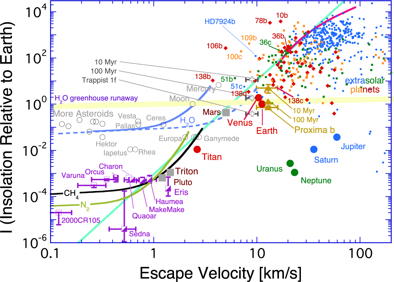
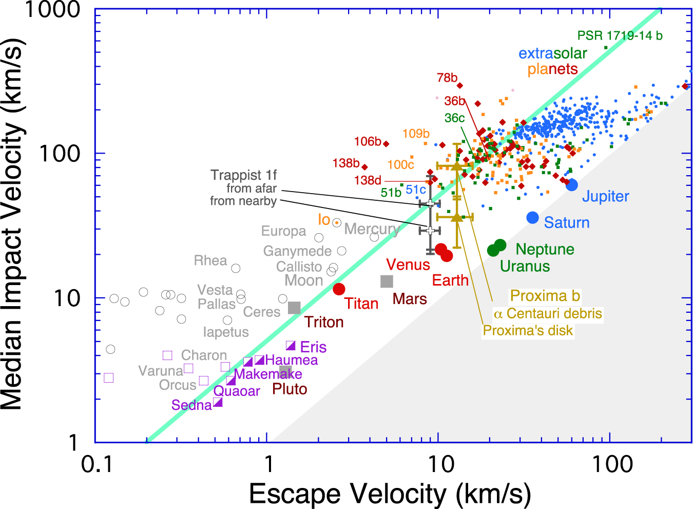
Figure 9. Stabilizing effect of a ballast gas. Here we compare "Europas" of different sizes, one set with only water vapor (m = 18) and the other with the addition of 1 bar of N2 (m = 28). The left-hand panel shows ocean loss times, and the right-hand panel shows the surface temperatures.
Download figure:
Standard image High-resolution image
C.5. Discussion
The uncertainty in evaporation lifetimes of small icy worlds is asymmetric. It is unlikely that our coldest model is too cold. That is, it is unlikely that the true experience could be much more optimistic for continuous habitability than our most long-lived models. But it is entirely possible that our hottest model falls well short of the true escape rate, especially in the presence of a more active Sun. This is only partly because of temperature. The greater uncertainty is photochemistry, which can reduce the mean molecular mass m by a factor of three or more, to the detriment of an alternative Europa as an abode of life.