Abstract
We present a combined observational and theoretical analysis to investigate the nature of plasma turbulence at kinetic scales in the Earth's magnetosheath. In the first decade of the kinetic range, just below the ion gyroscale, the turbulence was found to be similar to that in the upstream solar wind: predominantly anisotropic, low-frequency and kinetic Alfvén in nature. A key difference, however, is that the magnetosheath ions are typically much hotter than the electrons,  , which, together with
  , leads to a change in behavior in the second decade, close to electron scales. The turbulence here is characterized by an increased magnetic compressibility, following a mode we term the inertial kinetic Alfvén wave, and a steeper spectrum of magnetic fluctuations, consistent with the prediction
  that we obtain from a set of nonlinear equations. This regime of plasma turbulence may also be relevant for other astrophysical environments with
  , such as the solar corona, hot accretion flows, and regions downstream of collisionless shocks.
Export citation and abstract BibTeX RIS

Original content from this work may be used under the terms of the Creative Commons Attribution 3.0 licence. Any further distribution of this work must maintain attribution to the author(s) and the title of the work, journal citation and DOI.
1. Introduction
Plasma turbulence is widespread, occurring in a variety of astrophysical environments, such as galaxy clusters, the interstellar medium, and stellar winds. It can be modeled as a cascade of energy from large scales, where the energy is injected, to small, kinetic scales (comparable to the ion and electron gyroscales), where it is thought to be dissipated. However, many aspects of how the cascade operates (in particular at kinetic scales), remain to be understood.
The majority of observations of turbulence at kinetic scales are from the solar wind upstream of the Earth's bow shock (e.g., Alexandrova et al. 2013; Bruno & Carbone 2013; Goldstein et al. 2015; Chen 2016). At scales smaller than the ion gyroscale, the energy spectrum of solar wind density and magnetic fluctuations is observed to be a power law in wavenumber, close to  , down to electron scales (e.g., Alexandrova et al. 2009; Kiyani et al. 2009; Chen et al. 2010a, 2012; Sahraoui et al. 2013). Between the ion and electron scales, the fluctuations are anisotropic, with stronger gradients perpendicular to the mean magnetic field rather than parallel,
  (Chen et al. 2010a), and the amplitude of the density fluctuations relative to the magnetic fluctuations indicates that the turbulence is predominantly low frequency, with a polarization consistent with that of the kinetic Alfvén wave (Boldyrev et al. 2013; Chen et al. 2013b). These features can be interpreted as a cascade of kinetic Alfvén turbulence from ion to electron scales (Howes et al. 2008; Schekochihin et al. 2009; Chen et al. 2010b; Boldyrev & Perez 2012).
When the critical balance principle (Goldreich & Sridhar 1995) is assumed, in which the linear and nonlinear terms of the dynamical equations are comparable, dimensional arguments lead to a perpendicular energy spectrum  , along with an anisotropy
  (Cho & Lazarian 2004; Schekochihin et al. 2009). If the cascade is also assumed to accumulate into intermittent 2D structures, these scalings become
  and
and  (Boldyrev & Perez 2012). The critical balance principle suggests that the linear physics is relevant, even in a strongly turbulent, intermittent cascade. This is borne out in the solar wind, with a variety of observations showing that the fluctuations follow linear relationships to order unity (e.g., Bale et al. 2005; Sahraoui et al. 2009; Howes & Quataert 2010; He et al. 2011; Podesta & Gary 2011; Yao et al. 2011a; Howes et al. 2012; Klein et al. 2012; TenBarge et al. 2012; Chen et al. 2013b, 2013c; Kiyani et al. 2013; Bruno & Telloni 2015; Telloni et al. 2015; Verscharen et al. 2017), and similarly in numerical simulations (e.g., Howes et al. 2011; Boldyrev & Perez 2012; TenBarge & Howes 2012; Verscharen et al. 2012; Franci et al. 2015; Told et al. 2015; Cerri et al. 2016), although there can also be quantitative differences introduced by the nonlinearites (e.g., Boldyrev et al. 2011, 2012; Chen et al. 2013a, 2013b).
The Earth's magnetosheath, the region of solar wind downstream of the bow shock, presents a different environment in which kinetic scale turbulence can be measured, although it has been less comprehensively studied here. This is partly because there are often additional processes taking place which complicate the picture, e.g., instability-generated waves (such as mirror modes, ion cyclotron waves, and whistler waves) and various other non-turbulent structures (see, e.g., Lucek et al. 2005, for a review). However, with careful data selection, these can be avoided, allowing the pure turbulent cascade to be investigated. It has been shown that at ion scales, the magnetic field spectrum in the magnetosheath steepens (e.g., Dudok de Wit & Krasnosel'skikh 1996; Czaykowska et al. 2001; Alexandrova et al. 2008; Chaston et al. 2008; Yordanova et al. 2008; Yao et al. 2011b; Huang et al. 2014; Stawarz et al. 2016; Matteini et al. 2017), the electric field spectrum flattens (Chaston et al. 2008; Stawarz et al. 2016; Matteini et al. 2017), and the turbulence in the kinetic range is intermittent (Dudok de Wit & Krasnosel'skikh 1996; Sundkvist et al. 2007; Stawarz et al. 2016; Vörös et al. 2016) and anisotropic, with  (Mangeney et al. 2006; Alexandrova et al. 2008; Stawarz et al. 2016). These features are similar to the upstream solar wind, which might suggest that a similar type of turbulence is present.
An important difference between the magnetosheath and the upstream solar wind, however, is the ratio of ion and electron temperatures. In the upstream solar wind, the temperatures are typically comparable,  , whereas in the magnetosheath, the ions are typically much hotter,
  (Wang et al. 2012), as a result of processing by the bow shock (e.g., Burgess & Scholer 2013; Krasnoselskikh et al. 2013; Vink et al. 2015). We have found that this can lead to a change in the behavior of the turbulence near electron scales. In this paper, we present the identification of this turbulence regime in measurements from the Magnetospheric Multiscale (MMS) spacecraft, together with a theoretical framework through which it can be understood.
2. Observations
2.1. Data Interval
The observational analysis is based on data from the four MMS spacecraft (Burch et al. 2016) during a period in the Earth's magnetosheath (2015 October 16, 09:24:11–09:25:24) for which burst mode data are available. During this time, the spacecraft were located 11.9 RE from Earth, close to the dusk side magnetopause, with an inter-spacecraft separation of ∼14 km. This period does not contain large-amplitude variations in the magnetic field magnitude (associated with mirror modes) or high-frequency wave packets at electron scales (thought to be whistler waves), allowing the pure turbulent cascade to be studied.
For the magnetic field  , data from the FGM (Fluxgate Magnetometer, Russell et al. 2016) and SCM (Search-Coil Magnetometer, Le Contel et al. 2016) instruments were combined using a wavelet technique (Chen et al. 2010a) to produce 8192 samples s–1 data containing the full range of frequencies (with the crossover between instruments at ∼8 Hz). The electric field
  was measured by the SDP (Spin-Plane Double Probe, Lindqvist et al. 2016) and ADP (Axial Double Probe, Ergun et al. 2016) instruments at the same resolution. FPI (Fast Plasma Investigation, Pollock et al. 2016) was used for the ion and electron densities ni and ne, velocities
  and
and  , and temperatures Ti and Te; the resolution of these moments is 150 ms for the ions and 30 ms for the electrons. A time series of the data from MMS3 for this interval is shown in Figure 1. The average plasma conditions were:
  nT,
nT, 
 ,
,  , with temperature anisotropies
  and
and  . These parameters result in average ion and electron plasma betas
  and
and  (where
  ).
).

Figure 1. Time series of the magnetic field ( ) components in geocentric solar ecliptic (GSE) coordinates (blue, orange, yellow) and magnitude (black), electron number density (ne), electron velocity (
 ) components in GSE (blue, orange, yellow) and magnitude (black), and temperatures
  (blue),
  (orange),
  (yellow) and
  (purple) from MMS3.
Download figure:
Standard image High-resolution imageFrom the magnitude of the ion and electron betas,  , it can be seen that for the ions, the gyroradius
  (where
  is the thermal speed,
  is the gyrofrequency, mi is the mass, and qi is the charge) and inertial length
  (where
  is the Alfvén speed and ρ is the mass density) are similar
  , whereas for the electrons, the gyroradius is much smaller,
  . This results in two sub-ranges between the ion and electron gyroscales: one above the electron inertial scale,
  , and one below,
  . The following sections describe the nature of the fluctuations in each of these ranges.
2.2. Nature of Fluctuations at 

To determine the nature of the fluctuations, first the anisotropy was measured, using the multi-spacecraft technique described by Chen et al. (2010a). Two-point structure functions  were calculated from the time-lagged magnetic field measurements between pairs of spacecraft. The technique mixes spatial and temporal measurements, and assumes the Taylor hypothesis (Taylor 1938) to be satisfied (i.e., that the measured temporal variations correspond to spatial variations in the plasma frame), which appears to be the case, despite the low flow speed and dispersive regime (see Section 2.4). Figure 2 shows
  , binned and averaged as a function of length scale parallel and perpendicular to the local mean field. The range of scales covered is
  , or equivalently
  . It can be seen that the contours of
  are elongated in the parallel direction, and that the value of
  at a scale of 15 km is ∼10 times larger in the perpendicular direction than in the parallel direction. This indicates strongly anisotropic fluctuations
  , consistent with previous findings for magnetosheath (Mangeney et al. 2006; Alexandrova et al. 2008) and solar wind (Chen et al. 2010a) turbulence in the kinetic range.

Figure 2. Magnetic fluctuation energy  as a function of length scale parallel
  and perpendicular
  to the local mean field. Contours are elongated in the
  direction, indicating anisotropic fluctuations
  .
.
Download figure:
Standard image High-resolution imageThe two possible modes in this regime for an isotropic Maxwellian plasma are the kinetic Alfvén wave,

and the oblique whistler wave,

To distinguish these, the correlation between  and
and  can be used, which is negative for the kinetic Alfvén wave and positive for the whistler wave. Figure 3 shows the magnitude-squared wavelet coherence, γ, between
  and
and  , and the phase lag ϕ (black arrows) for
  , measured by MMS3. To avoid complications with the definition of
  was used as a proxy for
  , which requires
  , a condition well-satisfied here. For spacecraft-frame frequencies
  , corresponding to
  and there is a strong anti-correlation. The average phase lag in this range is
  (where the uncertainty is the standard deviation). For
  , the anti-correlation is lost due to noise in the density measurement. This strong anti-correlation, along with the
  anisotropy, indicates the predominantly kinetic Alfvén nature of the turbulence in the first decade of the kinetic range.

Figure 3. Wavelet magnitude-squared coherence γ and phase ϕ (angle of black arrows from the  direction) between
  and
and  . The white dashed line marks the cone of influence. Strong anti-correlation can be seen at spacecraft-frame frequencies
  .
.
Download figure:
Standard image High-resolution imageFigure 4 shows the spectra of various quantities measured by MMS3, calculated using the multitaper method (Percival & Walden 1993). In the range  , the trace magnetic fluctuation spectrum has a power-law index of −2.8 before steepening at electron scales, similar to solar wind observations (e.g., Alexandrova et al. 2009; Kiyani et al. 2009; Chen et al. 2010a, 2012; Sahraoui et al. 2013) and kinetic Alfvén turbulence simulations (e.g., Howes et al. 2011; Boldyrev & Perez 2012), and not far from the
  prediction for intermittent kinetic Alfvén turbulence (Boldyrev & Perez 2012). The trace electric field spectrum, Lorentz transformed into the zero mean velocity frame (Chen et al. 2011), has a spectral index of −0.8, a factor of k2 shallower than the magnetic spectrum, before also steepening at electron scales. The ratio
  is around unity for
  then displays linear scaling for
  , as also seen by Matteini et al. (2017). This is because kinetic Alfvén fluctuations, although electromagnetic in nature, have a significant potential component of the electric field; the ion motion satisfies
  , so the density adjusts to the electric potential as
  , and since
  , the electric field is given by
  . The electron velocity spectral index is −0.9, close to k2 shallower than the magnetic field and similar to the electric field, since the electron velocity is dominated by the
  drift. The ion velocity spectrum, however, is much steeper, similar to in the upstream solar wind (Šafránková et al. 2013, 2016), reaching the instrumental noise around
  . This is because the ions no longer participate in the same
  drift as the electrons, since their gyroradius is much larger than the scales of the electric field fluctuations in this range. Figure 4(d) shows the normalized ratio of density and magnetic fluctuations,
which is  , confirming that the turbulence is predominantly low frequency,
  , and kinetic Alfvén rather than whistler (Boldyrev et al. 2013; Chen et al. 2013b). The increase in
  for
for  is not physical, but due to the density spectrum reaching the noise level.
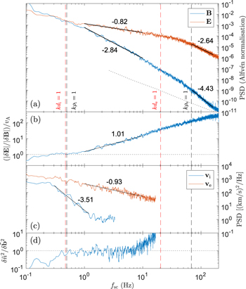
Figure 4. (a) Magnetic field,  , and electric field,
  , power spectra. (b) Ratio of electric and magnetic fluctuations. (c) Ion velocity,
  , and electron velocity,
  , power spectra. (d) Ratio of density and magnetic fluctuations (Equation (3)). The dashed lines mark the plasma microscales under the Taylor hypothesis; the dotted line is the normalized SCM noise floor (Le Contel et al. 2016).
Download figure:
Standard image High-resolution image2.3. Nature of Fluctuations at

While the first decade of the magnetosheath kinetic range,  , described in Section 2.2, is similar to that in the upstream solar wind, the nature of the turbulence changes in the second decade. The kinetic Alfvén wave (Equation (1)) is derived assuming
  ; however, it can be seen that (for
  ) this breaks down at the scale

about halfway between  and
and  for the measured parameters. In the range
  , the kinetic Alfvén wave transforms into a mode with dispersion relation

which we call the inertial kinetic Alfvén wave (see Appendix A for the derivation). This should be distinguished from the standard inertial Alfvén wave derived under the conditions  and
and  (e.g., Lysak & Lotko 1996), which are not satisfied here. Note also that the term "inertial kinetic Alfvén wave" has occasionally been applied to the standard inertial Alfvén wave (Shukla et al. 2009; Agarwal et al. 2011), although the conditions assumed in these works are essentially the same as in Lysak & Lotko (1996) and different from those leading to Equation (5).
The key observational feature of the transition to inertial kinetic Alfvén turbulence is the magnetic compressibility,

For  , and for
  , i.e., in general, the magnetic compressibility increases as energy cascades through
  . This is because for
  , the ion pressure reduces plasma compressibility, which due to pressure balance causes a
  -dependent reduction in
  . For
. For  , however, the compressibility caused by the electron polarization drift becomes stronger than the compressibility due to the
  drift, leading to
  .
.
Figure 5 shows the spectra of  and
and  , and the ratio of these, as measured by MMS3. As for Section 2.2,
  was used as a proxy for
  , and
, and  . It can be seen that at
  , the magnetic compressibility is
  , then this increases through
  , becoming
  by the time
  is reached. In fact, the red line shows the measured compressibility to be following Equation (6) over the whole range between the ion and electron gyroscales. Note that the increase in compressibility is not due to noise; random fluctuations would produce equal power in all three components, resulting in
  (which occurs only for
  , where the noise level is reached). It is also not due to parallel propagating whistler wave packets, which would appear as enhancements in the spectrum with a strong circular polarization (Matteini et al. 2017), but are not present in this interval. The observed magnetic compressibility, therefore, is consistent with a transition to inertial kinetic Alfvén turbulence for
  .
.

Figure 5. Power spectra of  and
and  and magnetic compressibility
  . In the lower panel, the black dotted lines show the asymptotic predictions
  and 1, and the red solid line is Equation (6). The vertical dashed lines are the same as in Figure 4; the additional green line is the transition scale (Equation (4)).
Download figure:
Standard image High-resolution image2.4. Validity of the Taylor Hypothesis
The use of the Taylor hypothesis to interpret Figures 2–5 in the spatial domain requires careful consideration. This assumes that the plasma-frame frequencies are small compared to the frequency of the convected spatial variations  . If the fluctuations follow the kinetic Alfvén wave (Equation (1)) and inertial kinetic Alfvén wave (Equation (5)) dispersion relations, which the measurements of Sections 2.2 and 2.3 are consistent with, this condition (for
  ) becomes
  (see also Howes et al. 2014). For
  , this reduces to
  . Due to the anisotropy
  , this can be well-satisfied, even for
  . For
. For  this reduces to
  , which can be written
  . Therefore, as long as
  does not grow faster than
  (theoretical considerations suggest it actually grows more slowly; see Section 3.2), the Taylor condition would remain valid down to
  .
.
A recent numerical study (Klein et al. 2014) concluded that the Taylor hypothesis is indeed satisfied for kinetic Alfvén turbulence at  and if it was violated significantly shallower spectra would result. The fact that the spectra in Figure 4 match those in the solar wind, as well as expectations from simulations and theory, is consistent with the interpretation that the measured fluctuations are spatial. As a more direct test, Figure 6 shows the normalized magnetic fluctuation amplitudes, as calculated from the second-order structure function, from both the single-spacecraft method (converting from the temporal to spatial domain assuming the Taylor hypothesis) and as direct spatial measurements from the six pairs of MMS spacecraft. There is some scatter in the multi-spacecraft measurements, due to the spacecraft separation vectors being at different angles to the mean field direction, but the average value of
  is similar to the single-spacecraft value of
  , consistent with the Taylor hypothesis being valid down to
  .
.

Figure 6. Normalized magnetic fluctuation amplitude  as a function of scale l measured with the single-spacecraft method assuming the Taylor hypothesis (black line), and with pairs of spacecraft (i, j) as a direct spatial measurement. The vertical dashed lines are the same as in Figure 4.
Download figure:
Standard image High-resolution image
3. Theoretical Model
3.1. Dynamical Equations for Inertial Kinetic Alfvén Turbulence
To understand the nonlinear properties of the cascade, we first derive the dynamical equations for inertial kinetic Alfvén turbulence. We consider strongly anisotropic ( ) fluctuations, and use the ordering
  .
.
The starting equations are the electron continuity and momentum equations. In the electron continuity equation,

the parallel electron velocity can be expressed through the parallel electron current,  , which can, in turn, be expressed through the z component of the magnetic vector potential,
  , as
, as  . Here, e is the magnitude of the electron charge. Due to the small amplitude of the magnetic fluctuations,
  , the deviation of the magnetic field lines from the z direction (large-scale mean field) is small, so the parallel components of the vector fields can be approximated by their z components. This is, however, not true for the parallel gradients, since
  , which are given by

The perpendicular electron velocity is more complicated. It has two parts, the  drift and the polarization drift,

In this expression,  is the
  drift velocity, the convective derivative is
  , and we note that
  . The second term on the right-hand side of Equation (9) is smaller than the first by
  ; however, it needs to be retained since in the continuity equation the leading contribution from the first term cancels out. The electric field has both potential and non-potential components,
  . The non-potential component is small compared to the potential one as it includes the (small) time derivative of the (small) magnetic fluctuations,

although it also needs to be retained for the same reason. The fluctuations of the perpendicular magnetic field component are given by the z component of the magnetic vector potential,  .
.
Substituting these expressions into Equation (7), and keeping the leading order terms, we obtain
We now turn to the electron momentum equation. The parallel component of the equation is

Here, we have made use of  and
and  . The latter condition can be checked a posteriori from the expressions for the parallel and perpendicular velocity components. The electric field is expressed through the scalar and vector potentials,

As can be checked, the electron pressure fluctuations can be neglected compared to the electric potential fluctuations, ϕ, for  . We then get the equation for the z component of the magnetic potential ψ,

To close Equations (11) and (14), we need to find two additional relations among the fluctuating fields. One of these can be found from the perpendicular component of the electron momentum equation. Neglecting the small electron pressure, the force balance in the perpendicular direction is

Writing the perpendicular velocity as  , the electric field is then given by

Since, as we will see later,  , the first term on the right-hand side of Equation (16) is small. Using
  , the relation between the electric potential and the z component of the fluctuating magnetic field is obtained,

For the second relation, we use the fact that kinetic Alfvén fluctuations exist for  . In this case, the ion (and, by quasineutrality, electron) density fluctuations adjust to the electric potential according to the Boltzmann formula,

It can be seen that Equations (17) and (18) agree with the force balance in the single-fluid momentum equation,  . We can now eliminate the
  and ϕ fluctuations from Equations (11) and (14) in favor of the density fluctuations. Using the dimensionless variables
  ,
,  ,
,  ,
,  , and omitting the prime signs, we obtain the nonlinear system of equations for inertial kinetic Alfvén turbulence:

The nonlinearities in these equations appear in the second terms on the left-hand sides, and in the parallel gradients on the right-hand sides,

Without the nonlinear terms, these equations reproduce the inertial kinetic Alfvén wave dispersion relation (Equation (36)), and the relation between  and ψ for these modes,

The last equation agrees with Equation (6) since  represents the perpendicular magnetic fluctuations, and
  in the above normalization.
3.2. Energy Spectrum and Anisotropy
From Equations (19) and (20), we can derive the spectrum of inertial kinetic Alfvén turbulence. In the absence of energy supply and dissipation, the equations conserve the energy
In a turbulent state, both terms of E are of the same order. For scales  , this means that
  , where
  and
and  denote the typical fluctuations of the fields at the scale λ across the background magnetic field. In the same limit, the nonlinearity is dominated by the terms on the left-hand sides of Equations (19) and (20), and the nonlinear time can be estimated as
  . Assuming a constant energy flux through scales,
  , leads to the scaling of the density and magnetic fluctuations
  . Applying the Fourier transform in the plane perpendicular to the background magnetic field, the spectrum of density and perpendicular fluctuations is obtained,
  . In the data interval discussed in Section 2, the scaling range between
  and
and  is not large (a factor of 3.4), so a well-developed power-law spectrum is not present, but the measured spectral index can still be compared to the prediction in the limited range. Figure 5 shows the spectral index to be −3.6 for the
  fluctuations between
  and
and  , which is not far from the predicted value of
  .
.
The anisotropy implied by the critical balance condition can also be determined. Balancing the linear and nonlinear terms in Equations (19) and (20),  , we obtain the relation between the parallel and perpendicular scales
  . In Fourier space this means that the turbulent energy is concentrated in the region
  , which becomes progressively broader in
  and less anisotropic as
  increases. This suggests, therefore, that in contrast to standard Alfvén and kinetic Alfvén turbulence, the energy cascade in inertial kinetic Alfvén turbulence supplies energy more efficiently to
  rather than
  modes. This anisotropy also implies that the Taylor condition becomes better satisfied as
  increases (see Section 2.4). The current data interval does not allow the scale-dependence of the anisotropy to be tested, but this could be done in future studies with larger data sets, and also tested in numerical simulations.
3.3. Inertial Whistler Turbulence
The condition derived in Section 3.2 that critically balanced inertial kinetic Alfvén turbulence becomes more isotropic toward smaller scales leads to the interesting possibility that the cascade may transition to inertial whistler turbulence if the anisotropy reduces sufficiently. This is because there is a maximum value of  at which inertial kinetic Alfvén waves can exist (see Appendix A); the broadening of the spectrum in the
  direction would lead to the turbulence reaching
  , which is the whistler frequency range.
For completeness, we give here the dynamical equations for inertial whistler turbulence. The basic Equations (11) and (14) hold for whistler turbulence as well; however, the additional condition (18) needs to be modified. Due to the high frequency of the whistlers, the density fluctuations do not follow the electric potential and remain small,

We can thus neglect the density fluctuations in Equations (11) and (14), and use Equation (17) to remove the electric potential fluctuations. Using again the normalized variables, and also  , with the primes omitted, we obtain the nonlinear equations for inertial whistler turbulence:

Linearization of these equations leads to the inertial whistler wave dispersion relation, which (in unnormalized variables) is given by

and is also derived in Appendix B.
Due to the structural similarity of the inertial kinetic Alfvén and inertial whistler equations, (19), (20) and (25), (26), the spectrum of magnetic fluctuations in inertial whistler turbulence is the same as that derived in Section 3.2, with the difference that the transition to the inertial regime occurs at  rather than
  . This spectrum for inertial whistler turbulence has also been discussed previously (Biskamp et al. 1996, 1999; Meyrand & Galtier 2010; Andrés et al. 2014). The structural similarity between the equations means that the anisotropy implied by the critical balance condition (discussed in Section 3.2) is also the same, meaning that the increasing isotropization would continue if the inertial kinetic Alfvén cascade transitions to inertial whistler turbulence.
The main physical difference between inertial kinetic Alfvén and inertial whistler turbulence is the ion dynamics, as discussed above, which leads to negligibly small density fluctuations in inertial whistler turbulence (see Appendix B). The magnetic compressibility, however, is the same, with  for both types of turbulence at sub-electron-inertial scales. The measurements in Figure 5, therefore, allow for the possibility of a transition to inertial whistler turbulence between
  and
and  . Further measurements will be required to determine whether, and under what conditions, such a transition occurs.
4. Discussion
We have presented measurements of kinetic scale turbulence in the Earth's magnetosheath, which have the conditions  and
and  . In the first decade of the kinetic range, the turbulence is similar to that in the upstream solar wind: it is predominantly low-frequency (
 ), anisotropic (
 ), and kinetic Alfvén in nature, with spectra that match theoretical predictions and numerical simulations. In the second decade, however, a regime of inertial kinetic Alfvén turbulence has been identified by the increase in magnetic compressibility following that of the inertial kinetic Alfvén wave (Equation (6)). A set of nonlinear equations (Equations (19)–(20)) has been derived, which can be used to obtain the spectrum of magnetic fluctuations,
  , between the electron inertial scale and electron gyroscale, which is consistent with the observed spectral steepening. Interestingly, this turbulence is expected to exhibit a qualitatively different scale-dependent anisotropy to standard Alfvén and kinetic Alfvén turbulence, becoming less anisotropic toward smaller scales. This increasing isotropization may lead to a transition to inertial whistler turbulence (described by Equations (25) and (26)) if the frequency reaches
  . We plan to investigate these aspects with further observations and numerical simulations.
As well as in the Earth's magnetosheath, inertial kinetic Alfvén turbulence may also be present in several other astrophysical environments, with comparable plasma parameters. For example, the fast solar wind model of Chandran et al. (2011) predicts  and
and  at 10 solar radii from the Sun, a regime in which inertial kinetic Alfvén turbulence would be expected to constitute a significant fraction of the kinetic range. This region of the solar corona will soon be measured in situ by the Solar Probe Plus spacecraft (Fox et al. 2016), allowing this to be tested directly. Similarly, in hot accretion flows, where turbulent heating is thought to be important, the ions are likely to be hotter than the electrons (Quataert 1998), allowing the possibility of inertial kinetic Alfvén turbulence at small scales. Finally, collisionless shocks, such as the one that generates the Earth's magnetosheath, are common throughout the universe, leading to turbulent regions of space with large
  (Treumann 2009; Ghavamian et al. 2013). Inertial kinetic Alfvén turbulence, therefore, may be quite widespread, and a possible route through which astrophysical plasmas are heated.
C.H.K.C. is supported by an STFC Ernest Rutherford Fellowship. S.B. is supported by the Space Science Institute, NSF grant AGS-1261659, and by the Vilas Associates Award from UW Madison. We acknowledge the MMS team for producing the data, which were obtained from the MMS Science Data Center (https://lasp.colorado.edu/mms/sdc/).
Appendix A: Derivation of the Inertial Kinetic Alfvén Wave
In a  plasma, when the wave propagation is oblique,
  , the Alfvén wave transforms into the kinetic Alfvén wave for scales
  . The situation is different, however, when either
  or
or  is small. In the regime of extremely small electron plasma beta
  , and
, and  , the Alfvén wave transforms into the inertial Alfvén wave (e.g., Lysak & Lotko 1996). In this case, the electron thermal velocity is much smaller than the Alfvén velocity, and the electrons do not adjust instantaneously to the electric field acting along the magnetic field lines. The regime here, however, is different,
  , and the standard inertial Alfvén theory does not apply.
The dispersion relation for the standard kinetic Alfvén wave (e.g., Howes et al. 2006), derived under the assumption  , is
, is

where  has been assumed in the last expression. Note that in the linear theory, the global and local mean magnetic field directions are the same, and here we use z for this direction. It can be seen, however, that the frequency of the kinetic Alfvén wave becomes larger than
  for
for

For  and
and  , this happens at a scale much larger than the electron gyroscale.
In the frequency range  , the kinetic Alfvén wave transforms into the inertial kinetic Alfvén wave. To derive this mode, we consider a collisionless plasma with
  , at sub-ion scales
  . The wave modes can be found from the equation
  , where
  is the plasma dielectric tensor, and Ej is the electric field. Under the additional assumption
  , the components of the tensor Dij take the form


where the wave vector has components  .
.
The dispersion relation for the inertial kinetic Alfvén wave obtained from this equation is

When the electron inertial corrections are small,  , this is similar to the dispersion relation of the standard kinetic Alfvén wave (Equation (28)), although in a different phase space region,
  , which indicates that the dispersion relation is not sensitive to ω/(kzvth,e). In the opposite case,
  , the inertial kinetic Alfvén wave frequency becomes

A similar derivation for the Alfvén modes at low β can also be made starting from the gyrokinetic description (e.g., Howes et al. 2006; Zocco & Schekochihin 2011).
The inertial kinetic Alfvén wave exists for  , which, together with the dispersion relation (Equation (36)), allows the required obliquity to be determined. At
  the wave requires
  , and at
  the condition is
  .
.
The density fluctuations associated with the inertial kinetic Alfvén wave are
and they are anti-correlated with the fluctuations of the magnetic field strength,

From Equations (38) and (39), the expression for the magnetic compressibility is obtained,

Appendix B: Derivation of the Inertial Whistler Wave
The whistler wave, unlike the kinetic Alfvén wave, exists for frequencies  and transforms into the inertial whistler wave at
  . It can be derived from the same Equations (30)–(35), if Dxx is replaced by

The dispersion relation for the inertial whistler wave is then obtained,

Without the electron inertial corrections,  , the wave exists only for
  , where we recover the well-known whistler dispersion relation. In the opposite limit,
  , the whistlers exist for
  , so the second term in the square bracket in Equation (42) can always be neglected. Equation (42) then matches the previously studied whistler wave in the inertial regime (e.g., Biskamp et al. 1996, 1999).
The density fluctuations associated with the inertial whistler wave are given by
and are positively correlated with the fluctuations of the magnetic field strength,

For  , the wave satisfies
  and we recover the well-known relation,
  . In the inertial regime
  it satisfies
  , and we obtain
  . In both cases, the density fluctuations are much smaller than the magnetic fluctuations. Also, in both cases the magnetic compressibility is given by