


ABSTRACT
We present the first results of the Gould's Belt Distances Survey (GOBELINS), a project aimed at measuring the proper motion and trigonometric parallax of a large sample of young stars in nearby regions using multi-epoch Very Long Baseline Array (VLBA) radio observations. Enough VLBA detections have now been obtained for 16 stellar systems in Ophiuchus to derive their parallax and proper motion. This leads to distance determinations for individual stars with an accuracy of 0.3 to a few percent. In addition, the orbits of six multiple systems were modelled by combining absolute positions with VLBA (and, in some cases, near-infrared) angular separations. Twelve stellar systems are located in the dark cloud Lynds 1688; the individual distances for this sample are highly consistent with one another and yield a mean parallax for Lynds 1688 of  mas, corresponding to a distance
  pc. This represents an accuracy greater than 1%. Three systems for which astrometric elements could be measured are located in the eastern streamer (Lynds 1689) and yield an estimate of
  mas, corresponding to a distance
  pc. This suggests that the eastern streamer is located about 10 pc farther than the core, but this conclusion needs to be confirmed by observations of additional sources in the eastern streamer (currently being collected). From the measured proper motions, we estimate the one-dimensional velocity dispersion in Lynds 1688 to be 2.8 ± 1.8 and 3.0 ± 2.0 km s−1, in R.A. and decl., respectively; these are larger than, but still consistent within
  of, those found in other studies.
Export citation and abstract BibTeX RIS
1. INTRODUCTION
1.1. The Gould's Belt
The Gould's Belt (see Poppel 1997 for a comprehensive review) is a local Galactic structure containing much of the dense interstellar matter and many of the young stars within a few hundred parsecs of the Sun. It was originally identified by John Herschel (circa 1847) and Benjamin Gould (in the 1870s), who noticed that most of the brightest stars were neither randomly distributed in the sky nor associated with the Galactic plane, but instead concentrated along a great circle tilted by about 18° from the Galactic equator. Modern studies (e.g., Perrot & Grenier 2003) have shown that the Gould's Belt is a broad elliptical ring of young stars and interstellar matter with semimajor and semiminor axes of 375 pc and 235 pc, respectively. The center of the structure is located at about 105 pc from the Sun, in the direction of the Galactic anti-center. There is ample evidence that the Gould's Belt is expanding and has a dynamical age of order 30 Myr; Perrot & Grenier (2003) indicate 26.4 ± 0.4 Myr. The oldest stars associated with the Gould's Belt are also about 30 Myr old (e.g., Stothers & Frogel 1974), but T Tauri stars (age 106–107 years) as well as protostars (≲105 years) and pre-stellar cores are also present, showing that star formation is still ongoing.
The Gould's Belt contains several million solar masses of interstellar material and includes all the nearby sites of active star formation (Orion, Ophiuchus, Perseus, etc.). These have been the benchmarks against which theories of star formation have been tested. Indeed, numerous "Gould's Belt surveys" targeting these regions have been carried out over the years—for instance, the James Clerk Maxwell Telescope Legacy Survey of Nearby Star-forming Regions in the Gould Belt (Ward-Thompson et al. 2007), the Spitzer Gould Belt (Dunham et al. 2015) and c2d (Evans et al. 2009) Legacy Surveys, and the Herschel Gould's Belt Survey (André et al. 2010). To take full advantage of this wealth of high quality information, it is fundamental to have accurate distance measurements to each of the regions in the Gould's Belt. In addition, these regions are a few hundred parsecs away and typically a few tens of parsecs across—and therefore presumably also a few tens of parsecs deep. As a consequence, using a single mean distance (however accurately measured) for all young stellar objects (YSOs) in a given region will result in typical distance errors in excess of 10% for the individual YSOs. A case in point is that of the Taurus star-forming region, which is located at a mean distance of about 145 pc, but is about 30 pc deep (Loinard et al. 2007; Torres et al. 2007, 2009, 2012). Using the mean distance to Taurus to calculate luminosities for YSOs located on the near side of the complex (at 130 pc) results in an error of 25%. Thus it is not sufficient to have an accurate mean distance for each region. Rather, it is highly desirable to have accurate distances to a substantial sample of individual objects within each region. Such detailed information also makes it possible to reconstruct the internal three-dimensional (3D) structure of the clouds.
Recently, Bouy & Alves (2015) used stars from the Hipparcos catalogue to determine the 3D distribution of the spatial density of OB stars within 500 pc from the Sun. They found no evidence for a ring-like structure and claimed that the Gould's Belt is the result of a 2D projection effect. They also proposed that the apparent rotation and expansion of the belt is due to relative motions associated with Galactic dynamics, but this needs to be investigated through accurate measurements of the dynamical state of the Belt.
1.2. VLBI Distance Determinations
Understanding the processes of star formation requires accurate observational constraints. The observational signatures predicted by star formation models have to be compared to actual observations, but a direct comparison can only be performed when the stellar properties, such as source size, luminosity, and mass, are well determined. Frequently the distances to star-forming regions are poorly constrained because they are obscured by molecular gas and dust. In such cases, inaccurate distances are often the main source of error in intrinsic parameter determinations.
Numerous indirect methods can be used to estimate the distance to young stars (e.g., de Grijs 2011), but they typically result in systematic uncertainties in excess of 20%. Only trigonometric parallaxes can provide unbiased distance measurements, but they are notoriously challenging to obtain. For instance, the trigonometric parallax of a star at 200 pc is 5 milli-arcseconds (mas), so an astrometric accuracy of 50 micro-arcseconds (μas) on the parallax would be required to measure that distance to 1% accuracy. This is more than one order of magnitude better than the astrometry delivered by the Hipparcos satellite (Perryman et al. 1997). Indeed, Hipparcos did not significantly improve our knowledge of the distance to star-forming regions in the Gould's Belt (e.g., Bertout et al. 1999). Also, the Hipparcos result on the distance to the Pleiades cluster, which is commonly used for testing theoretical stellar models, disagrees with all distance determinations obtained through other methods (Melis et al. 2014; David et al. 2016). The upcoming Gaia astrometric mission (de Bruijne 2012) will likely reach an accuracy of a few tens of μas, sufficient for percent accuracy determinations of distances in the Gould's Belt. However, since it operates at optical wavelengths, Gaia will be limited to stars that have low extinction. This will be an issue in star-forming regions like Orion, Ophiuchus, or Serpens, where values of AV larger than 10 are common (Cambrésy 1999; Ridge et al. 2006).
For accurate astrometry, an alternative to optical-wavelength space missions is provided by Very Long Baseline Interferometry (VLBI; e.g., Thompson et al. 2007; Reid & Honma 2014). VLBI observations at centimeter wavelengths typically reach an angular resolution of order 1 mas. When VLBI observations are phase-referenced to a bright nearby source, the angular offset between the target and the reference source can be measured to an accuracy of ∼20 to 300 μas, depending on the signal-to-noise ratio of the detection, the declination of the source, and the distance between the target and the reference source (Pradel et al. 2006). The reference sources are usually distant quasars that are very nearly fixed on the celestial sphere. Thus the measured offset between the reference source and the target can be transformed into accurate coordinates for the target. When several such observations collected over 1 year or more are combined, the parallax and proper motion of the target can be measured with high accuracy. Also, the astrometry quality of both VLBI and Gaia observations can be tested by considering objects that both instruments can detect.
Two technical points are worth mentioning here. The first is that a systematic error on the target coordinates will obviously occur if the reference quasar position is not well known. The positional errors of reference calibrators used in VLBI observations are typically between 0.5 and 10 mas, so this is the level of accuracy that can be expected on absolute coordinates derived from VLBI data. However, this additive error will equally affect all observations of a given target (as long as the same calibrator is used), and hence have no measurable effect on the parallax and proper motion measurements obtained from multi-epoch observations. The second, potentially more serious issue is that because of emerging jet components, the photocenter of the quasars may shift with time when accuracies of a few μas on positions and a few μas yr−1 on proper motions are reached (e.g., Reid & Brunthaler 2004). Because our typical positional errors are  , this problem will not be relevant for the data presented here, and can be mitigated by including several reference sources in the observations and monitoring their relative positions as a function of time (e.g., Reid & Honma 2014).
VLBI astrometry can only be applied to a specific class of targets if they are detectable in VLBI observations (e.g., Thompson et al. 2007; Reid & Honma 2014). This requires that the potential targets not only be radio sources but also have an average brightness temperature in excess of ∼106 K within the synthesized beam (i.e., be non-thermal sources), as VLBI arrays do not have sufficient sensitivity to detect weaker emission.17
A summary of the mechanisms that produce non-thermal radio emission in YSOs is provided in Appendix
1.3. GOBELINS
GOBELINS was approved by the Telescope Allocation Committee of the National Radio Astronomy Observatory in the spring of 2010. It followed a two-stage strategy. During the first phase, large maps of each of the regions of interest were obtained, using conventional interferometry observations, with the Karl G. Jansky Very Large Array (VLA; we called this first phase of the project the Gould's Belt Very Large Array Survey). These maps (published by Dzib et al. 2013, 2015; Kounkel et al. 2014; Ortiz-León et al. 2015; and Pech et al. 2016) enabled us to identify radio-bright YSOs in each region and attempt a first separation between thermal and non-thermal sources. For instance, in Ophiuchus, Dzib et al. (2013) identified 56 radio sources associated with YSOs and proposed that for ≳50% of them, the emission is of non-thermal origin. The second stage consists in multi-epoch VLBI observations of the selected targets with the Very Long Baseline Array (VLBA; Napier et al. 1994), to measure the astrometric elements (trigonometric parallax and proper motion) of each target. In this paper, we report on the first VLBI observations of the sources in the Ophiuchus region.
The results from GOBELINS will be used first and foremost to pinpoint the location of the regions of star formation within the Gould's Belt, as well as their internal three-dimensional structure. In addition, since the proper motion of each target will be measured simultaneously with its trigonometric parallax, the transverse component of the velocity vector will be obtained. In many cases, the radial velocity will be available from the literature or could be measured with dedicated optical or near-infrared (NIR) spectroscopy. Thus GOBELINS will also provide the complete velocity vector for many targets. This will enable us to examine both the internal dynamics of each region and the large-scale relative motions of the different clouds in the Gould's Belt (see Rivera et al. 2015 for a preliminary example). In particular, these measurements will help characterize the overall dynamics of the Gould's Belt and will be relevant to the understanding of its very origin.
GOBELINS will also provide radio images of a large sample of YSOs at milli-arcsecond resolution. This is unparalleled at any other wavelength, and will enable us to characterize the population of young, very tight, binary and multiple systems (see Torres et al. 2012 and Dzib et al. 2010 for examples of young multiple systems characterized by VLBI observations), as well as the magnetic structures around young stars (R.M. Torres et al. 2016, in preparation). Finally, these results will enable us to study the physical processes underlying the radio emission. For instance, the Gould's Belt Very Large Array Survey data (Dzib et al. 2013, 2015; Kounkel et al. 2014; Ortiz-León et al. 2015; Pech et al. 2016) have shown that the radio emission from YSOs is reasonably correlated with their X-ray luminosity, following the so-called Güdel-Benz relation (Guedel & Benz 1993; Benz & Guedel 1994). The VLBI observations will enable us to unambiguously separate the thermal and non-thermal components and re-examine this relation in more detail. It will also allow us to examine the prevalence of non-thermal radio emission in young stars as a function of their age and mass, providing clues regarding the magnetic evolution of YSOs.
1.4. The Ophiuchus Region
As mentioned earlier, in the present paper we will focus on the GOBELINS observations of the Ophiuchus region. Ophiuchus is one of the best-studied regions of star formation (see Wilking et al. 2008 for a recent review). It consists of a centrally condensed core associated with the dark cloud Lynds 1688 (where AV = 50 to 100 magnitudes; Wilking et al. 2008) and several filamentary clouds (collectively known as the "streamers") extending toward the east (Lynds 1689 is a particularly prominent dark cloud associated with the eastern streamer) and the northeast (see Figure 1 in this paper and Figure 1 in Dzib et al. 2013).
The distance to Ophiuchus has been discussed in some detail by Wilking et al. (2008), Lombardi et al. (2008), Loinard et al. (2008), and Mamajek (2008). The canonical value of 160 pc (Bertiau 1958; Whittet 1974; Chini 1981) remained in use until very recently. Evidence for a somewhat shorter distance (120–145 pc) started to emerge from optical photometric and astrometric studies of the nearby Upper Scorpius subgroup (de Geus et al. 1989; de Zeeuw et al. 1999). The implications for Ophiuchus itself, however, were limited by the unclear relation between Upper Scorpius and Ophiuchus (see Wilking et al. 2008 for a discussion of this topic). More recently, Mamajek (2008) used the trigonometric parallaxes of the stars illuminating seven reflection nebulae within 5° of the Ophiuchus core to derive an estimate of 135 ± 8 pc. Both Knude & Hog (1998) and Lombardi et al. (2008) combined Hipparcos parallaxes and extinction measurements to conclude that Ophiuchus is at a distance of about 120 pc. Lombardi et al. (2008), in particular, report a mean distance of 120 ± 6 pc for the entire region, with some evidence that the streamers might be ∼10 pc closer than the core. This would be consistent with the distance of 96 ± 9 pc derived by Le Bouquin et al. (2014; see also Schaefer et al. 2008) for the pre-main sequence binary Haro 1–14c, located in the northeastern streamer.
It is important to note that none of the measurements mentioned so far involve direct trigonometric parallaxes to Ophiuchus cluster members. This is, of course, because the stars in that cluster are too deeply embedded to be detectable with Hipparcos or ground-based optical telescopes. Indeed, to date, there are only two published trigonometric parallaxes for Ophiuchus, and both were obtained through VLBI observations. The first measurement was reported by Imai et al. (2007) and targeted water masers associated with the Class 0 protostar IRAS 16293-2422, located in the northern part of Lynds 1689. They derive a distance of  pc, significantly larger than the 120–140 pc estimates that seem to emerge from the previously described recent studies of the Ophiuchus core. It is not clear if this discrepancy stems from issues with one or more of the distance measurements, or if it is indicative that the eastern streamer is significantly more distant than the core. The second parallax measurement was reported by Loinard et al. (2008), and focused on two young stars (DoAr 21 and S1) located toward the Ophiuchus core. They obtain 120 ± 5 pc for the mean distance to these two stars, and adopt this value as the best estimate of the distance to the Ophiuchus core.
In summary, there is a growing consensus that the Ophiuchus core is at 120–140 pc, but reducing the level of uncertainty regarding the distance has proven difficult. In addition, there are some conflicting results regarding the orientation of the streamers relative to the core. This unsatisfactory state of affairs largely results from the scarcity of direct parallax measurements to Ophiuchus members.
In this paper we present new VLBA observations taken over a period of 4 years as part of GOBELINS, and report on the detection of 26 young stellar systems in the Ophiuchus region (corresponding to 34 individual young stars, as some of the systems are multiple). The target sample and observing strategy are described in Section 2, the detections are described in Section 3, and the properties of the detected radio emission are analyzed in Appendix
2. OBSERVATIONS, CORRELATION, AND DATA REDUCTION
The observations were obtained with the National Radio Astronomy Observatory's VLBA at ν = 5 and 8 GHz. We report on a total of 86 projects (code BL175), observed between March 2012 and April 2016, and scheduled either dynamically or on a fixed-date basis. Observations were usually obtained within 3 weeks of the equinoxes (March 21 and September 22) for each year; this corresponds to the maximum elongation of the parallax ellipse. The data were recorded in dual polarization mode with 256 MHz of bandwidth in each polarization, covered by 8 separate 32 MHz intermediate frequency (IF) channels. Projects observed during the first ∼1.5 years of our program were taken at 8 GHz (Table 1). We switched to 5 GHz after the upgrade of the C-band receivers of the VLBA, which resulted in an increase of the bandwidth and sensitivity at that frequency.
Table 1. Observed Epochs
| Project | Observation | Observed Fields Centers | Observed | |
|---|---|---|---|---|
| Code | Date | R.A. ( ) ) |
Decl. ( ) ) |
Band |
| BL175B0 | 2012 Mar 13 | 16 27 55.92 | −24 47 24.82 | X |
| BL175B1 | 2012 Mar 25 | 16 27 30.82 | −24 47 27.21 | X |
| BL175B2 | 2012 Apr 09 | 16 27 24.36 | −24 42 13.39 | X |
| BL175B3 | 2012 Apr 21 | 16 25 49.10 | −24 38 31.00 | X |
| BL175B4 | 2012 Apr 24 | 16 27 15.70 | −24 38 45.68 | X |
| BL175B5 | 2012 Apr 29 | 16 28 04.65 | −24 34 56.66 | X |
| BL175B6 | 2012 May 01 | 16 25 56.80 | −24 30 23.76 | X |
| BL175B7 | 2012 May 05 | 16 26 07.63 | −24 27 41.73 | X |
| BL175B8 | 2012 May 09 | 16 27 32.68 | −24 33 24.54 | X |
| BL175B9 | 2012 May 11 | 16 27 18.17 | −24 28 52.96 | X |
| BL175BA | 2012 May 12 | 16 26 42.44 | −24 26 26.12 | X |
| BL175BB | 2012 Aug 19 | 16 26 03.01 | −24 23 36.42 | X |
| BL175BC | 2012 Sep 01 | 16 27 30.83 | −24 47 27.14 | X |
| BL175C0 | 2012 Sep 03 | 16 36 17.50 | −24 25 55.44 | X |
| BL175BD | 2012 Sep 09 | 16 26 29.67 | −24 19 05.85 | X |
| BL175BE | 2012 Oct 20 | 16 25 49.10 | −24 38 31.00 | X |
| BL175BF | 2012 Oct 30 | 16 27 15.70 | −24 38 45.71 | X |
| BL175BG | 2012 Nov 01 | 16 26 51.70 | −24 14 41.50 | X |
| BL175BH | 2012 Nov 26 | 16 25 56.80 | −24 30 23.76 | X |
| BL175BI | 2012 Nov 28 | 16 26 07.63 | −24 27 41.73 | X |
| BL175BJ | 2012 Nov 30 | 16 27 32.68 | −24 33 24.54 | X |
| BL175BK | 2012 Dec 07 | 16 27 18.17 | −24 28 52.96 | X |
| BL175BL | 2012 Dec 08 | 16 26 42.44 | −24 26 26.12 | X |
| BL175BM | 2012 Dec 09 | 16 26 03.01 | −24 23 36.42 | X |
| BL175BN | 2012 Dec 16 | 16 26 26.01 | −24 23 41.26 | X |
| BL175BO | 2012 Dec 21 | 16 26 29.67 | −24 19 05.85 | X |
| BL175BP | 2012 Dec 28 | 16 27 05.16 | −24 20 07.82 | X |
| BL175ZQ | 2013 Jan 25 | 16 26 49.23 | −24 20 03.35 | X |
| BL175BR | 2013 Feb 01 | 16 26 51.70 | −24 14 41.50 | X |
| BL175BS | 2013 Apr 27 | 16 31 57.16 | −24 56 43.77 | X |
| BL175A9 | 2013 May 01 | 16 27 55.92 | −24 47 24.82 | X |
| BL175BT | 2013 May 21 | 16 31 38.57 | −25 32 20.08 | X |
| BL175BU | 2013 May 29 | 16 31 17.60 | −24 32 02.46 | X |
| BL175BV | 2013 Jun 06 | 16 32 11.80 | −24 40 21.89 | X |
| BL175BW | 2013 Jun 15 | 16 32 45.24 | −24 36 47.42 | X |
| BL175BX | 2013 Jun 23 | 16 30 32.21 | −24 33 17.86 | X |
| BL175AA | 2013 Jun 28 | 16 27 30.82 | −24 47 27.21 | X |
| BL175BY | 2013 Jul 16 | 16 34 21.10 | −23 56 25.19 | X |
| BL175BZ | 2013 Aug 07 | 16 31 40.68 | −24 15 16.49 | X |
| BL175E0 | 2013 Sep 01 | 16 27 30.82 | −24 47 27.21 | C |
| 16 26 16.31 | −24 22 14.00 | |||
| BL175E1 | 2013 Sep 02 | 16 27 18.18 | −24 28 52.99 | C |
| 16 26 42.44 | −24 26 26.27 | |||
| BL175E2 | 2013 Sep 03 | 16 32 11.79 | −24 40 21.92 | C |
| 16 36 17.50 | −24 25 55.41 | |||
| BL175E3 | 2013 Sep 05 | 16 31 38.58 | −25 32 20.08 | C |
| 16 32 45.24 | −24 36 47.33 | |||
| BL175E4 | 2013 Sep 07 | 16 27 32.68 | −24 33 24.54 | X |
| BL175E5 | 2013 Sep 19 | 16 27 20.03 | −24 40 29.53 | C |
| 16 27 22.96 | −24 22 36.60 | |||
| BL175E7 | 2013 Sep 24 | 16 30 32.21 | −24 33 17.86 | C |
| 16 31 17.60 | −24 32 02.46 | |||
| BL175G0 | 2014 Mar 01 | 16 27 30.82 | −24 47 27.21 | C |
| 16 26 16.31 | −24 22 14.00 | |||
| BL175G1 | 2014 Mar 03 | 16 27 18.18 | −24 28 52.99 | C |
| 16 26 42.44 | −24 26 26.27 | |||
| BL175G2 | 2014 Mar 04 | 16 32 11.79 | −24 40 21.92 | C |
| 16 36 17.50 | −24 25 55.41 | |||
| BL175GB | 2014 Mar 05 | 16 26 47.73 | −24 15 37.45 | C |
| BL175G3 | 2014 Mar 06 | 16 31 38.58 | −25 32 20.08 | C |
| 16 32 45.24 | −24 36 47.33 | |||
| BL175G4 | 2014 Mar 09 | 16 27 32.68 | −24 33 24.54 | X |
| BL175G5 | 2014 Mar 10 | 16 27 20.03 | −24 40 29.53 | C |
| 16 27 22.96 | −24 22 36.60 | |||
| BL175G6 | 2014 Mar 13 | 16 27 55.92 | −24 47 24.82 | C |
| 16 28 04.65 | −24 34 56.66 | |||
| BL175G7 | 2014 Mar 14 | 16 30 32.21 | −24 33 17.86 | C |
| 16 31 17.60 | −24 32 02.46 | |||
| BL175G8 | 2014 Mar 24 | 16 31 40.68 | −24 15 16.49 | C |
| 16 31 57.16 | −24 56 43.77 | |||
| BL175G9 | 2014 Mar 25 | 16 34 21.10 | −23 56 25.19 | C |
| 16 25 49.10 | −24 38 31.00 | |||
| BL175GA | 2014 Apr 08 | 16 26 02.22 | −24 29 02.76 | C |
| 16 26 57.20 | −24 20 05.59 | |||
| BL175GC | 2014 Apr 01 | 16 27 19.49 | −24 41 40.74 | C |
| BL175GR | 2014 Jun 05 | 16 26 42.44 | −24 26 26.27 | C |
| 16 27 18.18 | −24 28 52.99 | |||
| BL175DY | 2014 Aug 29 | 16 27 20.03 | −24 40 29.53 | C |
| 16 27 22.96 | −24 22 36.6 | |||
| BL175CR | 2014 Oct 07 | 16 27 30.82 | −24 47 27.21 | C |
| 16 26 16.31 | −24 22 14.00 | |||
| BL175CS | 2014 Oct 12 | 16 27 18.18 | −24 28 52.99 | C |
| 16 26 42.44 | −24 26 26.27 | |||
| BL175CT | 2014 Oct 15 | 16 32 11.79 | −24 40 21.92 | C |
| 16 36 17.50 | −24 25 55.41 | |||
| BL175EX | 2015 Feb 27 | 16 27 30.82 | −24 47 27.21 | C |
| 16 26 16.31 | −24 22 14.00 | |||
| BL175EY | 2015 Mar 02 | 16 27 18.18 | −24 28 52.99 | C |
| 16 26 42.438 | −24 26 26.27 | |||
| BL175EZ | 2015 Mar 20 | 16 32 11.79 | −24 40 21.92 | C |
| 16 36 17.50 | −24 25 55.41 | |||
| BL175F3 | 2015 Mar 15 | 16 27 20.03 | −24 40 29.53 | C |
| 16 27 22.96 | −24 22 36.60 | |||
| BL175F7 | 2015 Apr 29 | 16 26 02.22 | −24 29 02.76 | C |
| 16 26 57.20 | −24 20 05.59 | |||
| BL175FY | 2015 Aug 30 | 16 26 02.22 | −24 29 02.76 | C |
| 16 26 57.20 | −24 20 05.59 | |||
| BL175FZ | 2015 Sep 03 | 16 27 05.16 | −24 20 07.80 | C |
| 16 27 20.03 | −24 40 29.53 | |||
| BL175GS | 2015 Sep 04 | 16 30 35.64 | −24 34 19.00 | C |
| 16 31 20.19 | −24 30 01.06 | |||
| BL175GT | 2015 Sep 15 | 16 27 19.49 | −24 41 40.74 | X |
| BL175GU | 2015 Sep 19 | 16 26 47.73 | −24 15 37.45 | C |
| 16 31 57.16 | −24 56 43.77 | |||
| BL175GW | 2015 Oct 04 | 16 26 29.67 | −24 19 05.85 | C |
| 16 27 21.82 | −24 43 35.99 | |||
| BL175GX | 2015 Oct 06 | 16 26 42.44 | −24 26 26.27 | C |
| 16 27 18.18 | −24 28 52.99 | |||
| BL175GV | 2015 Oct 11 | 16 28 04.65 | −24 34 56.66 | C |
| BL175GY | 2015 Oct 13 | 16 31 38.58 | −25 32 20.08 | C |
| 16 32 11.79 | −24 40 21.92 | |||
| BL175CU | 2016 Feb 29 | 16 28 04.65 | -24 34 56.66 | C |
| 16 32 11.793 | -24 40 21.92 | |||
| BL175F0 | 2016 Mar 01 | 16 26 43.76 | −24 16 33.40 | C |
| 16 31 57.16 | -24 56 43.77 | |||
| BL175F1 | 2016 Mar 04 | 16 25 57.512 | −24 30 32.11 | C |
| 16 26 49.215 | −24 20 03.06 | |||
| BL175F2 | 2016 Mar 17 | 16 27 05.16 | −24 20 07.80 | C |
| 16 27 30.00 | −24 38 20.00 | |||
| BL175F4 | 2016 Mar 20 | 16 27 19.493 | −24 41 40.74 | X |
| BL175F5 | 2016 Mar 26 | 16 26 25.620 | -24 24 29.21 | C |
| 16 27 21.82 | −24 43 35.99 | |||
| BL175F6 | 2016 Mar 30 | 16 30 35.64 | −24 34 19.00 | C |
| 16 31 20.19 | −24 30 01.06 | |||
| BL175F8 | 2016 Apr 28 | 16 26 42.44 | −24 26 26.27 | C |
| 16 27 18.18 | −24 28 52.99 | |||
A brief note regarding pointing positions and fields of view is in order here, as these concepts can be somewhat ambiguous for VLBI instruments. Observing with VLBI arrays involves two steps: (1) the actual observations when the antennas are all pointed toward a given direction ( ,
,  ) and the data are recorded, and (2) the correlation step (often carried out days or even weeks after the observations) when the data from the individual antennas are combined to form visibilities (see Thompson et al. 2007 for details). The field of view relevant for the observation step corresponds to the primary beam (
 ) of the individual telescopes. For the 25 m dishes conforming the VLBA, the primary beam has a diameter of order 10' and 6', at 5 and 8 GHz, respectively. During correlation, however, the useful field of view is limited by coherence losses, due to beamwidth and time smearing, to a small patch typically only a few arcseconds in diameter. The center coordinates of a patch are specified during the correlation step, and can be chosen anywhere within the primary beam. In particular, they do not need to coincide with the position (
 ,
,  ) where the telescopes are pointing, as long as they are within
  of that position. By running multiple correlations on the same data, one can reconstruct an arbitrary number of patches, each at different locations within the primary beam. These different locations are usually called phase centers. The VLBA correlation is now performed by a DifX digital correlator (Deller et al. 2011) that can simultaneously reconstruct multiple patches in a single pass through the data. A given VLBA observation is then defined by specifying (1) a pointing center (
 ,
,  ) where all antennas will point during the observations, and (2) multiple phase centers at coordinates (
 ,
,  ) where correlations will be performed. In this mode, the correlator produces independent files containing the different phase centers. The first file contains the first (primary) phase center listed for each pointing center. Often, but not always, the primary phase center in a given observation corresponds to the pointing center itself.
Accounting for the previous discussion of positions and fields of view, our observations were set up as follows. From the Gould's Belt Very Large Array Survey observations of Ophiuchus reported by Dzib et al. (2013; see Section 1.3), a sample of YSOs with potentially non-thermal radio emission (our primary target list) was compiled. Here, we call YSOs those sources that have been associated with young stars in infrared and X-ray surveys, and young stellar object candidates (YSOc) those sources not classified as young stars by these surveys but that show evidence of coronal magnetic activity in the radio (for instance, flux variability). All of the YSOs in our sample have been accommodated in 44 different pointing positions of the VLBA (Table 1); representative fields are distributed across the region as shown in Figure 1. In some instances, a few primary targets could be observed simultaneously (as different phase centers) in the same observation. Within each of the 44 observed primary beams, we then included additional phase centers at the position of all the sources reported by Dzib et al. (2013) within the primary beam, independently of whether those sources were classified as YSOs, candidate YSOs, or extragalactic, and independently of whether the radio emission was anticipated to be thermal or non-thermal. In total, 118 sources toward the Ophiuchus region have been observed during our program, of which 50 are known YSOs.
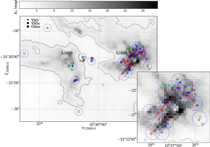
Figure 1. Spatial distribution of sources discussed in this work. Detected YSOs are shown as blue solid stars, YSO candidates as small magenta open circles, and other sources as green open squares. The YSOs not detected in our observations are shown as red open stars. The large blue circles indicate the position and size of representative VLBA fields used to observe our targets. The gray scale represents the extinction map obtained as part of the COMPLETE project (Ridge et al. 2006), based on 2MASS data (Skrutskie et al. 2006). The gray contour indicates an  of 4. The inset shows an enlargement of the Lynds 1688 area.
Download figure:
Standard image High-resolution imageThe observations were organized into various observing sessions, each with a different code, during which one or two pointing positions were observed (Table 1). The observing sessions consisted of cycles alternating between the target(s) and the main phase calibrator, J1627-2427: {target—J1627-2427} for single-target sessions, and {target 1—J1627-2427—target 2—J1627-2427} for those sessions where two targets were observed simultaneously. The target to calibrator angular separations were in the range of 0 1 for sources in Lynds 1688 to 12 for targets in the streamers. The on-source time was ∼110 s for each target and ∼50 s for the calibrator in every cycle. The total on-source time during each observing session was ∼1.6 hr in projects that observed at 8 GHz, and ∼1 hr at 5 GHz. Scans on the secondary calibrators, J1625-2417, J1625-2527, and J1633-2557, were also taken every ∼50 minutes during the observations. Unfortunately, one of the secondary calibrators, J1625-2417, was too weak to be detected in any of our observations at both 5 and 8 GHz. Finally, geodetic blocks were also included in each project, usually observed before and after the regular session.
The data reduction was done using AIPS (Greisen 2003) and following standard procedures for phase referencing VLBA observations. Initial calibration was performed as follows. Scans having elevations below 10° were flagged. The delays introduced by the ionospheric content were removed, and corrections to the Earth Orientation Parameters used by the correlator were then applied. Corrections for the rotation of the RCP and LCP feeds, as well as for voltage offsets in the samplers, were also applied. Amplitude calibration was done with the  method, using the provided gain curves and system temperatures to derive the System Equivalent Flux Density (SEFD) of each antenna. Instrumental single-band delays were then determined and removed using fringes detected on a single scan on the calibrator J1625-2527 or J1627-2427. Global fringe fitting was run on the main phase calibrator in order to find residual phase rates. This was done in two steps. First we used the task FRING without giving a specific source model, applied the solutions derived, and split and imaged the phase calibrator data. Then we ran FRING again on the data set with all the calibration applied except global fringe fitting, and using as a source model the self-calibrated image of the phase calibrator. Finally, the phase calibrator was phase-referenced to itself, and the secondary calibrators, as well as the program sources, were phase-referenced to the phase calibrator. The rms errors in source positions achieved with this initial calibration were as good as 0.01–0.02 mas for the strongest sources (a few mJy in flux density), and of the order of 0.1–0.3 mas for sub-mJy sources. However, these errors misrepresent the true errors because they do not incorporate systematic errors, which are dominated by unmodelled tropospheric zenith delays, ionospheric content delays, and atmospheric fluctuations above the VLBA antennas (Pradel et al. 2006).
Two calibration strategies can be adopted in order to deal with these systematic errors. One method consists in removing the tropospheric and clock errors using the all-sky calibrator blocks (Reid & Brunthaler 2004). These blocks consisted of observations of many calibrators over a wide range of elevations taken with 512 MHz total bandwidth covered by 16 IFs. The multi-band delay (i.e., the phase slope with frequency) was derived for each scan and antenna, and used to model the clock and zenith-path delay errors using the AIPS task DELZN. The corrections were then exported and applied to the phase referencing data set before global fringe fitting. The second method uses the scans on the secondary calibrators to determine the phase gradient across the sky. The data of the secondary calibrators are split and self-calibrated after initial and DELZN corrections are applied. The position offsets of the secondary calibrators from their respective phase centers are determined and removed, and residual phases are determined for all calibrators with the task CALIB. Finally, the AIPS task ATMCA is used to determine the phase gradients across the sky and then to correct the phase of all sources. We found that the corrections incorporated with DELZN decreased the rms error positions by a factor of up to ∼2 when applied to sources at more than 1° from the main calibrator. On the other hand, the non-detection of the secondary calibrator J1625-2417 prevented us from applying the corrections from ATMCA in most projects. We attempted to derive these corrections using the only detected calibrators J1627-2427 and J1625-2527, but this was limited to targets that are in line (within an angle of  ) with the two calibrators, and no significant improvement in the rms position error or image quality was achieved. Consequently, for the epochs taken during the fall of 2015 and spring of 2016, we replaced the secondary calibrator J1625-2417 with J1633-2557. This calibrator is well detected at both 5 and 8 GHz, and enabled us to apply the ATMCA corrections in the most recent projects. After application of ATMCA, the rms error of the position decreased, in some cases, to a quarter of its original value.
For observations where several phase centers are observed within a given primary beam, the calibration strategy described previously was applied to the primary phase center data. The other phase center data were calibrated by simply copying the final calibration (CL) tables, after appropriate editing with the AIPS task TABED to account for different source ID numbering.
Finally, we imaged the calibrated visibilities using a pixel size in the range of 50–100 μas and pure natural weighting (ROBUST = +5 in AIPS). We constructed maps as large as  to search for our sources. Typical angular resolutions are 4 mas × 2 mas (∼0.4 au at the distance of Ophiuchus) and 3 mas × 0.9 mas (∼0.3 au) at 5 and 8 GHz, respectively. The best noise level was achieved in the images at 5 GHz, and was of order of
  . The fluxes of sources observed in data with multiple field centers were corrected for primary beam attenuation. In doing this, we assumed that the primary beam response of the VLBA 25 m antennas is similar to that for the VLA 25 m antennas. The new AIPS task CLVLB, which incorporates antenna beam parameters for the VLBA, could be used for this purpose, but its performance is still being tested.
3. VLBA DETECTIONS
In Table 2 we list the YSOs detected in the Ophiuchus region. Columns (1) and (2) give the VLA position of the sources and their names, respectively. We report sources with flux densities above a 6σ detection threshold if they are detected in only one epoch. On the other hand, for sources with more than one detection, a threshold (in individual epochs) of  was used. We give the minimum and maximum total flux densities measured at both frequencies in columns (3) to (6), but we note that some sources were not observed at 8 GHz. In epochs where sources were observed but not detected, we give an upper flux density limit of 3σ. Six objects are resolved into multiple components; for those, we report the flux densities for each component separately. Brightness temperature (see Appendix
Table 2. Detected YSOs
| GBS-VLA | Other | Minimum Flux | Maximum Flux | Minimum Flux | Maximum Flux | log [Tb (K) ] | SED | Num. of | AV |
|---|---|---|---|---|---|---|---|---|---|
| Namea | Identifier | at 5 GHz (mJy) | at 5 GHz (mJy) | at 8 GHz (mJy) | at 8 GHz (mJy) | Class | Detc./Obs. | ||
| (1) | (2) | (3) | (4) | (5) | (6) | (7) | (8) | (9) | (10) |
| J162556.09-243015.3 | WLY2-11a | 0.13 ± 0.05 | 0.27 ± 0.06 | ⋯ | >7.0 | Class III | 4/5 | 13 | |
| J162556.09-243015.3 | WLY2-11b | 0.86 ± 0.05 | 0.60 ± 0.09 | 7.9 | ⋯ | 2/5 | ⋯ | ||
| J162557.51-243032.1 | YLW24 | 0.21 ± 0.05 | 1.35 ± 0.06 | 0.25 ± 0.06 | 8.0 | Class III | 4/5 | 13 | |
| J162603.01-242336.4 | DOAR21 | 1.98 ± 0.11 | 14.97 ± 0.14 | 4.13 ± 0.07 | 5.66 ± 0.07 | 9.2 | Class III | 7/7 | 12 |
| J162616.84-242223.5 | LFAMP1 | 0.15 ± 0.06 | 0.47 ± 0.04 | ⋯ | 6.8 | Class II | 2/6 | 20 | |
| J162622.38-242253.3 | LFAM2 | 0.30 ± 0.05 | 0.38 ± 0.07 | <0.09 | >6.7 | Class II | 3/7 | 20 | |
| J162625.62-242429.2 | LFAM4 | 0.66 ± 0.12 | <0.12 | >6.9 | Class I | 1/14 | 17 | ||
| J162629.67-241905.8 | LFAM8 | 0.37 ± 0.06 | 1.18 ± 0.13 | 0.26 ± 0.07 | 0.30 ± 0.05 | 7.3 | Class III | 7/9 | 19 |
| J162634.17-242328.4 | S1b | 5.56 ± 0.15 | 7.58 ± 0.07 | 3.27 ± 0.14 | 9.2 | Class III | 8/8 | 18 | |
| J162642.44-242626.1 | LFAM15a | 0.28 ± 0.05 | 0.93 ± 0.06 | 0.25 ± 0.06 | 1.50 ± 0.06 | 7.8 | Class III | 10/10 | 18 |
| J162642.44-242626.1 | LFAM15b | 0.15 ± 0.05 | 0.35 ± 0.07 | 0.18 ± 0.05 | 1.13 ± 0.05 | 6.8 | ⋯ | 7/10 | ⋯ |
| J162643.76-241633.4 | VSGG11a | 0.95 ± 0.04 | 1.53 ± 0.20 | ⋯ | 8.9 | Class III | 7/7 | 14 | |
| J162643.76-241633.4 | VSGG11b | 0.58 ± 0.06 | 0.82 ± 0.05 | ⋯ | 7.7 | ⋯ | 3/7 | ⋯ | |
| J162649.23-242003.3 | LFAM18 | 0.12 ± 0.03 | 1.23 ± 0.07 | <0.09 | 7.6 | Class III | 5/9 | 18 | |
| J162651.69-241441.5 | VSSG10 | 0.53 ± 0.07 | <0.06 | 7.1 | ⋯ | 1/5 | 12 | ||
| J162705.16-242007.8 | VSSG21 | 3.69 ± 0.07 | <0.09 | 8.4 | Class III | 1/11 | 19 | ||
| J162718.17-242852.9 | YLW12Ba | 0.70 ± 0.06 | 1.49 ± 0.05 | 0.84 ± 0.05 | 4.10 ± 0.08 | 8.7 | Class III | 9/9 | 26 |
| J162718.17-242852.9 | YLW12Bb | 0.42 ± 0.06 | 9.89 ± 0.11 | 1.19 ± 0.08 | 1.33 ± 0.05 | 8.9 | ⋯ | 9/9 | ⋯ |
| J162718.17-242852.9 | YLW12Bc | 0.45 ± 0.06 | 1.16 ± 0.09 | 0.17 ± 0.04 | 0.74 ± 0.08 | 7.8 | ⋯ | 7/9 | ⋯ |
| J162719.50-244140.3 | YLW13A | 0.35 ± 0.05 | 0.31 ± 0.08 | 0.71 ± 0.07 | 7.0 | Class III | 3/11 | 22 | |
| J162721.81-244335.9 | ROXN39a | 0.22 ± 0.07 | 1.44 ± 0.07 | 0.24 ± 0.06 | 0.44 ± 0.08 | 7.9 | Class III | 7/15 | 20 |
| J162721.81-244335.9 | ROXN39b | 0.22 ± 0.05 | 0.81 ± 0.06 | 0.57 ± 0.09 | 7.6 | ⋯ | 5/15 | ⋯ | |
| J162724.19-242929.8 | GY257 | 0.97 ± 0.06 | <0.09 | >7.0 | Class III | 1/8 | 13 | ||
| J162726.90-244050.8 | YLW15 | 0.18 ± 0.04 | 0.25 ± 0.08 | 0.23 ± 0.08 | 0.33 ± 0.06 | 7.1 | Class I | 5/11 | 25 |
| J162730.82-244727.2 | DROXO71 | 0.30 ± 0.05 | 0.91 ± 0.05 | 0.60 ± 0.07 | 1.15 ± 0.09 | 8.0 | Class III | 8/9 | 8 |
| J162804.65-243456.6 | ROXN78 | 0.38 ± 0.04 | <0.12 | >6.6 | Class II | 1/4 | 20 | ||
| J163035.63-243418.9 | SFAM87a | 0.48 ± 0.05 | 2.64 ± 0.09 | ⋯ | 8.1 | CTTS | 4/4 | 3 | |
| J163035.63-243418.9 | SFAM87b | 0.28 ± 0.06 | 1.35 ± 0.06 | ⋯ | 7.8 | ⋯ | 3/4 | ⋯ | |
| J163115.01-243243.9 | ROX42B | 0.21 ± 0.06 | 0.38 ± 0.08 | <0.12 | 7.0 | WTTS | 2/5 | 3 | |
| J163120.18-243001.0 | ROX43B | 0.20 ± 0.05 | 1.20 ± 0.08 | <0.12 | >7.1 | WTTS | 3/5 | 3 | |
| J163152.10-245615.7 | LDN1689IRS5 | 0.23 ± 0.05 | 3.17 ± 0.08 | 0.64 ± 0.07 | 8.3 | FS | 4/4 | 18 | |
| J163200.97-245643.3 | WLY2-67 | 0.18 ± 0.05 | 0.41 ± 0.07 | ⋯ | >6.6 | Class I | 3/3 | 14 | |
| J163211.79-244021.8 | DOAR51a | 0.40 ± 0.07 | 3.14 ± 0.06 | 0.69 ± 0.08 | 8.5 | WTTS/Class II | 7/7 | 8 | |
| J163211.79-244021.8 | DOAR51b | 0.24 ± 0.06 | 0.68 ± 0.07 | 0.47 ± 0.08 | 7.6 | ⋯ | 7/7 | ||
Notes. Reported sources have flux densities greater than  and
and  in the cases of one or several detections, respectively. Non-detections are indicated by giving an upper flux density limit of
  .
.
Download table as: ASCIITypeset image
4. ASTROMETRY
For all the objects detected with the VLBA, we have measured the source positions at each epoch by fitting two-dimensional Gaussians to the images, using the task JMFIT in AIPS. The resulting values are listed in Table 3. Having identified single, double, and multiple sources in our images, we used different approaches for the determination of the source astrometric parameters. We will first describe the approach followed for sources that appear to be single stars, or sources that show evidence of multiplicity but for which we do not have enough data to perform a more complex analysis.
Table 3. Measured Source Positions
| Julian Day | α (J2000.0) |

|
δ (J2000.0) |

|
|---|---|---|---|---|
| DROXO71 | ||||
| 2456011.96538 | 16 27 30.83414340 | 0.00000470 | −24 47 27.142107 | 0.000161 |
| 2456172.52613 | 16 27 30.83298666 | 0.00000234 | −24 47 27.153542 | 0.000071 |
| 2456471.70936 | 16 27 30.83302924 | 0.00000177 | −24 47 27.178102 | 0.000063 |
| 2456537.53271 | 16 27 30.83267868 | 0.00000191 | −24 47 27.182477 | 0.000065 |
| 2456718.03765 | 16 27 30.83359624 | 0.00000260 | −24 47 27.198462 | 0.000085 |
| 2456937.93345 | 16 27 30.83241321 | 0.00000472 | −24 47 27.212846 | 0.000216 |
| 2457081.04343 | 16 27 30.83323569 | 0.00000437 | −24 47 27.227091 | 0.000170 |
| 2457473.99603 | 16 27 30.83275199 | 0.00000469 | −24 47 27.256316 | 0.000188 |
| YLW13A | ||||
| 2456026.92477 | 16 27 19.49265640 | 0.00000349 | −24 41 40.735293 | 0.000105 |
| 2457097.02778 | 16 27 19.50365400 | 0.00001071 | −24 41 40.786841 | 0.000421 |
| 2457281.47003 | 16 27 19.49036366 | 0.00000974 | −24 41 40.828186 | 0.000183 |
| ROXN39 | ||||
| First source: | ||||
| 2456026.92477 | 16 27 21.81663353 | 0.00000626 | −24 43 35.989095 | 0.000146 |
| 2456748.92808 | 16 27 21.81566119 | 0.00000699 | −24 43 36.052317 | 0.000246 |
| 2457269.55653 | 16 27 21.81365382 | 0.00000174 | −24 43 36.095543 | 0.000068 |
| 2457281.47003 | 16 27 21.81365131 | 0.00000380 | −24 43 36.096674 | 0.000110 |
| 2457300.44295 | 16 27 21.81366628 | 0.00001385 | −24 43 36.098921 | 0.000329 |
| 2457467.95944 | 16 27 21.81426003 | 0.00000653 | −24 43 36.115527 | 0.000252 |
| 2457473.99603 | 16 27 21.81422633 | 0.00000534 | −24 43 36.115494 | 0.000195 |
| Second source: | ||||
| 2456748.92808 | 16 27 21.81377141 | 0.00000373 | −24 43 36.049837 | 0.000135 |
| 2456899.06892 | 16 27 21.81269783 | 0.00000865 | −24 43 36.052231 | 0.000272 |
| 2456937.93345 | 16 27 21.81279168 | 0.00001167 | −24 43 36.054796 | 0.000340 |
| 2457467.95944 | 16 27 21.81361924 | 0.00000366 | −24 43 36.075851 | 0.000106 |
| 2457473.99603 | 16 27 21.81361906 | 0.00000654 | −24 43 36.075317 | 0.000348 |
| YLW15 | ||||
| 2456026.92477 | 16 27 26.91975530 | 0.00000512 | −24 40 51.171077 | 0.000169 |
| 2456727.04112 | 16 27 26.91809446 | 0.00000928 | −24 40 51.223581 | 0.000233 |
| 2456748.92808 | 16 27 26.91792129 | 0.00001583 | −24 40 51.225402 | 0.000707 |
| 2457465.02060 | 16 27 26.91614817 | 0.00000759 | −24 40 51.276500 | 0.000342 |
| 2457467.95944 | 16 27 26.91612508 | 0.00000712 | −24 40 51.276834 | 0.000241 |
| GBS-VLA J162547.68-243735.7 | ||||
| 2456038.89200 | 16 25 47.68461899 | 0.00000324 | −24 37 35.718454 | 0.000151 |
| 2456221.39490 | 16 25 47.68461690 | 0.00000795 | −24 37 35.718318 | 0.000258 |
| 2456742.00017 | 16 25 47.68465538 | 0.00000741 | −24 37 35.718683 | 0.000312 |
| ROXN78 | ||||
| 2456730.03293 | 16 28 04.64323318 | 0.00000338 | −24 34 56.574659 | 0.000153 |
| YLW12B | ||||
| First source: | ||||
| 2453529.77467 | 16 27 18.17199790 | 0.00000343 | −24 28 52.790647 | 0.000136 |
| 2453887.79448 | 16 27 18.17278283 | 0.00000290 | −24 28 52.816450 | 0.000123 |
| 2456058.83738 | 16 27 18.17634770 | 0.00000188 | −24 28 52.966427 | 0.000074 |
| 2456269.26236 | 16 27 18.17718912 | 0.00000086 | −24 28 52.988798 | 0.000037 |
| 2456538.52830 | 16 27 18.17625293 | 0.00000233 | −24 28 53.000965 | 0.000096 |
| 2456720.03219 | 16 27 18.17804747 | 0.00000520 | −24 28 53.020088 | 0.000168 |
| 2456813.77622 | 16 27 18.17770160 | 0.00000143 | −24 28 53.029251 | 0.000049 |
| 2456943.42054 | 16 27 18.17733336 | 0.00000136 | −24 28 53.037170 | 0.000051 |
| 2457084.03523 | 16 27 18.17785280 | 0.00000290 | −24 28 53.041694 | 0.000105 |
| 2457302.43748 | 16 27 18.17777858 | 0.00000244 | −24 28 53.063201 | 0.000093 |
| 2457506.87788 | 16 27 18.17832802 | 0.00000112 | −24 28 53.079027 | 0.000040 |
| Second source: | ||||
| 2453529.77467 | 16 27 18.17173883 | 0.00000540 | −24 28 52.791325 | 0.000204 |
| 2453887.79448 | 16 27 18.17266976 | 0.00000411 | −24 28 52.810830 | 0.000122 |
| 2456058.83738 | 16 27 18.17665980 | 0.00000125 | −24 28 52.971988 | 0.000050 |
| 2456269.26236 | 16 27 18.17625269 | 0.00000295 | −24 28 52.979221 | 0.000124 |
| 2456538.52830 | 16 27 18.17657726 | 0.00000150 | −24 28 53.003249 | 0.000053 |
| 2456720.03219 | 16 27 18.17732771 | 0.00000412 | −24 28 53.015451 | 0.000142 |
| 2456813.77622 | 16 27 18.17673865 | 0.00000274 | −24 28 53.018125 | 0.000099 |
| 2456943.42054 | 16 27 18.17671228 | 0.00000435 | −24 28 53.026377 | 0.000135 |
| 2457084.03523 | 16 27 18.17822254 | 0.00000035 | −24 28 53.046405 | 0.000013 |
| 2457302.43748 | 16 27 18.17686941 | 0.00000315 | −24 28 53.053913 | 0.000128 |
| 2457506.87788 | 16 27 18.17801911 | 0.00000161 | −24 28 53.071326 | 0.000059 |
| Third source: | ||||
| 2453529.77467 | 16 27 18.16380766 | 0.00000229 | −24 28 52.878764 | 0.000071 |
| 2453818.98287 | 16 27 18.16367158 | 0.00000473 | −24 28 52.899861 | 0.000168 |
| 2456058.83738 | 16 27 18.15802440 | 0.00000540 | −24 28 53.043846 | 0.000282 |
| 2456269.26236 | 16 27 18.15742392 | 0.00000451 | −24 28 53.055984 | 0.000204 |
| 2456538.52830 | 16 27 18.15629959 | 0.00000497 | −24 28 53.072046 | 0.000126 |
| 2456813.77622 | 16 27 18.15608788 | 0.00000692 | −24 28 53.090076 | 0.000206 |
| 2457084.03523 | 16 27 18.15614139 | 0.00000292 | −24 28 53.109045 | 0.000096 |
| 2457302.43748 | 16 27 18.15467809 | 0.00000502 | −24 28 53.120030 | 0.000143 |
| 2457506.87788 | 16 27 18.15498736 | 0.00000543 | −24 28 53.134508 | 0.000170 |
| GY257 | ||||
| 2457506.87788 | 16 27 24.19599570 | 0.00000199 | −24 29 29.992344 | 0.000075 |
| LFAM15 | ||||
| First source: | ||||
| 2453617.53443 | 16 26 42.44072639 | 0.00000589 | −24 26 26.085858 | 0.000142 |
| 2453714.26955 | 16 26 42.44106573 | 0.00000587 | −24 26 26.090142 | 0.000259 |
| 2453796.04568 | 16 26 42.44134043 | 0.00000399 | −24 26 26.096076 | 0.000106 |
| 2456059.83431 | 16 26 42.43834146 | 0.00000119 | −24 26 26.270103 | 0.000040 |
| 2456270.25963 | 16 26 42.43790745 | 0.00000641 | −24 26 26.280485 | 0.000161 |
| 2456538.52830 | 16 26 42.43667908 | 0.00000321 | −24 26 26.294376 | 0.000107 |
| 2456720.03219 | 16 26 42.43733099 | 0.00000340 | −24 26 26.312356 | 0.000119 |
| 2456813.77622 | 16 26 42.43676227 | 0.00000259 | −24 26 26.323559 | 0.000087 |
| 2456943.42054 | 16 26 42.43645660 | 0.00000488 | −24 26 26.335835 | 0.000178 |
| 2457084.03523 | 16 26 42.43733727 | 0.00000560 | −24 26 26.348959 | 0.000259 |
| 2457302.43748 | 16 26 42.43619859 | 0.00000350 | −24 26 26.361949 | 0.000215 |
| 2457473.99603 | 16 26 42.43681431 | 0.00000819 | −24 26 26.372860 | 0.000381 |
| 2457506.87788 | 16 26 42.43657742 | 0.00000354 | −24 26 26.374173 | 0.000146 |
| Second source: | ||||
| 2456059.83431 | 16 26 42.43746443 | 0.00000139 | −24 26 26.259340 | 0.000047 |
| 2456270.25963 | 16 26 42.43721529 | 0.00000590 | −24 26 26.278386 | 0.000163 |
| 2456720.03219 | 16 26 42.43759083 | 0.00001060 | −24 26 26.317776 | 0.000382 |
| 2456813.77622 | 16 26 42.43677820 | 0.00000775 | −24 26 26.316132 | 0.000259 |
| 2456943.42054 | 16 26 42.43601697 | 0.00000783 | −24 26 26.320697 | 0.000297 |
| 2457302.43748 | 16 26 42.43531577 | 0.00001382 | −24 26 26.348716 | 0.000510 |
| 2457506.87788 | 16 26 42.43578894 | 0.00001213 | −24 26 26.368869 | 0.000282 |
| DOAR21 | ||||
| 2453621.52350 | 16 26 03.01891197 | 0.00000724 | −24 23 36.343197 | 0.000148 |
| 2453691.33229 | 16 26 03.01889886 | 0.00000304 | −24 23 36.349153 | 0.000063 |
| 2453744.18763 | 16 26 03.01910860 | 0.00000745 | −24 23 36.355709 | 0.000207 |
| 2453755.15740 | 16 26 03.01918629 | 0.00000284 | −24 23 36.355807 | 0.000115 |
| 2453822.97193 | 16 26 03.01896398 | 0.00000511 | −24 23 36.361907 | 0.000138 |
| 2453890.78627 | 16 26 03.01818785 | 0.00000166 | −24 23 36.364290 | 0.000075 |
| 2453971.56511 | 16 26 03.01698794 | 0.00000267 | −24 23 36.369931 | 0.000114 |
| 2454092.23452 | 16 26 03.01768929 | 0.00000161 | −24 23 36.380009 | 0.000052 |
| 2454321.60671 | 16 26 03.01610693 | 0.00000490 | −24 23 36.395975 | 0.000109 |
| 2454331.07942 | 16 26 03.01612164 | 0.00000175 | −24 23 36.395067 | 0.000052 |
| 2454353.51917 | 16 26 03.01600351 | 0.00000262 | −24 23 36.398021 | 0.000057 |
| 2454365.48657 | 16 26 03.01588946 | 0.00000202 | −24 23 36.398070 | 0.000067 |
| 2456158.56345 | 16 26 03.00879650 | 0.00000023 | −24 23 36.532098 | 0.000008 |
| 2456271.25813 | 16 26 03.00899222 | 0.00000045 | −24 23 36.541056 | 0.000014 |
| 2456537.53271 | 16 26 03.00730547 | 0.00000110 | −24 23 36.559579 | 0.000037 |
| 2456718.03765 | 16 26 03.00766323 | 0.00000030 | −24 23 36.575357 | 0.000010 |
| 2456937.93345 | 16 26 03.00579982 | 0.00000097 | −24 23 36.589569 | 0.000036 |
| 2457081.04343 | 16 26 03.00621579 | 0.00000166 | −24 23 36.602285 | 0.000058 |
| 2457300.44295 | 16 26 03.00441795 | 0.00000725 | −24 23 36.615740 | 0.000215 |
| LFAM8 | ||||
| 2456180.50470 | 16 26 29.67379969 | 0.00000658 | −24 19 05.899181 | 0.000225 |
| 2456283.22537 | 16 26 29.67437563 | 0.00000298 | −24 19 05.908297 | 0.000094 |
| 2456537.53271 | 16 26 29.67335645 | 0.00000458 | −24 19 05.927633 | 0.000138 |
| 2457081.04343 | 16 26 29.67375046 | 0.00000292 | −24 19 05.974041 | 0.000131 |
| 2457300.44295 | 16 26 29.67253899 | 0.00000614 | −24 19 05.990153 | 0.000254 |
| 2457449.06429 | 16 26 29.67333716 | 0.00000274 | −24 19 06.003299 | 0.000093 |
| 2457452.05609 | 16 26 29.67333731 | 0.00000416 | −24 19 06.004169 | 0.000133 |
| VSSG10 | ||||
| 2457449.06429 | 16 26 51.69086628 | 0.00000458 | −24 14 41.978736 | 0.000196 |
| YLW24 | ||||
| 2456258.29307 | 16 25 57.51212530 | 0.00000469 | −24 30 32.114725 | 0.000187 |
| 2456755.96194 | 16 25 57.51177560 | 0.00000627 | −24 30 32.152014 | 0.000205 |
| 2457141.90491 | 16 25 57.51110685 | 0.00000164 | −24 30 32.177539 | 0.000068 |
| 2457452.05609 | 16 25 57.51095598 | 0.00000448 | −24 30 32.199319 | 0.000150 |
| WLY2-11 | ||||
| First source: | ||||
| 2456755.96194 | 16 25 56.09115161 | 0.00000906 | −24 30 15.304290 | 0.000213 |
| 2457141.90491 | 16 25 56.09021133 | 0.00000936 | −24 30 15.334454 | 0.000522 |
| 2457265.56761 | 16 25 56.08917305 | 0.00001081 | −24 30 15.340167 | 0.000341 |
| 2457452.05609 | 16 25 56.08988393 | 0.00000486 | −24 30 15.353840 | 0.000178 |
| Second source: | ||||
| 2456258.29307 | 16 25 56.09091678 | 0.00000596 | −24 30 15.259179 | 0.000122 |
| 2457452.05609 | 16 25 56.09085688 | 0.00000182 | −24 30 15.339724 | 0.000071 |
| S1 | ||||
| First source: | ||||
| 2453545.73099 | 16 26 34.17395362 | 0.00000172 | −24 23 28.427300 | 0.000057 |
| 2453628.50402 | 16 26 34.17368732 | 0.00000218 | −24 23 28.432353 | 0.000096 |
| 2453722.24761 | 16 26 34.17436628 | 0.00000096 | −24 23 28.441953 | 0.000041 |
| 2453810.00745 | 16 26 34.17465184 | 0.00000263 | −24 23 28.451876 | 0.000080 |
| 2453889.78900 | 16 26 34.17402527 | 0.00000117 | −24 23 28.456156 | 0.000046 |
| 2453969.57055 | 16 26 34.17330377 | 0.00000147 | −24 23 28.462699 | 0.000057 |
| 2454256.78420 | 16 26 34.17389517 | 0.00000046 | −24 23 28.479576 | 0.000016 |
| 2454260.77321 | 16 26 34.17405536 | 0.00000056 | −24 23 28.476906 | 0.000019 |
| 2454264.76220 | 16 26 34.17381615 | 0.00000041 | −24 23 28.479414 | 0.000014 |
| 2454268.75117 | 16 26 34.17387600 | 0.00000102 | −24 23 28.479414 | 0.000027 |
| 2454272.74050 | 16 26 34.17376304 | 0.00000050 | −24 23 28.480753 | 0.000018 |
| 2454276.72950 | 16 26 34.17380110 | 0.00000045 | −24 23 28.482369 | 0.000013 |
| 2454280.71866 | 16 26 34.17371870 | 0.00000069 | −24 23 28.481435 | 0.000025 |
| 2454284.70775 | 16 26 34.17367060 | 0.00000047 | −24 23 28.480848 | 0.000015 |
| 2456278.23902 | 16 26 34.17330156 | 0.00000072 | −24 23 28.630001 | 0.000022 |
| 2456537.53271 | 16 26 34.17211016 | 0.00000072 | −24 23 28.648873 | 0.000024 |
| 2456718.03765 | 16 26 34.17335985 | 0.00000064 | −24 23 28.661727 | 0.000022 |
| 2456937.93345 | 16 26 34.17244477 | 0.00000091 | −24 23 28.677542 | 0.000031 |
| 2457081.04343 | 16 26 34.17321517 | 0.00000070 | −24 23 28.692245 | 0.000023 |
| 2457300.44295 | 16 26 34.17207637 | 0.00000093 | −24 23 28.702186 | 0.000032 |
| 2457473.99603 | 16 26 34.17308895 | 0.00000032 | −24 23 28.718119 | 0.000012 |
| 2457506.87788 | 16 26 34.17292128 | 0.00000050 | −24 23 28.720701 | 0.000016 |
| Second source: | ||||
| 2453889.78900 | 16 26 34.17355935 | 0.00000304 | −24 23 28.458375 | 0.000076 |
| 2454272.74050 | 16 26 34.17202332 | 0.00000178 | −24 23 28.499403 | 0.000067 |
| 2454276.72950 | 16 26 34.17205479 | 0.00000249 | −24 23 28.500747 | 0.000087 |
| 2454280.71866 | 16 26 34.17195583 | 0.00000592 | −24 23 28.499485 | 0.000245 |
| LFAM4 | ||||
| 2456538.52830 | 16 26 25.62311834 | 0.00000460 | −24 24 29.340081 | 0.000167 |
| LFAM2 | ||||
| 2457081.04343 | 16 26 22.39009598 | 0.00000517 | −24 22 53.396808 | 0.000267 |
| 2457300.44295 | 16 26 22.38891477 | 0.00000858 | −24 22 53.410054 | 0.000331 |
| 2457473.99603 | 16 26 22.38959724 | 0.00000460 | −24 22 53.425842 | 0.000181 |
| VSSG21 | ||||
| 2456755.96194 | 16 27 05.16439110 | 0.00000056 | −24 20 08.102812 | 0.000024 |
| GBS-VLA J163151.93-245617.4 | ||||
| 2456409.87863 | 16 31 51.92835399 | 0.00000519 | −24 56 17.490313 | 0.000168 |
| 2456741.00290 | 16 31 51.92788684 | 0.00001420 | −24 56 17.512182 | 0.000360 |
| 2457449.06429 | 16 31 51.92686645 | 0.00000519 | −24 56 17.565067 | 0.000192 |
| GBS-VLA J163202.39-245710.0 | ||||
| 2456409.87863 | 16 32 02.39822000 | 0.00000432 | −24 57 10.343815 | 0.000154 |
| 2456741.00290 | 16 32 02.39823221 | 0.00002166 | −24 57 10.344630 | 0.000553 |
| LDN1689IRS5 | ||||
| 2456409.87863 | 16 31 52.11386300 | 0.00000351 | −24 56 16.009652 | 0.000093 |
| 2456741.00290 | 16 31 52.11363279 | 0.00000864 | −24 56 16.030780 | 0.000269 |
| 2457285.48390 | 16 31 52.11201000 | 0.00000095 | −24 56 16.062292 | 0.000034 |
| 2457449.06429 | 16 31 52.11274267 | 0.00000786 | −24 56 16.074290 | 0.000235 |
| GBS-VLA J163138.57-253220.0 | ||||
| 2456433.81310 | 16 31 38.57911827 | 0.00000420 | −25 32 20.078468 | 0.000158 |
| 2456541.52018 | 16 31 38.57910247 | 0.00001600 | −25 32 20.080138 | 0.000563 |
| 2456723.02399 | 16 31 38.57913786 | 0.00000345 | −25 32 20.076607 | 0.000137 |
| 2457309.41870 | 16 31 38.57913003 | 0.00000375 | −25 32 20.077101 | 0.000121 |
| ROX42B | ||||
| 2456560.49689 | 16 31 15.01221991 | 0.00001035 | −24 32 44.039658 | 0.000379 |
| 2457477.98511 | 16 31 15.01218127 | 0.00001539 | −24 32 44.101781 | 0.000549 |
| ROX43B | ||||
| 2456560.49689 | 16 31 20.18111995 | 0.00000200 | −24 30 01.018464 | 0.000076 |
| 2456731.03020 | 16 31 20.18256906 | 0.00000752 | −24 30 01.028170 | 0.000365 |
| 2457477.98511 | 16 31 20.18076137 | 0.00001494 | −24 30 01.082333 | 0.000455 |
| DOAR51 | ||||
| First source: | ||||
| 2456449.77302 | 16 32 11.79261358 | 0.00000197 | −24 40 21.924420 | 0.000089 |
| 2456539.52565 | 16 32 11.79223385 | 0.00000579 | −24 40 21.928946 | 0.000216 |
| 2456721.02946 | 16 32 11.79332766 | 0.00000435 | −24 40 21.943832 | 0.000148 |
| 2456946.41259 | 16 32 11.79248077 | 0.00000489 | −24 40 21.958212 | 0.000215 |
| 2457102.07550 | 16 32 11.79325983 | 0.00000059 | −24 40 21.971486 | 0.000023 |
| 2457309.41870 | 16 32 11.79227112 | 0.00000290 | −24 40 21.984119 | 0.000103 |
| 2457448.12863 | 16 32 11.79303712 | 0.00000227 | −24 40 21.997374 | 0.000079 |
| Second source: | ||||
| 2456449.77302 | 16 32 11.79007110 | 0.00000269 | −24 40 21.944770 | 0.000109 |
| 2456539.52565 | 16 32 11.78935516 | 0.00001089 | −24 40 21.948446 | 0.000263 |
| 2456721.02946 | 16 32 11.78995501 | 0.00001231 | −24 40 21.961295 | 0.000497 |
| 2456946.41259 | 16 32 11.78863803 | 0.00000746 | −24 40 21.973309 | 0.000310 |
| 2457102.07550 | 16 32 11.78921243 | 0.00000357 | −24 40 21.982029 | 0.000146 |
| 2457309.41870 | 16 32 11.78806957 | 0.00000361 | −24 40 21.990150 | 0.000124 |
| 2457448.12863 | 16 32 11.78882778 | 0.00000293 | −24 40 21.999831 | 0.000118 |
| SFAM200 | ||||
| 2456458.74485 | 16 32 45.23630782 | 0.00000791 | −24 36 47.331480 | 0.000179 |
| 2456541.52018 | 16 32 45.23628708 | 0.00001362 | −24 36 47.332569 | 0.000400 |
| 2456723.02399 | 16 32 45.23630881 | 0.00000937 | −24 36 47.331435 | 0.000298 |
| SSTc2d J163027.7-243300 | ||||
| 2456731.03020 | 16 30 27.69715982 | 0.00000740 | −24 33 00.166706 | 0.000227 |
| 2457270.55380 | 16 30 27.69716395 | 0.00000719 | −24 33 00.166547 | 0.000347 |
| SFAM212 | ||||
| 2456174.52068 | 16 36 17.50047169 | 0.00000084 | −24 25 55.410771 | 0.000027 |
| 2456539.52565 | 16 36 17.50048182 | 0.00000235 | −24 25 55.411813 | 0.000080 |
| 2456721.02946 | 16 36 17.50043917 | 0.00000329 | −24 25 55.411946 | 0.000108 |
| 2456946.41259 | 16 36 17.50048274 | 0.00000525 | −24 25 55.412111 | 0.000178 |
| 2457102.07550 | 16 36 17.50047251 | 0.00000116 | −24 25 55.411264 | 0.000047 |
| LFAMP1 | ||||
| 2456718.03765 | 16 26 16.84931422 | 0.00000236 | −24 22 23.537591 | 0.000088 |
| 2456937.93345 | 16 26 16.84846826 | 0.00001253 | −24 22 23.550740 | 0.000517 |
| LFAM13 | ||||
| 2456720.03219 | 16 26 35.33007904 | 0.00001742 | −24 24 05.378855 | 0.000554 |
| 2456937.93345 | 16 26 35.33016006 | 0.00001436 | −24 24 05.378401 | 0.000281 |
| 2456943.42054 | 16 26 35.33013612 | 0.00000787 | −24 24 05.376639 | 0.000298 |
| 2457302.43748 | 16 26 35.33013402 | 0.00001301 | −24 24 05.377817 | 0.000371 |
| GBS-VLA J162718.25-243334.8 | ||||
| 2457084.03523 | 16 27 18.23431162 | 0.00000882 | −24 33 34.951660 | 0.000347 |
| SFAM130 | ||||
| 2456721.02946 | 16 32 10.77123123 | 0.00000769 | −24 38 27.498627 | 0.000233 |
| 2456946.41259 | 16 32 10.77132165 | 0.00001042 | −24 38 27.496690 | 0.000383 |
| 2457102.07550 | 16 32 10.77128863 | 0.00001343 | −24 38 27.497429 | 0.000317 |
| 2457309.41870 | 16 32 10.77126826 | 0.00000644 | −24 38 27.497571 | 0.000250 |
| SSTc2d J163211.1-243651 | ||||
| 2456539.52565 | 16 32 11.08492873 | 0.00000804 | −24 36 50.916471 | 0.000549 |
| 2456721.02946 | 16 32 11.08495049 | 0.00000963 | −24 36 50.915528 | 0.000274 |
| 2456946.41259 | 16 32 11.08491744 | 0.00000818 | −24 36 50.917097 | 0.000224 |
| 2457102.07550 | 16 32 11.08494017 | 0.00000383 | −24 36 50.915872 | 0.000177 |
| 2457309.41870 | 16 32 11.08495182 | 0.00000556 | −24 36 50.915556 | 0.000282 |
| GBS-VLA J163212.25-243643.7 | ||||
| 2457102.07550 | 16 32 12.24716110 | 0.00000524 | −24 36 43.555532 | 0.000196 |
| 2457309.41870 | 16 32 12.24719840 | 0.00001393 | −24 36 43.555066 | 0.000612 |
| GBS-VLA J163213.92-244407.8 | ||||
| 2457309.41870 | 16 32 13.92922573 | 0.00000974 | −24 44 07.782062 | 0.000186 |
| SSTc2d J163227.4-243951 | ||||
| 2456721.02946 | 16 32 27.40769338 | 0.00002030 | −24 39 51.454135 | 0.000725 |
| 2457102.07550 | 16 32 27.40765118 | 0.00000920 | −24 39 51.456859 | 0.000382 |
| 2457309.41870 | 16 32 27.40762110 | 0.00001175 | −24 39 51.455911 | 0.000659 |
| SSTc2d J163231.2-244014 | ||||
| 2457102.07550 | 16 32 31.16848721 | 0.00000770 | −24 40 14.638470 | 0.000295 |
| 2457309.41870 | 16 32 31.16851261 | 0.00000859 | −24 40 14.639088 | 0.000376 |
| GBS-VLA J162713.06-241817.0 | ||||
| 2457269.55653 | 16 27 13.06069106 | 0.00000787 | −24 18 17.090808 | 0.000338 |
| 2457465.02060 | 16 27 13.06072912 | 0.00001137 | −24 18 17.092477 | 0.000381 |
| ROC25 | ||||
| 2456555.51075 | 16 27 29.23368916 | 0.00000582 | −24 17 55.411620 | 0.000156 |
| 2456727.04112 | 16 27 29.23368444 | 0.00000273 | −24 17 55.411606 | 0.000073 |
| 2456899.06892 | 16 27 29.23371052 | 0.00000246 | −24 17 55.411246 | 0.000075 |
| 2457097.02778 | 16 27 29.23368684 | 0.00000476 | −24 17 55.411581 | 0.000139 |
| 2457269.55653 | 16 27 29.23368353 | 0.00000548 | −24 17 55.411757 | 0.000137 |
| ROC26 | ||||
| 2456555.51075 | 16 27 34.55992198 | 0.00000920 | −24 20 20.725049 | 0.000281 |
| 2456727.04112 | 16 27 34.55990816 | 0.00000510 | −24 20 20.724976 | 0.000176 |
| 2456899.06892 | 16 27 34.55991988 | 0.00000299 | −24 20 20.725208 | 0.000104 |
| 2457097.02778 | 16 27 34.55991770 | 0.00000610 | −24 20 20.725197 | 0.000177 |
| 2457269.55653 | 16 27 34.55988071 | 0.00000902 | −24 20 20.725929 | 0.000350 |
| SSTc2d J163032.3-243128 | ||||
| 2456560.49689 | 16 30 32.26027376 | 0.00000447 | −24 31 28.011713 | 0.000186 |
| 2456731.03020 | 16 30 32.26025039 | 0.00000216 | −24 31 28.012042 | 0.000067 |
| 2457270.55380 | 16 30 32.26027063 | 0.00000352 | −24 31 28.012434 | 0.000131 |
| ROC49 | ||||
| 2456560.49689 | 16 31 09.78490899 | 0.00000944 | −24 30 08.324997 | 0.000282 |
| 2456731.03020 | 16 31 09.78489672 | 0.00000537 | −24 30 08.325067 | 0.000171 |
| 2457270.55380 | 16 31 09.78491218 | 0.00000441 | −24 30 08.324410 | 0.000184 |
| SSTc2d J163033.2-243039 | ||||
| 2456731.03020 | 16 30 33.25165317 | 0.00000638 | −24 30 38.884059 | 0.000206 |
| GBS-VLA J163115.25-243313.8 | ||||
| 2456731.03020 | 16 31 15.25452244 | 0.00000545 | −24 33 13.781612 | 0.000281 |
| 2457477.98511 | 16 31 15.25455673 | 0.00002498 | −24 33 13.781713 | 0.000755 |
| ROC52 | ||||
| 2456560.49689 | 16 31 20.13897283 | 0.00000266 | −24 29 28.542211 | 0.000089 |
| 2456731.03020 | 16 31 20.13896190 | 0.00000060 | −24 29 28.542334 | 0.000023 |
| 2457270.55380 | 16 31 20.13897246 | 0.00000075 | −24 29 28.541947 | 0.000026 |
| SFAM87 | ||||
| First source: | ||||
| 2454620.78761 | 16 30 35.63476219 | 0.00000484 | −24 34 18.958646 | 0.000167 |
| 2454785.33715 | 16 30 35.63494522 | 0.00000500 | −24 34 18.970301 | 0.000172 |
| 2454877.08587 | 16 30 35.63580491 | 0.00000407 | −24 34 18.978334 | 0.000165 |
| 2456560.49689 | 16 30 35.63166911 | 0.00000102 | −24 34 19.064773 | 0.000040 |
| 2456731.03020 | 16 30 35.63203197 | 0.00000362 | −24 34 19.082480 | 0.000121 |
| 2457270.55380 | 16 30 35.62974397 | 0.00000151 | −24 34 19.139299 | 0.000050 |
| 2457477.98511 | 16 30 35.63098169 | 0.00000835 | −24 34 19.163958 | 0.000267 |
| Second source: | ||||
| 2454540.00885 | 16 30 35.63655437 | 0.00000135 | −24 34 18.935779 | 0.000053 |
| 2454620.78761 | 16 30 35.63568452 | 0.00000435 | −24 34 18.937621 | 0.000148 |
| 2454698.57472 | 16 30 35.63478278 | 0.00000464 | −24 34 18.939787 | 0.000147 |
| 2454785.33715 | 16 30 35.63468005 | 0.00000557 | −24 34 18.946096 | 0.000212 |
| 2454877.08587 | 16 30 35.63485533 | 0.00000211 | −24 34 18.954888 | 0.000079 |
| 2454967.83741 | 16 30 35.63402510 | 0.00000481 | −24 34 18.962548 | 0.000165 |
| 2456731.03020 | 16 30 35.63287869 | 0.00000291 | −24 34 19.118843 | 0.000116 |
| 2457270.55380 | 16 30 35.63143895 | 0.00000147 | −24 34 19.133256 | 0.000054 |
| 2457477.98511 | 16 30 35.63152547 | 0.00001503 | −24 34 19.142294 | 0.000522 |
| SSTc2d J163130.6-243352 | ||||
| 2456560.49689 | 16 31 30.62178183 | 0.00001008 | −24 33 51.512104 | 0.000239 |
| 2456731.03020 | 16 31 30.62181139 | 0.00000426 | −24 33 51.512137 | 0.000167 |
| 2457270.55380 | 16 31 30.62177163 | 0.00000812 | −24 33 51.511820 | 0.000319 |
| GBS-VLA J163036.26-243135.3 | ||||
| 2456560.49689 | 16 30 36.26501151 | 0.00000629 | −24 31 35.400645 | 0.000275 |
| 2456731.03020 | 16 30 36.26500965 | 0.00000206 | −24 31 35.401147 | 0.000078 |
| 2457270.55380 | 16 30 36.26502326 | 0.00000408 | −24 31 35.401258 | 0.000142 |
| VSGG11 | ||||
| First source: | ||||
| 2456722.00179 | 16 26 43.75569790 | 0.00000130 | −24 16 33.615170 | 0.000060 |
| 2456755.96194 | 16 26 43.75550380 | 0.00000342 | −24 16 33.618593 | 0.000139 |
| 2457141.90491 | 16 26 43.75454490 | 0.00000505 | −24 16 33.658504 | 0.000212 |
| 2457265.56761 | 16 26 43.75352207 | 0.00000313 | −24 16 33.670179 | 0.000132 |
| 2457285.48390 | 16 26 43.75347972 | 0.00000172 | −24 16 33.671690 | 0.000055 |
| 2457449.06429 | 16 26 43.75415819 | 0.00000107 | −24 16 33.691930 | 0.000043 |
| 2457452.05609 | 16 26 43.75415976 | 0.00000210 | −24 16 33.692895 | 0.000076 |
| Second source: | ||||
| 2457285.48390 | 16 26 43.75384015 | 0.00000355 | −24 16 33.678776 | 0.000123 |
| 2457449.06429 | 16 26 43.75459284 | 0.00000210 | −24 16 33.689691 | 0.000089 |
| 2457452.05609 | 16 26 43.75456000 | 0.00000788 | −24 16 33.689666 | 0.000349 |
| SSTc2d J163154.5-245217 | ||||
| 2456741.00290 | 16 31 54.49445738 | 0.00001834 | −24 52 17.136283 | 0.000774 |
| 2457449.06429 | 16 31 54.49438170 | 0.00001014 | −24 52 17.138334 | 0.000276 |
| WLY2-67 | ||||
| 2456741.00290 | 16 32 00.97871474 | 0.00001192 | −24 56 43.413340 | 0.000456 |
| 2457285.48390 | 16 32 00.97716307 | 0.00000733 | −24 56 43.446632 | 0.000312 |
| 2457449.06429 | 16 32 00.97790521 | 0.00001256 | −24 56 43.460244 | 0.000403 |
| LFAM18 | ||||
| 2456722.00179 | 16 26 49.22836555 | 0.00000789 | −24 20 03.414117 | 0.000375 |
| 2456755.96194 | 16 26 49.22819914 | 0.00000199 | −24 20 03.416423 | 0.000071 |
| 2457141.90491 | 16 26 49.22715919 | 0.00000817 | −24 20 03.438613 | 0.000336 |
| 2457265.56761 | 16 26 49.22608389 | 0.00000392 | −24 20 03.441434 | 0.000147 |
| 2457452.05609 | 16 26 49.22669248 | 0.00000861 | −24 20 03.449981 | 0.000452 |
| LFAM17 | ||||
| 2456722.00179 | 16 26 46.36011062 | 0.00001632 | −24 20 02.188965 | 0.000342 |
| 2456755.96194 | 16 26 46.36010779 | 0.00001240 | −24 20 02.191625 | 0.000382 |
| 2457141.90491 | 16 26 46.36005985 | 0.00001738 | −24 20 02.191462 | 0.000423 |
| 2457265.56761 | 16 26 46.35994120 | 0.00001558 | −24 20 02.192545 | 0.000467 |
| 2457452.05609 | 16 26 46.36005050 | 0.00001543 | −24 20 02.192970 | 0.000480 |
| GDS J162702.1-241928 | ||||
| 2456755.96194 | 16 27 02.15242055 | 0.00001218 | −24 19 27.915618 | 0.000350 |
| 2457141.90491 | 16 27 02.15241390 | 0.00000876 | −24 19 27.915343 | 0.000447 |
| 2457265.56761 | 16 27 02.15242622 | 0.00001325 | −24 19 27.915196 | 0.000502 |
| 2457452.05609 | 16 27 02.15240463 | 0.00000675 | −24 19 27.915947 | 0.000298 |
| SFAM127 | ||||
| 2456741.00290 | 16 31 59.36475311 | 0.00000244 | −24 56 39.800373 | 0.000088 |
| 2457285.48390 | 16 31 59.36476531 | 0.00000360 | −24 56 39.800194 | 0.000124 |
| SSTc2d J162540.9-244147 | ||||
| 2456742.00017 | 16 25 40.94715532 | 0.00001533 | −24 41 47.337014 | 0.000538 |
| SFAM12 | ||||
| 2456722.00179 | 16 26 33.48487742 | 0.00001057 | −24 12 16.100168 | 0.000479 |
| 2457285.48390 | 16 26 33.48605313 | 0.00001170 | −24 12 16.124239 | 0.000455 |
4.1. Single Stars
Source positions were modeled to derive the trigonometric parallax (ϖ), proper motion ( ,
,  ), and mean position (
 ,
,  ). The fits were performed by minimizing the associated
  (e.g., Loinard et al. 2007) and solving for the five astrometric elements simultaneously. For the errors in the positions at each epoch, we used the statistical errors provided by JMFIT, which roughly represent the expected theoretical precision of VLBA astrometry. However, systematic errors may significantly contribute to the astrometric accuracy (Pradel et al. 2006) and affect the derived astrometric parameters.
We estimate the systematic errors in two different ways: First, we use the empirical relation found by Pradel et al. (2006), according to which the VLBA astrometric accuracy scales linearly with the angular separation between the source and the phase calibrator. In the core, sources are separated from the phase calibrator, J1627-2427, by up to 04. Given this angular separation, and a typical declination of  , the expected VLBA rms astrometric errors
  are
are  as. For this calculation, we have assumed that the rms errors for source coordinates, VLBA station coordinates, Earth orientation parameters (EOPs), and wet tropospheric zenith-path delays all contribute together (Tables 3 and 4, and Equation (2) in Pradel et al. 2006).
The systematic errors were also estimated by quadratically adding an error to the statistical errors given by JMFIT until a reduced  of 1 was achieved in the astrometric fits. These systematic errors are in general several times larger than those predicted by the empirical relation. We note, however, that in their simulations, Pradel et al. (2006) assumed a full track on the source, while in our observations the source is tracked over less than 4 hr, resulting in a poorer
  coverage. We used the latter approach (based on a measured reduced
  ) to deal with systematic errors. As stated previously, these errors were added quadratically to the statistical errors of each individual epoch and used in the last iteration of the fits.
In the following subsections, we will comment separately on a few of the critical sources describing the additional data that were taken from the VLBA archive, when available, and detailing the quality of the fits. In Table 4, we provide the resulting astrometric parameters and distances for the complete sample. The corresponding measured source positions and best fits are shown in Figure 2.
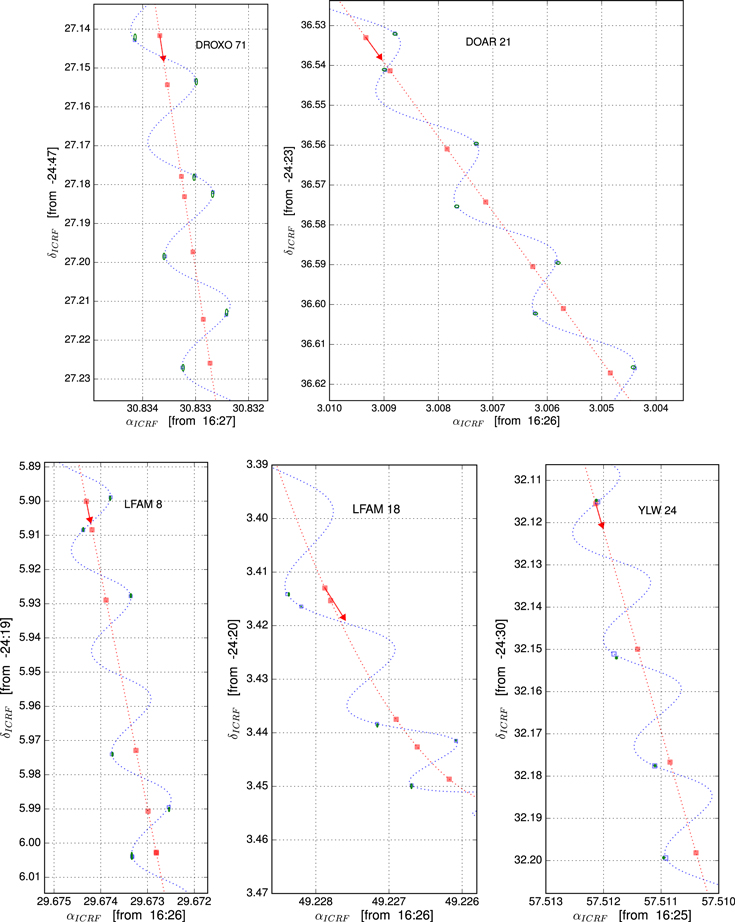
Download figure:
Standard image High-resolution image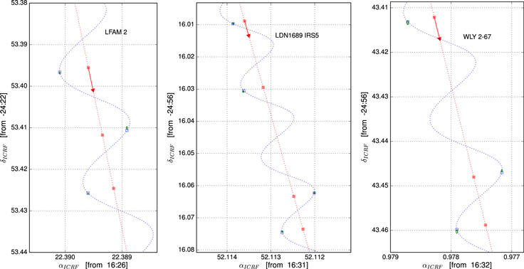
Figure 2. Observed positions and best fit for single sources. Measured positions are shown as green ellipses, the size of which represents the magnitude of the errors. The expected positions from the fit are shown as blue open squares. The blue dotted line is the full model, and the red line is the model with the parallax signature removed. The red squares indicate the position of the source expected from the model without parallax. When the systematic errors on source positions can be estimated from the fits, these are included in the error bars shown in the plots. The arrow shows the direction of position change over time.
Download figure:
Standard image High-resolution imageTable 4. Parallaxes and Proper Motions
| GBS-VLA | Other Identifier | Parallax |

|

|

|

|
Distance |
|---|---|---|---|---|---|---|---|
| Name | (mas) | (mas yr−1) | (mas yr−1) | (mas yr−2) | (mas yr−2) | (pc) | |
| (1) | (2) | (3) | (4) | (5) | (6) | (7) | (8) |
| J162556.09-243015.3 | WLY2-11 | 7.330 ± 0.112 | −9.78 ± 0.09 | −25.11 ± 0.20 | 0.94 ± 0.38 | 6.02 ± 0.83 | 136.4 ± 2.1 |
| J162557.51-243032.1 | YLW24 | 7.404 ± 0.143 | −7.26 ± 0.04 | −25.29 ± 0.07 | ⋯ | ⋯ | 135.1 ± 2.6 |
| J162603.01-242336.4 | DoAr21 | 7.385 ± 0.234 | −19.63 ± 0.19 | −26.92 ± 0.13 | ⋯ | ⋯ | 135.4 ± 4.3 |
| J162622.38-242253.3 | LFAM2 | 7.060 ± 0.072 | −5.64 ± 0.09 | −27.02 ± 0.30 | ⋯ | ⋯ | 141.6 ± 1.5 |
| J162629.67-241905.8 | LFAM8 | 7.246 ± 0.088 | −5.89 ± 0.06 | −29.54 ± 0.16 | ⋯ | ⋯ | 138.0 ± 1.7 |
| J162634.17-242328.4 | S1 | 7.249 ± 0.091 | −2.05 ± 0.02 | −26.72 ± 0.04 | ⋯ | ⋯ | 138.0 ± 1.7 |
| J162642.44-242626.1 | LFAM15 | 7.253 ± 0.054 | −6.31 ± 0.02 | −26.95 ± 0.05 | ⋯ | ⋯ | 137.9 ± 1.0 |
| J162643.76-241633.4 | VSSG11 | 7.160 ± 0.152 | −10.48 ± 0.16 | −38.99 ± 0.35 | 0.31 ± 0.65 | −1.54 ± 1.09 | 139.7 ± 3.0 |
| J162649.23-242003.3 | LFAM18 | 7.232 ± 0.068 | −11.62 ± 0.06 | −18.30 ± 0.15 | −0.10 ± 0.32 | 8.17 ± 0.84 | 138.3 ± 1.3 |
| J162718.17-242852.9 | YLW 12Bab | 7.230 ± 0.057 | 6.56 ± 0.02 | −26.26 ± 0.04 | −0.62 ± 0.01 | −0.17 ± 0.02 | 138.3 ± 1.1 |
| J162718.17-242852.9 | YLW 12Bca | 7.230 ± 0.057 | −11.23 ± 0.07 | −23.10 ± 0.10 | 0.19 ± 0.03 | 0.11 ± 0.05 | 138.3 ± 1.1 |
| J162721.81-244335.9 | ROXN39 | 7.317 ± 0.021 | −7.32 ± 0.31 | −26.21 ± 0.73 | ⋯ | ⋯ | 136.7 ± 0.4 |
| J162730.82-244727.2 | DROXO71 | 7.327 ± 0.125 | −4.41 ± 0.11 | −28.79 ± 0.33 | ⋯ | ⋯ | 136.5 ± 2.3 |
| J163035.63-243418.9 | SFAM 87 | 7.206 ± 0.080 | −7.69 ± 0.02 | −26.04 ± 0.04 | ⋯ | ⋯ | 138.8 ± 1.5 |
| J163152.10-245615.7 | LDN1689IRS5 | 6.676 ± 0.046 | −6.38 ± 0.03 | −22.74 ± 0.04 | ⋯ | ⋯ | 149.8 ± 1.0 |
| J163200.97-245643.3 | WLY2-67 | 6.616 ± 0.088 | −5.94 ± 0.12 | −24.08 ± 0.30 | ⋯ | ⋯ | 151.2 ± 2.0 |
| J163211.79-244021.8 | DoAr51 | 6.983 ± 0.050 | −4.80 ± 0.08 | −23.11 ± 0.11 | ⋯ | ⋯ | 143.2 ± 1.0 |
Note.
aParallax is fixed at the value obtained for YLW 12Bab when solving for the other astrometric parameters.Download table as: ASCIITypeset image
4.1.1. DROXO 71
The model that assumes a uniform and linear proper motion produces a good fit to the data. However, we discarded the last detection because it degrades the quality of the fit. We ignored the source of the error that may be introduced in this particular epoch, but we found that the "expected" position from the fit to the first seven epochs was on a sidelobe.
4.1.2. DoAr 21
DoAr 21 has been observed and detected at seven epochs. In addition to these observations, the source was observed with the VLBA prior to 2012 in projects BL128 (nine epochs from September 2005 to December 2006) and BT093 (eight epochs from 2007 July to 2007 September). Seven epochs from project BL128 were analyzed and published in Loinard et al. (2008). Because the observing and calibration strategy adopted for GOBELINS is not exactly the same as in Loinard et al. (2008), we performed a consistency check as follows. We downloaded, calibrated and revised these prior observations by applying the same calibration procedures as to the data from our own project. We note, however, that a large fraction of the observations taken between 2006 December and 2007 September involved very poor weather conditions (Table 5). Such conditions affected the image quality, and the rms error position was relatively high in comparison with that measured in observations collected under optimal weather. In the present analysis, we do not include the epochs when data were highly affected, and only five additional epochs to the seven reported by Loinard et al. (2008) were included. Hence a total of 12 epochs from 2005 September to 2007 September are considered in our analysis.
Table 5. Archive VLBA Data
| Project Code | Date of Observation | Source | Relevant Entries from the Observing Log |
|---|---|---|---|
| BL128 FA | 2005 Jun 07 | LFAM 15 | ⋯ |
| BL128 FB | 2005 Sep 03 | LFAM 15 | ⋯ |
| BL128 FC | 2005 Dec 09 | LFAM 15 | ⋯ |
| BL128 FD | 2006 Mar 01 | LFAM 15 | ⋯ |
| BL128 FGa | 2006 Dec 20 | DOAR 21 | PT may have some residual snow in the dish. |
| Cloudy at NL, LA, and PT. | |||
| LA weather: overcast and snowing. 2 inches of snow. | |||
| NL precipitation. | |||
| BL128 FF | 2006 Dec 22 | DOAR 21 | ⋯ |
| BT093 CAa | 2007 Jul 10 | DOAR 21 | Rain at NL, overcast SC, HN. |
| BT093 CBa | 2007 Jul 20 | DOAR 21 | SC out due to bad HVAC in vertex rm. LA raining. |
| KP 35+ mph wind caution. | |||
| BT093 CCa | 2007 Jul 31 | DOAR 21 | HN and BR unavailable for observing due to |
| scheduled maintenance visits. Raining at SC and FD. | |||
| BT093 CD | 2007 Aug 09 | DOAR 21 | ⋯ |
| BT093 CE | 2007 Aug 18 | DOAR 21 | ⋯ |
| BT093 CFa,b | 2007 Aug 29 | DOAR 21 | SC, NL cloudy. NL, OV windy. |
| BT093 CG | 2007 Sep 09 | DOAR 21 | ⋯ |
| BT093 CH | 2007 Sep 21 | DOAR 21 | ⋯ |
| BL128 DA | 2005 Jun 08 | YLW 12B | ⋯ |
| BL128 DG | 2005 Sep 11 | YLW 12B | ⋯ |
| BL128 DC | 2005 Dec 05 | YLW 12B | BR: not fringing, data not usable. |
| NL: slow to get on source. | |||
| BL128 DD | 2006 Mar 24 | YLW 12B | ⋯ |
| BL128 DE | 2006 Jun 01 | YLW 12B | ⋯ |
| BL128 DFa | 2006 Aug 27 | YLW 12B | Raining at FD, MK and HN. |
| BL128 GA | 2005 Jun 24 | S1 | ⋯ |
| BL128 GB | 2005 Sep 15 | S1 | ⋯ |
| BL128 GC | 2005 Dec 17 | S1 | ⋯ |
| BL128 GD | 2006 Mar 15 | S1 | ⋯ |
| BL128 GE | 2006 Jun 03 | S1 | Raining at HN. |
| KP subreflector not moving to any position in ROTATION. | |||
| KP antenna is removed from observing. | |||
| HN disabled ROTATION axis, subreflector is | |||
| About 6 counts off in ROTATION position. | |||
| BL128 GF | 2006 Aug 22 | S1 | ⋯ |
| BT093 BA | 2007 Jun 05 | S1 | ⋯ |
| BT093 BB | 2007 Jun 09 | S1 | FD is on generator power, not in observation. |
| PT HC2 FIFO error. | |||
| BT093 BC | 2007 Jun 13 | S1 | ⋯ |
| BT093 BD | 2007 Jun 17 | S1 | SC, HN, NL overcast. |
| SC precipitation. | |||
| BT093 BE | 2007 Jun 21 | S1 | ⋯ |
| BT093 BF | 2007 Jun 25 | S1 | NL dense fog. |
| NL precipitation. | |||
| BT093 BG | 2007 Jun 29 | S1 | ⋯ |
| BT093 BH | 2007 Jul 03 | S1 | ⋯ |
| BT097 A | 2008 Mar 14 | SFAM 87 | ⋯ |
| BT097 B | 2008 Jun 03 | SFAM 87 | ⋯ |
| BT097 C | 2008 Aug 19 | SFAM 87 | ⋯ |
| BT097 D | 2008 Nov 14 | SFAM 87 | ⋯ |
| BT097 E | 2009 Feb 14 | SFAM 87 | ⋯ |
| BT097 F | 2009 May 16 | SFAM 87 | ⋯ |
Notes.
aEpoch was discarded. bData shows low amplitudes for IFs 3–4.Download table as: ASCIITypeset image
Unlike the GOBELINS observations, projects BL128 and BT093 did not include geodetic-like scans, and therefore no DELZN correction was applied to those projects. On the other hand, the secondary calibrators J1633-2557 and J1634-2058 were detected and used only in projects BT093 CD and BT093 CE, for which an improvement in the image quality and the rms error position was found when using the multi-calibrator strategy.
Projects BL128 and BT093 observed J1625-2527 (located 1° south of DoAr 21) as the main phase calibrator, while GOBELINS observed J1627-2427, which is only 02 away from the science target. Before combining data from the three projects, it was necessary to correct the target source positions, so that all positions were measured relative to the main calibrator, J1627-2427. The mean position of J1625-2527 measured in observations from 2005 to 2007 is αJ2000.0 = 16h25m46 891640; δJ2000.0 = −25°27'38
 32684. In the images corresponding to GOBELINS, we found that J1625-2527 shows a position offset relative to the phase center, as a result of a separation between the source and the main phase calibrator of 107. The mean position of J1625-2527 relative to J1627-2427 in those data is αJ2000.0 = 16h25m46891617; δJ2000.0 = −25°27'3832808. Thus an offset
  s and
s and  had to be applied to the positions of DoAr 21 measured from projects BL128 and BT093.
We fit the data from these 12 epochs from BL128 and BT093, and obtain a distance  pc, fully consistent with the results reported by Loinard et al. (2008) and consistent within 1 sigma with the new determination based solely on GOBELINS data. It is noteworthy, however, that the errors reported by Loinard et al. (2008) on the parallax obtained from the data corresponding to BL128 alone are significantly better than those we obtained when combining BL128 and BT093. We argue that Loinard et al. (2008) underestimated their systematic errors, which resulted in artificially small quoted errors.
When the values derived from GOBELINS data and those obtained from the older BL128+BT093 data are weighted-averaged, the resulting astrometric elements are nearly identical to those derived from GOBELINS data alone. This is expected, of course, as the accuracy of these more recent observations greatly surpass those of BL128 or BT093. Throughout the rest of the paper, we therefore will use the results based solely on GOBELINS.
4.1.3. LFAM 18
LFAM 18 has been detected in five of nine observations. The model assuming a linear and uniform proper motion produces a poor fit to the data. We then considered a model with an accelerated and uniform proper motion, and found that it produces a better fit to the data. Indeed, Cheetham et al. (2015) state that the source has evidence of multiplicity, and this may explain why the detected source follows an accelerated rather than a linear motion. The second component of the system is, however, not detected in our VLBA observations. We report the astrometric parameters from the latter fit, and caution that the errors may be underestimated. This is because the method we use to estimate the systematic errors that is described previously can only be applied when more than five detections are available.
4.1.4. YLW 24, LFAM 2, LDN 1689 IRS5 and WLY 2-67
These four sources have been detected just in three to five epochs, and the errors in astrometric parameters may be underestimated. Their corresponding fits give parallaxes that are consistent with the rest of the sources (see also Section 5). For these four sources, we assume a uniform and linear proper motion, since they do not show any evidence of multiplicity.
4.2. Multiple Stars
Our VLBA observations (combined with past astrometric observations) have detected a total of eight multiple systems (cf. Table 2). In six of them, the individual components have been detected at sufficient epochs such that we can model their orbital motion, in addition to parallax and proper motion. Two different fits were performed as follows. In the first "full model," we use all available absolute VLBA positions of individual components (including data from epochs where a single component is detected), together with relative positions, to solve for the orbital elements, center of mass at first epoch of the GOBELINS observations where the primary is detected ( ,
,  ), parallax (ϖ), and proper motion (
 ,
,  ) of the system. The orbital free parameters in this model are period (P), time of periastron passage (T), eccentricity (e), angle of line of nodes (Ω), inclination (i), angle from node to periastron (ω), semimajor axis of primary (a1), and mass ratio
  . Combining the mass ratio with Kepler's third law (that contains the sum of masses), and because we know the distance to the system from the parallax solution, the masses of each component are also inferred. The orbital solutions are derived by minimizing
  , which is computed for a grid of initial guesses of model parameters. The errors in the parameters were calculated by taking the average, weighted by
  , of the output uncertainties over values across the entire grid.
From the VLBA images, we compute, for each system, the angular separation and position angle of the secondary relative to the primary star. In addition, we have compiled from the literature separations measured with near-infrared (NIR) observations. These data are shown in Figure 3 for each source separately. In the second "relative astrometry model" we only use the separation and position angle of secondary relative to primary, measured at epochs when both components are detected simultaneously. We use the orbital elements determined from the "full model" as initial parameters for the Gudehus (2001) code, the Binary Star Combined Solution Package,19 to solve for P, T, e, Ω, i, ω, and a. The total mass of the system, MT, is then obtained from Kepler's law, but we are not able to determine individual masses in this case. For this fit, the uncertainties in the orbital elements are computed from the scatter on model parameters.
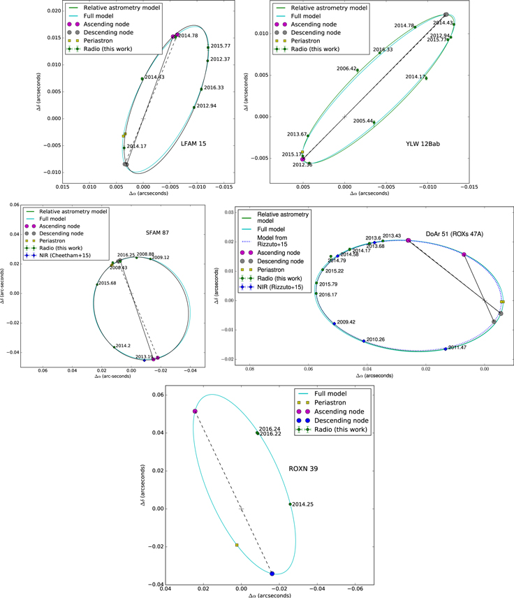
Figure 3. Relative positions of the components of the binary systems. The green points mark the detections with the VLBA, while blue points indicate the detections in the NIR by Cheetham et al. (2015) and Rizzuto et al. (2016). Green and cyan solid lines correspond to the "relative astrometry" and "full" model orbital fits, respectively. The blue dotted line in the fourth panel is the fit by Rizzuto et al. (2016) to NIR only data. The black solid and dashed lines trace the line of nodes of the "relative astrometry" and "full" model, respectively. The cross marks the position of the primary source.
Download figure:
Standard image High-resolution imageThe results from both fits are given in Table 6, and the resulting orbits are shown in Figure 3. We find that both fits are consistent with each other within the errors. We will comment on each system separately in the following subsections.
Table 6. Orbital Elements
| Name | a | P | T0 | e | Ω | i | ω | M1 | M2 | MT |
|---|---|---|---|---|---|---|---|---|---|---|
| (mas) | (years) | (°) | (°) | (°) | (M ) ) |
(M ) ) |
(M ) ) |
|||
| (1) | (2) | (3) | (4) | (5) | (6) | (7) | (8) | (9) | (10) | (11) |
| LFAM 15 | ||||||||||
| Full | 16.40 ± 0.13 | 3.591 ± 0.0183 | 2007.008 ± 0.039 | 0.528 ± 0.005 | 337.93 ± 0.81 | 110.30 ± 0.49 | 235.54 ± 1.02 | 0.4687 | 0.421 | 0.89 |
| ± 0.0146 | ± 0.010 | ± 0.01 | ||||||||
| Rel. astr. | 16.98 ± 0.16 | 3.598 ± 0.0099 | 2010.626 ± 0.011 | 0.561 ± 0.007 | 340.05 ± 0.49 | 109.77 ± 0.27 | 239.60 ± 0.64 | ⋯ | ⋯ | 0.99 |
| ± 0.03 | ||||||||||
| YLW 12Bab | ||||||||||
| Full | 12.70 ± 0.09 | 1.425 ± 0.0012 | 2005.174 ± 0.009 | 0.444 ± 0.003 | 135.15 ± 1.03 | 75.60 ± 1.25 | 158.69 ± 1.47 | 1.3969 | 1.258 | 2.66 |
| ± 0.0194 | ± 0.006 | ± 0.02 | ||||||||
| Rel. astr. | 12.54 ± 0.06 | 1.424 ± 0.0005 | 2013.720 ± 0.003 | 0.442 ± 0.003 | 135.38 ± 0.32 | 74.32 ± 0.48 | 160.11 ± 0.99 | ⋯ | ⋯ | 2.58 |
| ± 0.07 | ||||||||||
| SFAM 87 | ||||||||||
| Full | 35.58 ± 0.31 | 7.691 ± 0.007 | 2023.781 ± 0.006 | 0.343 ± 0.001 | 22.36 ± 8.57 | −162.66 ± 2.84 | 346.19 ± 8.83 | 1.0207 | 0.999 | 2.02 |
| ± 0.0224 | ± 0.038 | ± 0.04 | ||||||||
| Rel. astr. | 35.79 ± 0.30 | 7.719 ± 0.019 | 2008.404 ± 0.015 | 0.341 ± 0.005 | 18.62 ± 4.32 | −157.95 ± 2.59 | 344.25 ± 4.91 | ⋯ | ⋯ | 2.06 |
| ± 0.09 | ||||||||||
| DoAr 51 | ||||||||||
| Full | 32.83 ± 0.45 | 8.102 ± 0.063 | 2012.025 ± 0.044 | 0.802 ± 0.004 | 51.56 ± 6.31 | 18.95 ± 1.75 | 216.41 ± 6.42 | 0.7909 | 0.781 | 1.57 |
| ± 0.0140 | ± 0.042 | ± 0.05 | ||||||||
| Rel. astr. | 32.47 ± 0.39 | 8.070 ± 0.035 | 2012.020 ± 0.029 | 0.801 ± 0.005 | 51.81 ± 9.66 | 17.80 ± 4.36 | 215.81 ± 10.20 | ⋯ | ⋯ | 1.54 |
| ± 0.07 | ||||||||||
| Rizzuto+16 | 32.69 ± 0.35 | 8.233 ± 0.117 | 2012.009 ± 0.010 | 0.818 ± 0.009 | 24.1 ± 11.0 | 16.3 ± 2.0 | 243.0 ± 10.9 | ⋯ | ⋯ | 1.57 |
| ± 0.03( ± 0.29) | ||||||||||
| ROXN 39 | ||||||||||
| Full | 54.3 ± 3.9 | 11.2 ± 1.5 | 2056.1 ± 1.2 | 0.40 ± 0.12 | 25.4 ± 2.9 | 68.4 ± 3.3 | 120.0 ± 12.9 | 2.31 | 0.97 | 3.3 |
| ± 1.04 | ± 0.50 | ± 1.2 | ||||||||
| S1 | ||||||||||
| Full | 19.99 ± 0.20 | 1.734 ± 0.003 | 2017.089 ± 0.020 | 0.745 ± 0.010 | 118.9 ± 17.7 | 36.2 ± 6.1 | 294.6 ± 15.8 | 5.78 | 1.18 | 6.95 |
| ± 0.15 | ± 0.10 | ± 0.18 | ||||||||
Download table as: ASCIITypeset image
4.2.1. LFAM 15
The source LFAM 15 has been found to be double in 7 out of our 10 observed epochs. LFAM 15 was also observed in four epochs as part of project BL128 (Table 5), between 2005 June and 2006 March. We have calibrated these additional data and detected the source in three epochs, albeit always as a single component. In Figure 4, we show the measured positions for each component and the resulting best "full model" fit that, as mentioned before, consists of the sum of orbital motion around the center of mass, proper motion, and parallax of the system.

Figure 4. Observed positions and best fit for LFAM 15. Left: measured positions of each component are shown as red and blue circles. The solid lines show the fit corresponding to the "full model" described in the text. Middle: the squares mark the measured positions with the parallax signature removed, while the dashed lines are the fits from the "full model," also without parallax. Right: green dots mark the position of the center of mass derived using the solutions from the orbital model for the mass ratio. The green dashed line is the model for the motion of the center of mass of the system, while the red line is this same model with the parallax signature removed. The red squares indicate the position of the center of mass expected from the model without parallax. The arrow shows the direction of position change with time. Positional errors, as delivered by JMFIT, are smaller than the size of the symbols.
Download figure:
Standard image High-resolution image4.2.2. YLW 12B
YLW 12B is found to be a hierarchical triple source formed by a close binary (separation of 4–17 mas, equivalent to 0.6–2.4 au), detected in nine epochs, and a third component, located a few hundred mas to the southwest of the binary and detected in seven epochs (Figure 5). Hereafter, we call the close binary YLW 12Bab and the third component YLW 12Bc. Six archival VLBA observations, obtained between 2005 and 2006 as part of project BL128, have also been found for this source; they have been calibrated and analyzed (Table 5). One of these older epochs was discarded due to poor weather conditions during the observations. In these archival observations, both components of YLW 12Bab were detected on 2005 June 8 and 2006 June 1, while YLW 12Bc was detected on 2005 June 8 and 2006 March 24.
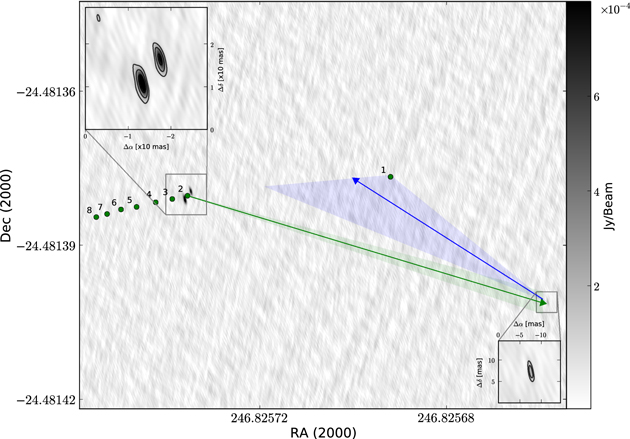
Figure 5. VLBA image of the multiple system YLW 12B, from data obtained on 2012 May 11 (first epoch observed by GOBELINS). Insets show zooms on the tight binary YLW 12Bab, top left, and the southwestern companion YLW 12Bc, bottom right. Contour levels are 3, 9, and 21 (in top left inset), and 3 and 5 (in bottom right inset) times  , the rms noise in the image. The green dots mark the position of YLW 12Bab relative to YLW 12Bc at the epochs when the three sources in the system are detected. These are eight epochs, which correspond to the Julian dates listed in Table 3 for the third component in the system as follows: 1 = 2453529.77467, 2 = 2456058.83738, 3 = 2456269.26236, etc. Notice that at the epoch with JD = 2453818.98287, the third component was detected but the compact binary was not. The arrows with their error cones show the acceleration vectors at the first epoch observed by GOBELINS.
Download figure:
Standard image High-resolution imageGiven the distance to the source, the angular separation between YLW 12Bab and YLW 12Bc of ∼140 and ∼320 mas in 2005 and 2016, respectively, corresponds to 20 to 45 au. This suggests that the sources form a bound multiple system, and later in this section we provide stronger evidence that supports this conclusion. To fit the positions of the YLW 12Bab components, and to take the effect of the third companion into account, we add two more free parameters to the "full model." These parameters are the acceleration of the center of mass of YLW 12Bab in each direction,  and
and  , which we consider to be uniform. As in the case of LFAM 15, three plots were constructed to visualize the best fit solution. In the first panel of Figure 6, we show the observed positions of the compact binary and the best fit, while in the second panel, we show this fit and source positions with the effect of parallax removed. Using the solution for the mass ratio from the "full model," we now compute the positions of the center of mass of YLW 12Bab, and plot them along with the parallax plus proper motion model in the third panel of Figure 6. It is clear that the compact binary follows a curved motion as a result of the gravitational force exerted by the third companion. Indeed, we find that the acceleration is statistically different from zero at
  in both directions.

Figure 6. First through third panels are like Figure 4, but for YLW 12Bab. The fourth panel shows the observed positions and best independent fit for YLW 12Bc, with parallax fixed to the value of YLW 12Bab.
Download figure:
Standard image High-resolution imageLet us now discuss the third star of the system. The positions of YLW 12Bab relative to YLW 12Bc, as well as the acceleration vector of YLW 12Bab, are shown in Figure 5. We see that the acceleration vector of YLW 12Bab points toward YLW 12Bc, as would be expected of a gravitationally bound system. This plot also shows that our assumption of a uniform accelerated motion is a reasonable approximation, because our observations cover only a small fraction of the orbit expected for the wider system. We attempted to fit the orbit of this source around the center of mass of the whole system with a simultaneous distance and proper motion fit for the three stars. However, we were not able to constrain most of the orbital parameters because the VLBA detections of the third companion are still insufficient. We only find solutions for the following parameters: Ω ∼ 85°, ϖ = 7.190 ± 0.088 mas,  mas yr−1,
  mas yr−1; limits on the mass,
  , period,
  , and that inclination is consistent with the compact binary. Even though we do not have enough data for modeling the orbit of YLW 12Bc, we can still constrain its proper motion and acceleration using its absolute positions measured with the VLBA. In order to do so, we fit the third star separately using the astrometric code for single sources to solve solely for proper motion and acceleration terms, while fixing the parallax at the value derived for YLW 12Bab. We show this last fit in the fourth panel of Figure 6, and give the solution of the astrometric parameters in Table 4.
As mentioned previously, the trajectory of YLW 12Bab is somewhat curved. That of YLW 12Bc is, on the other hand, more linear. This results in a smaller measured acceleration for YLW 12Bc (∼0.2 mas yr−2) than for YLW 12Bab (0.64 mas yr−2), and suggests that YLW 12Bc is the most massive member of the system. Indeed, we find that  , while
  and
and  . This is the reason why we plot the position of YLW 12Bab relative to YLW 12Bc in Figure 5, rather than the converse. We also see that, as expected, the acceleration of YLW 12Bc points, within the errors, toward YLW 12Bab (see Figure 5).
4.2.3. SFAM 87
SFAM 87 (also called ROX 39) has been detected in four epochs of GOBELINS. This source was also observed in six epochs from March 2008 to May 2009 as part of project BT097, but these data are yet to be published. We calibrated these additional epochs (Table 5) and combined them with our more recent data for the astrometric fits. The source is resolved into two components that are simultaneously detected in 6 out of the 10 total epochs (3 in BT097 and 3 in GOBELINS). We note that Cheetham et al. (2015) identified a companion to SFAM 87 in March 2013, using NIR aperture masking. This source appears to be the counterpart of the secondary source detected in our VLBA images (Figure 3). We used all available VLBA and NIR data to fit jointly orbital and proper motion, as well as parallax. The resulting best fit is shown in Figure 7 in a similar fashion to LFAM 15.

Figure 7. Same as Figure 4, but for SFAM 87.
Download figure:
Standard image High-resolution image4.2.4. DoAr 51
DoAr 51 (also called ROXs 47A) is located in the Lynds 1689 eastern streamer, 12 east of the Ophiuchus core. The source has been detected in seven epochs, and was found to be double in all of them. DoAr 51 was identified as a hierarchical triple system composed of a tight binary with separation of about 40 mas and a third component about 0.8 arcsec away by Barsony et al. (2003). Cheetham et al. (2015) confirmed the tight binary using NIR aperture masking observations. They resolved the source into two components, with an angular separation of 51.5 ± 0.20 mas in June 2009 and 43.38 ± 0.18 mas in April 2010. This is to be compared with a separation of 40 ± 30 mas reported by Barsony et al. (2003) in May 2002. More recently, Rizzuto et al. (2016) used the two positions measured by Cheetham et al. (2015) and three new detections in the NIR to model the orbit of the system. These five detections are shown in Figure 3, together with the positional offsets between the components of the system as seen in our VLBA images. It is clear that our radio sources are the counterparts of the NIR sources, as they lie along the orbit derived by Rizzuto et al. (2016). We model all data available from VLBA and NIR observations to better constrain the orbit of the system. The resulting best fit using the "full model" is shown in Figure 8, and the corresponding orbit in Figure 3. For comparison, we also show in this latter figure the orbit derived by Rizzuto et al. (2016).

Figure 8. Same as Figure 4, but for DOAR 51.
Download figure:
Standard image High-resolution image4.2.5. ROXN 39
The components of the system ROXN 39 have been detected separately in seven and five epochs, respectively, and simultaneously in only three epochs. The "full model" fit and measured positions of individual components are shown in Figure 9, while Figure 3 shows the same model and relative positions. We did not fit the "relative model" to this system because of the small number of simultaneous detections of both components. Consequently, the orbital parameters are less constrained, compared to the other systems described previously.

Figure 9. Same as Figure 4, but for ROXN 39.
Download figure:
Standard image High-resolution image4.2.6. S1
This source has been detected in a total of 8 epochs, and was also observed at 14 epochs as part of projects BL128 and BT093 (Table 5). The distance estimate by Loinard et al. (2008) of  pc, based on the data from the first six of these old epochs, is significantly different from the distance obtained here for others sources in Lynds 1688 (which range from 130 to 140 pc), and hence requires a careful inspection. We re-calibrated the data used in Loinard et al. (2008), as well as the additional eight unpublished observations obtained as part of BL128 and BT093. Similarly to DoAr 21, source positions measured at these 14 older epochs were corrected before fitting the data, by the positional offset of the calibrator, J1625-2527, relative to its old position.
A second source was detected in four epochs of the archival data, at an angular separation of about 20–30 mas from S1 (Figure 10). The detections are, however, only evident by self-calibrating the images, and the source is not present in the most recent epochs, so they should be taken somewhat cautiously. It is interesting, however, that Richichi et al. (1994) did report on the detection, using the lunar occultation technique in the NIR, of a companion to S1 at about 20 mas. Our detections of a second source in the system would be consistent with that earlier result. If we assume that the source is double, we can fit the orbital motion of the system jointly with the astrometric parameters and use the positions of the putative second component to estimate individual masses. To that end, we discard the BL128 and 2nd BT093 secondary epochs, as well as the second, fourth, and sixth BT093 primary epochs, because their corresponding images are of poor quality due to observing issues (cf. Table 5), and source positions do not match up to the best fit solution. The "full model" fit, shown in Figure 11, yields  mas and a distance of 138.0 ± 1.7 pc. The derived mass for the primary component is
  , which is consistent with its B4 spectral type, while for the secondary we find a mass of
  . When ignoring the secondary component, the purely astrometric fit to all available data of the primary source yields
  mas, and hence the distance derived by Loinard et al. (2008). It is clear that this discrepancy in the results from the astrometry alone and the "full model" fits is due to the fact that the former does not take into account the multiplicity of the source. In the rest of the paper, we will use the results based on the astrometric plus orbital model, which are consistent with the distances obtained for other sources in Lynds 1688. Since the two components are detected simultaneously in only two epochs, we are not able to fit the "relative model" to relative positions, and only provide the resulting orbital parameters from the "full model" in Table 6.

Figure 10. Two components of S1 detected on 2007 June 21 The contours are 4, 8, 16, and 32σ, where  μJy is the rms noise of the image.
Download figure:
Standard image High-resolution image
Figure 11. Same as Figure 4, but for S1.
Download figure:
Standard image High-resolution image4.2.7. VSSG 11
VSSG 11 has been detected in seven observed epochs, and was found to be double in the last three. The second component is separated about 9 mas from the primary source. We perform the fits similarly to the other multiple systems discussed previously. However, because our observations only cover a small fraction of the orbit, the "full model" fit to the secondary source does not converge. This produces considerably larger errors in the astrometric and orbital parameters than those derived for the other multiple systems. Also, we were not able to reproduce the observed separations between the components of the system. We then fit solely parallax and accelerated proper motion. The resulting best fit is shown in Figure 12.
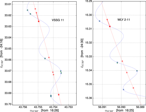
Figure 12. Same as Figure 2, but for VSSG 11 and WLY 2-11.
Download figure:
Standard image High-resolution image4.2.8. WLY 2-11
WLY2-11 has been detected in a total of five epochs. We resolve it into a double source in the last epoch, where the companion is detected at  . Since there are insufficient detections of primary and secondary for attempting to model the orbit, we can only fit one of the components of the system. We find that a good fit to the data is produced only when we discard the first epoch and consider for the fit the fainter component detected in the last epoch. If, instead, we take the positions of the single component as measured at the first four epochs and the position of the brightest component detected in the last observation, the fit does not match all the measured points, producing large errors in the astrometric parameters. Thus the detection at the first epoch probably corresponds to the companion source, which is detected as the brightest source in the last epoch. The fit, including acceleration terms, is shown in Figure 12. Because of the few detections, we are not able to estimate systematic errors on the source positions. Nevertheless, the derived parameter uncertainties are comparable to those from the fits that do incorporate systematic errors on source positions.
4.3. YLW 15
We have observed the Class I protostar YLW 15 at 11 epochs, and clear detections were obtained at five. Only one source is detected in the VLBA images, and since YLW 15 is known to be a binary system (Curiel et al. 2003), it is important to determine which of the two stars is detected in our VLBA data. This can be achieved by comparing the astrometry of the present VLBA observations with that of the VLA data published by Curiel et al. (2003), which were obtained between 1990 and 2002. Such a comparison is shown graphically in Figure 13. The positions of the two sources in the system (VLA 1 and VLA 2) are shown as a function of time as black and red symbols, respectively. We also calibrated and imaged the data from a VLA observation obtained in 2007 as part of project AF455. The VLBA positions are shown as blue symbols. It is clear that the source detected with the VLBA is located very near the expected position of VLA2 at the epochs of the VLBA observations, and more than half an arcsecond away from the expected position of VLA1. We conclude that the source detected with the VLBA is VLA2.
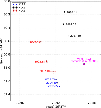
Figure 13. Observed positions of the components of YLW 15. Red and black circles mark positions measured with the VLA at the indicated epochs. The blue circles show the positions obtained from our VLBA observations. The triangle marks the position reported by Forbrich et al. (2007) from HSA observations.
Download figure:
Standard image High-resolution imageA marginal (7–9σ) VLBI detection of YLW 15 has been reported in the past (Forbrich et al. 2007). Indeed, the authors themselves mentioned that their detection was difficult to interpret, as the position did not coincide with the expected location of any of the two protostars in the system. This can also be seen in our Figure 13, where the position of the VLBI source reported by Forbrich et al. (2007) is shown as a cyan triangle. Their observations were conducted, under project code BF083, with the High Sensitivity Array (HSA), which for that run consisted of the Green Bank (GBT) 100 m radio telescope, the phased Very Large Array (equivalent in collecting area to a 130 m dish), as well as the VLBA. We calibrated these data following the standard procedures for incorporating non-VLBA antennas. We achieve rms noise levels between 10 and 22  (depending on the AIPS ROBUST parameter used for imaging), which are consistent with the value reported by Forbrich et al. (2007) of 15.4
  . We do not detect the source, and confirm our suspicion that their detection was likely spurious.
Even though five data points are, in principle, enough to perform an astrometric fit, most of our VLBA detections of YLW15 were obtained rather closely in time (two are separated by ∼3 weeks and other two by only ∼3 days). Moreover, the five detections were acquired around successive spring equinoxes, with no detection close to the fall equinox. As a result of this, the astrometric fit produces unreliable results. We will wait until we have more detections for the derivation of the astrometric parameters of this star.
5. THE DISTANCE TO OPHIUCHUS
In this paper, we report on 16 independent trigonometric parallax measurements. These results are listed in Table 4 and summarized graphically in Figure 14. They largely surpass all previously published distance measurements for Ophiuchus.
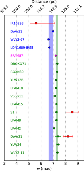
Figure 14. Summary of the parallax measurements reported here. Green circles and characters are for sources in the core (Lynds 1688), while blue circles and characters are for sources in the eastern streamer (Lynds 1689). SFAM 87 is shown with a different color because it lies neither within the core nor within the boundaries of Lynds 1689. The red squares are for previously published parallaxes (Imai et al. 2007; Loinard et al. 2008). The green vertical bar shows the mean parallax value for sources in the core, and its standard deviation (see text).
Download figure:
Standard image High-resolution imageOut of these 16 measurements, 12 are for YSOs in the Ophiuchus core (Lynds 1688). The parallaxes for these 12 sources are highly consistent (Figure 14) and yield a weighted mean value ϖ = 7.28 mas, with a weighted standard deviation  mas. In terms of distance, this corresponds to d = 137.3 pc, with a standard deviation
  pc. In principle, the standard deviation around the mean value could reflect both the uncertainties in our distance measurements, and the true depth of the complex. Since our uncertainties on individual parallax measurements are typically larger than 0.06 mas, we argue that the measured weighted standard deviation is completely dominated by the uncertainties on individual parallaxes rather than by the true depth of the core. We will, therefore, adopt this value as our final uncertainty on the distance to the core. We note that Lynds 1688 is about 075 across (Figure 15), corresponding to 1.8 pc. Thus our results indicate that it is not significantly more elongated along the line of sight than on the plane of the sky.

Figure 15. Spatial distribution of YSOs in Ophiuchus with astrometric parameters derived in this work. The gray scale represents the extinction map obtained as part of the COMPLETE project (Ridge et al. 2006), based on 2MASS data (Skrutskie et al. 2006). The gray contour indicates an AV of 4. The arrows correspond to the tangential velocity corrected by the solar motion.
Download figure:
Standard image High-resolution imageWe currently can only provide limited information on the location of the streamers relative to the core, since we only have measured parallaxes in the eastern streamer (Lynds 1689), and have just three independent measurements there (the parallaxes of LDN 1689 IRS 5, WLY 2-67, and DoAr 51). The weighted mean value of these three measurements is ϖ = 6.79 ± 0.16 mas, corresponding to d = 147.3 ± 3.4 pc. This suggests that the eastern streamer is about 10 pc farther than the core, although more parallax measurements of sources in Lynds 1689 would be required to confirm this. Interestingly, Imai et al. (2007) have measured the parallax of water masers in the protostar IRAS 16293-2422, located in the northern part of Lynds 1689, and found a value ϖ =  mas, which is consistent within 1 sigma with our parallax estimate for Lynds 1689 (Figure 14). Notice that we have not considered SFAM 87 in the previous analysis. It certainly lies somewhat outside of Lynds 1688 (Figure 15), and was considered as belonging to the Lynds 1689 "fringe" by McClure et al. (2010). These latter authors, however, do not explain how they arrived at such a conclusion, and we note that SFAM 87 does not formally lie within the boundaries of Lynds 1689. We find that its parallax is more consistent with the mean weighted parallax of the Ophiuchus core, suggesting that it is not part of Lynds 1689. This will also be confirmed when the distance to stars in the central parts of this cloud becomes available.
The typical distance to Ophiuchus that is generally used in the pre-main sequence literature is 125–130 pc. Our new distance is about 12% larger, which translates to a luminosity increase of  , and makes YSOs slightly younger with respect to evolutionary tracks.
Finally, we should mention that the stellar population of Ophiuchus could be contaminated by stars from the Upper Sco association, which is located at a similar distance (∼140 pc; de Zeeuw et al. 1999) and overlaps the Ophiuchus region in the sky. The YSOs in Ophiuchus show extinctions in the range  mag (Table 2), whereas the associated members of Upper Sco typically have
  mag (Walter et al. 1994). The fact that our detected YSOs have larger extinctions than Upper Sco ensures that these objects are part of the Ophiuchus Complex.
5.1. Proper Motions
Figure 15 shows the distribution of the 16 individual sources with astrometric parameters measured in this paper. In order to calculate the motion of each source relative to its local environment, we need to remove the contribution of the solar peculiar motion. For this correction, we use the formulation of Abad & Vieira (2005), and the solar motion relative to the LSR derived by Schönrich et al. (2010). They obtained rectangular components of the solar motion (u⊙, v⊙, w⊙) = (11.1 ± 0.7, 12.2 ± 0.47, 7.25 ± 0.37) km s−1, directed toward the Galactic center, the direction of Galactic rotation, and the Galactic north pole, respectively. Corrected proper motions were transformed to tangential velocities (Table 7) and overlaid on Figure 15. It is clear that, with the exception of a few objects that may belong to a different substructure of the complex, all sources share similar motions. The derived one-dimensional velocity dispersion in R.A. and decl. of sources in Lynds 1688 are 2.8 and  , respectively. These are larger than the values found in other studies, which range from ∼1 to 2 km s−1 (Makarov 2007; Wilking et al. 2015). However, our sample size is small, and our results need to be confirmed with additional proper motions and parallaxes. In addition, we estimate that the associated errors of the velocity dispersions (assumed to be Gaussian distributed) are 1.8 and 2.0 km s−1, in R.A. and decl., respectively. Thus, within the errors, our results are still consistent with past measurements.
Table 7. Corrected Proper Motions and Tangential Velocities
| Name |

|

|

|

|
|---|---|---|---|---|
| (mas yr−1) | (mas yr−1) | (km s−1) | (km s−1) | |
| (1) | (2) | (3) | (4) | (5) |
| WLY2-11 | −1.96 ± 0.72 | −4.2 ± 0.75 | −1.26 ± 0.46 | −2.72 ± 0.49 |
| YLW24 | 0.63 ± 0.83 | −4.17 ± 0.84 | 0.41 ± 0.53 | −2.67 ± 0.54 |
| DoAr21 | −11.74 ± 0.89 | −5.91 ± 0.86 | −7.54 ± 0.57 | −3.79 ± 0.55 |
| LFAM2 | 1.87 ± 0.87 | −6.94 ± 0.73 | 1.26 ± 0.58 | −4.66 ± 0.49 |
| LFAM8 | 1.82 ± 0.83 | −8.96 ± 0.76 | 1.19 ± 0.54 | −5.86 ± 0.5 |
| S1 | 5.65 ± 0.88 | −6.1 ± 0.77 | 3.69 ± 0.57 | −3.99 ± 0.51 |
| LFAM15 | 1.37 ± 0.74 | −6.29 ± 0.71 | 0.9 ± 0.49 | −4.11 ± 0.46 |
| VSSG11 | −2.88 ± 0.92 | −18.67 ± 0.9 | −1.9 ± 0.61 | −12.36 ± 0.59 |
| LFAM18 | −3.96 ± 0.82 | 2.25 ± 0.71 | −2.59 ± 0.53 | 1.47 ± 0.46 |
| YLW12B | 3.05 ± 0.77 | −3.66 ± 0.7 | 2.0 ± 0.5 | −2.4 ± 0.46 |
| ROXN39 | 0.33 ± 0.91 | −5.25 ± 0.83 | 0.21 ± 0.59 | −3.4 ± 0.54 |
| DROXO71 | 3.22 ± 0.81 | −7.77 ± 0.72 | 2.09 ± 0.52 | −5.03 ± 0.47 |
| SFAM87 | −0.41 ± 0.86 | −5.48 ± 0.76 | −0.27 ± 0.56 | −3.6 ± 0.5 |
| LIRS5 | 0.21 ± 0.71 | −3.55 ± 0.69 | 0.15 ± 0.5 | −2.52 ± 0.49 |
| WLY2-67 | 0.58 ± 0.79 | −5.06 ± 0.67 | 0.41 ± 0.57 | −3.63 ± 0.48 |
| DoAr51 | 2.1 ± 0.84 | −3.15 ± 0.72 | 1.43 ± 0.57 | −2.14 ± 0.49 |
Download table as: ASCIITypeset image
6. SUMMARY
We have presented the first results from GOBELINS toward the region of Ophiuchus. We observed a total of 50 YSOs with the VLBA, and detected 26 of them. Most of our VLBA-detected YSOs are Class II-III, but three Class I sources have also been detected. The YSOs detected here are clearly non-thermal emitters (otherwise they would not be detected with the VLBA), so our observations have revealed the existence of a large population of non-thermal YSOs in Ophiuchus. About 30% of our the VLBA-detected YSOs belong to tight multiple systems with angular separations from 0.6 to 44 au. While this fraction appears to be consistent with the binarity fraction in Ophiuchus measured in a recent infrared multiplicity survey, we note that most of the binaries detected with the VLBA are very tight systems with separations below 10 au.
The astrometry of 16 young stellar systems was presented. Absolute positions of single sources were modelled to derive parallaxes and proper motions, and source distances were then obtained with a few percent accuracy. For sources in multiple systems, we use individual positions and, in most cases, angular separations to model jointly orbital and astrometric parameters. For these sources, the distance was measured with 0.3%–2% accuracy. Because the VLBA delivers absolute positions for each component, we were able to determine the individual masses in six of the eight total multiple systems; masses range from ∼1 to 7  .
.
Twelve sources are associated with the Ophiuchus core (Lynds 1688). They yield a mean distance of 137.3 ± 1.2 pc, and no indication of a detectable depth. Three sources for which the astrometric elements could be measured are located in the eastern streamer (Lynds 1689); the measurements imply a distance of 147.3 ± 3.4 pc for this cloud. This result suggests that the eastern streamer is 10 pc more distant than the core, but this needs to be confirmed when more parallaxes become available.
The measured proper motions of young stars in the core yield one-dimensional velocity dispersions in R.A. and decl. of 2.8 ± 1.8 and 3.0 ± 2.0 km s−1, respectively. This result may indicate that our sources belong to different substructures of the complex. However, our result may suffer from small-number statistics, and the associated errors are large. Indeed, our values are consistent within  with velocity dispersions of
  , which have been measured in the past.
Finally, we note that six YSOs have been detected only two or three times with the VLBA in the observations presented here. For these sources, no meaningful astrometric fit could yet be performed, but this will become possible once a few additional detections are obtained in the coming few years. Thus we anticipate that we will soon be able to increase the number of individual trigonometric parallaxes in Ophiuchus.
G.N.O.-L., L.L., L.F.R., R.A.G.-L., G.P., and J.L.R. acknowledge CONACyT, Mexico, for financial support through grants 339802, 104497, 153522, and I0017-151671. L.L. and R.A.G.-L. were supported by DGAPA, UNAM grant PAPIIT IG100913. L.L. and G.N.O.-L. also acknowledge support from the von Humboldt Stiftung. N.J.E. was supported by NSF grant AST-1109116 to the University of Texas at Austin. P.A.B.G. acknowledges financial support from FAPESP. The National Radio Astronomy Observatory is operated by Associated Universities, Inc., under cooperative agreement with the National Science Foundation. This work made use of the Swinburne University of Technology software correlator, developed as part of the Australian Major National Research Facilities Programme and operated under licence.
APPENDIX A: NON-THERMAL RADIO EMISSION IN YOUNG STARS AND GOBELINS DETECTION STATISTICS
A.1. Introduction
YSOs are often detectable radio sources due to a variety of mechanisms. One common radio emission process in YSOs is thermal bremsstrahlung (free–free) continuum emission, either from photo-ionized gas around massive stars (e.g., Churchwell 2002) or from shock-ionized gas in supersonic jets and outflows (e.g., Rodríguez 1997). The brightness temperature corresponding to thermal bremsstrahlung emission, however, is typically only 104 K—much too small to be detectable in VLBI observations. The situation with thermal dust continuum emission, which can be detected up to centimeter wavelengths from circumstellar disks (e.g., Pérez et al. 2015), is even worse, as such emission has brightness temperatures of at most several hundred K. Thermal line emission, from molecules or atoms, is similarly limited to brightness temperatures smaller than several hundred K. Thus to find emission that could be detected in VLBI observations, one must turn to non-thermal mechanisms. For line emission, this implies focusing on strongly amplified maser lines, like those of water (H2O), methanol (CH3OH), formaldehyde (H2CO), silicon monoxide (SiO), or hydroxyl (OH). Those lines (particularly those of water and methanol) are widespread in regions of high-mass star formation, and can be detected and studied with VLBI observations up to distances of several kpc. Indeed, the BeSSeL project (Brunthaler et al. 2009) takes advantage of these lines to measure the parallax and proper motions of high-mass star-forming regions distributed across the entire Milky Way disk. In the Gould's Belt star-forming regions, however, only a handful of maser sources are known (e.g., Moscadelli et al. 2006).
Non-thermal continuum emission also exists, and broadly corresponds to the situation where electrons gyrate in a magnetic field. This type of radiation is called cyclotron, gyro-synchrotron, or synchrotron emission, depending on whether the electrons are non-relativistic (with a γ Lorentz factor of about 1), mildly relativistic (γ of a few), or ultra-relativistic (γ ≫ 1), respectively (Dulk 1985). Such continuum non-thermal emission has been detected around a number of low-mass young stars (e.g., Forbrich et al. 2011, and references therein), and has been interpreted as coronal emission from active stellar magnetospheres. The most common mechanism appears to be gyro-synchrotron, although maser-amplified cyclotron emission (Smith et al. 2003) as well as synchrotron emission (Massi et al. 2006) have also been reported in rare instances. The magnetic field in which the electrons are gyrating is generated through the dynamo mechanism, which requires convection in the outer layers of the stellar interior (e.g., Dormy et al. 2013). As a consequence, non-thermal coronal emission should occur only in low-mass stars, because intermediate and high-mass stars are fully radiative. This is true both for main sequence and pre-main sequence stars: while low-mass T Tauri stars approach the main sequence on fully convective Hayashi tracks, stars more massive than about 3  follow radiative Henyey tracks (e.g., Palla & Stahler 1993). It is noteworthy, however, that a few intermediate-mass young stars have been found to exhibit non-thermal coronal emission (Andre et al. 1991; Dzib et al. 2010). The electrons gyrating in the magnetic field are thought to be accelerated to mildly relativistic speeds during energetic reconnection processes (Parker 1957), so the emission is often produced in flares (e.g., Bower et al. 2003) and is therefore highly variable. Once again, there are some exceptions to this general behavior (e.g., Andre et al. 1991). Finally, it should be mentioned that most of the low-mass young stars where non-thermal emission has been reported are T Tauri stars (particularly Weak Line T Tauri stars), although a few younger Class I protostars have also been detected (Forbrich et al. 2006; Deller et al. 2013).
Coronal non-thermal radio continuum emission usually remains unresolved at the milli-arcsecond resolution of VLBI observations (e.g., Loinard et al. 2007; but see Andre et al. 1991). Theoretically, the emission is expected to be confined to the magnetosphere of the YSO, which extends to only a few stellar radii (Bouvier et al. 2007). This is indeed very small—for instance, 10  corresponds to about 0.5 mas at 100 pc.
A.2. Statistics
As mentioned in the main text, we have firmly detected a total of 26 YSOs, corresponding to roughly half of the 50 YSOs targeted in our observations. This confirms the claim by Dzib et al. (2013) that about 50% of the radio-bright YSOs in Ophiuchus are non-thermal emitters. We searched the literature and found that only six of these YSOs had previously been detected in VLBI experiments. These sources (DoAr 21, S1, LFAM 15, VSSG 11, YLW 12 B, and SFAM 87) were known to be magnetically active stars, with centimetric non-thermal radio emission, before our observations (e.g. Andre et al. 1992; Loinard et al. 2008). We note that Forbrich et al. (2007) reported on the detection, with the HSA, of one of the components of the binary class 0/I source YLW 15 (a target that we also detect here). However, our analysis of the proper motions of the system components (see Section 4.3) suggests that the detection by Forbrich et al. (2007) was likely spurious. The 26 detected YSOs correspond to a total of 34 individual young stars, because five detections are found to be tight binary systems, while one corresponds to a triple system (see Table 2).
Dzib et al. (2013) also published a list of YSOc detected in their VLA observations. They reported as YSOc those radio sources that are not associated with known young stars, but that show high VLA flux variations, a negative spectral index, or circular polarization. Four of these sources were also detected in our VLBA observations, as well as another 27 (presumably background) sources. We analyze the astrometry of these 31 objects in Appendix B and find that, as expected, most of them are extragalactic sources.
In order to establish the nature of the emission, we have measured the brightness temperature (Tb) of the VLBA-detected sources, according to

where  and
and  are the deconvolved sizes of the major and minor axes diameter, and
  is the total flux density measured in the VLBA images. Since most of the sources have been detected at several epochs, we are reporting the highest measured brightness temperature. For unresolved sources, we give a lower limit to Tb obtained using the corresponding beam size as an upper limit for the source size. Brightness temperatures are given in columns (7) and (5) of Tables 2 and 8, respectively. All of the VLBA-detected YSOs have
  K, which is larger than the brightness temperature expected for thermal bremsstrahlung radiation (
 K), and consistent with the brightness temperature expected for non-thermal emission. Our study has, therefore, found a population of non-thermal YSOs larger than previously reported. It is noteworthy that non-thermal emission is detected in sources in the Class I to Class III stages.
Table 8. Other Detected Sources
| GBS-VLA | Other Identifier | Maximum Flux | Maximum Flux | log [Tb (K)] | Type of Sourcea | Number of | |
|---|---|---|---|---|---|---|---|
| Name | at 5 GHz (mJy) | at 8 GHz (mJy) | Detections/Observations | ||||
| (1) | (2) | (3) | (4) | (5) | (6) | (7) | |
| J162540.94-244147.2 | SSTc2d J162540.9-244147 | 0.39 | <0.06 | 0.08 | E | ? | 1/1 |
| J162547.68-243735.7 | ⋯ | 0.45 | 0.37 | 0.05 | ? | E | 3/3 |
| J162633.48-241215.9 | SFAM12 | 0.39 | <0.06 | 0.05 | E | G | 2/2 |
| J162635.33-242405.2 | LFAM13 | 0.79 | <0.09 | 0.07 | E | E | 4/10 |
| J162646.36-242002.0 | LFAM17 | 0.64 | <0.06 | 0.08 | YSOc | G | 5/6 |
| J162702.15-241927.8 | GDS J162702.1-241928 | 0.48 | <0.06 | 0.07 | E | E | 4/4 |
| J162713.06-241817.0 | ⋯ | 0.21 | <0.06 | 0.05 | ? | E | 2/9 |
| J162718.25-243334.8 | ⋯ | 0.52 | <0.06 | 0.16 | ? | ? | 1/6 |
| J162729.23-241755.3 | ROC25 | 2.74 | <0.18 | 0.06 | E | E | 5/5 |
| J162734.55-242020.7 | ROC26 | 1.25 | <0.18 | 0.06 | E | E | 5/5 |
| J163027.69-243300.2 | SSTc2d J163027.7-243300 | 0.25 | <0.06 | 0.05 | E | E | 2/4 |
| J163032.26-243127.9 | SSTc2d J163032.3-243128 | 0.90 | <0.06 | 0.06 | YSOc | E | 3/3 |
| J163033.26-243038.7 | SSTc2d J163033.2-243039 | 0.40 | <0.06 | 0.06 | YSOc | ? | 1/3 |
| J163036.26-243135.3 | ⋯ | 0.80 | <0.06 | 0.07 | ? | E | 3/3 |
| J163109.79-243008.4 | ROC49 | 0.73 | <0.06 | 0.07 | E | E | 3/3 |
| J163115.25-243313.8 | ⋯ | 0.29 | <0.06 | 0.04 | ? | E | 2/4 |
| J163120.14-242928.5 | ROC52 | 4.38 | <0.06 | 0.14 | E | E | 3/3 |
| J163130.62-243351.6 | SSTc2d J163130.6-243352 | 0.64 | <0.06 | 0.06 | E | E | 3/3 |
| J163138.57-253220.0 | ⋯ | 0.56 | 1.00 | 0.07 | ? | G? | 4/4 |
| J163151.93-245617.4 | ⋯ | 0.34 | 0.28 | 0.06 | YSOc | Oph | 3/4 |
| J163154.49-245217.1 | SSTc2d J163154.5-245217 | 0.35 | <0.06 | 0.05 | E | E | 2/3 |
| J163159.36-245639.7 | SFAM127 | 1.72 | <0.06 | 0.09 | E | E | 2/2 |
| J163202.39-245710.0 | ⋯ | 0.18 | 0.34 | 0.06 | ? | E | 2/3 |
| J163210.77-243827.6 | SFAM130 | 0.42 | <0.09 | 0.07 | E | E | 4/5 |
| J163211.08-243651.1 | SSTc2d J163211.1−243651 | 0.80 | <0.09 | 0.08 | E | E | 5/5 |
| J163212.25-243643.7 | ⋯ | 0.37 | <0.06 | 0.07 | ? | E | 2/5 |
| J163213.92-244407.8 | ⋯ | 0.36 | <0.05 | 0.06 | ? | ? | 1/6 |
| J163227.41-243951.4 | SSTc2d J163227.4−243951 | 0.51 | <0.06 | 0.06 | E | E | 3/5 |
| J163231.17-244014.6 | SSTc2d J163231.2−244014 | 0.51 | <0.06 | 0.05 | E | E | 2/5 |
| J163245.23-243647.4 | SFAM200 | 0.47 | 0.26 | 0.07 | E | E | 3/3 |
| J163617.50-242555.4 | SFAM212 | 1.82 | 2.50 | 0.09 | E | E | 5/5 |
Note. Reported sources have flux densities greater than  and
and  in the cases of one or several detections, respectively. Non-detections are indicated by giving an upper flux density limit of
  .
.
Download table as: ASCIITypeset image
A.3. Non-thermal Emission as a Function of Evolutionary Stage and Multiplicity
In Figure 16, we plot the VLBA flux density at 5 GHz of the detected YSOs as a function of their evolutionary phase, as measured from their infrared/millimeter spectral energy distribution (SED). It appears at first glance that older objects have, on average, stronger non-thermal radio emission. The significance of this correlation can be assessed by a Kolmogorov-Smirnov test on the three YSOs classes. The p values derived from such a test are  , so we cannot reject the null hypothesis that different classes are taken from the same distribution function. The relation is, therefore, not statistically significant. We also perform the Wilcoxon rank-sum statistic finding similar results. Thus our conclusion about the significance of the correlation does not depend on the statistical test that we use.
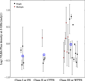
Figure 16. VLBA flux density at 5 GHz, as a function of evolutionary phase. The error bars represent the range in flux density from the maximum to the minimum measured values for variable sources, and measured flux uncertainties for sources with constant flux. Black circles correspond to single sources, while red triangles correspond to multiple systems. We adopt for the VLBA flux density of multiple systems the sum of the flux densities of individual components. The black points are the mean VLBA flux density for each individual object, whereas the open blue squares are mean values for each object type. Here and in the rest of the paper, FS stands for flat spectrum, CTTS for classical T Tauri, and WTTS for weak-lined T Tauri.
Download figure:
Standard image High-resolution imageFrom Table 2, it is clear that Class II and III sources are the most common types of YSOs with non-thermal radio emission. Past studies had only found two cases of Class I protostars with non-thermal emission detectable in VLBI observations. These sources are CrA IRS 5 (Deller et al. 2013) and EC 95 (Dzib et al. 2010). Here we have detected non-thermal emission from three other Class I objects, namely LFAM 4, YLW 15,20
and WLY 2-67. Therefore we have more than doubled the number of protostars with confirmed non-thermal emission. In a recent study, Heiderman & Evans (2015) investigated whether the Class 0+I and Flat SED sources identified in the c2d (Evans et al. 2009) and Gould Belt (Dunham et al. 2015) surveys are in the embedded phase. These authors used the detection of the  as a good indicator of the Stage 0+1, which corresponds to "a star and a disk embedded in a dense, infalling envelope" (van Kempen et al. 2009). Our three Class I objects with non-thermal radio emission meet the criterion to be in this embedded stage. Non-thermal emission has not been detected in Class 0 sources, and at this point it is unclear if this results from a lack of such emission or if such young systems always contain thermal radio jets that systematically absorb underlying active coronas.
Magnetic activity is known to occur throughout the early evolution of low-mass stars, so protostellar sources could easily produce non-thermal emission. On the other hand, accretion and outflow activity is also present in this protostellar stage. In order for the observer to see the radio emission from the stellar corona, the line of sight cannot cross regions where optically thick radio emission is present (i.e., the central portions of disks or wind/outflow systems). This might occur only for some privileged relative orientation of the system, and naturally explains the low fraction of detected protostars in our observations, in comparison with the larger number of detections of more evolved objects.
There does seem to exist a correlation between non-thermal radio emission in YSOs and multiplicity. Perhaps the best documented case is that of the V773 Tau system (Massi et al. 2002; Torres et al. 2012), where the radio flux increases by more than one order of magnitude when the system passes periastron. We have found here that a significant fraction of the VLBA-detected young stars belong to very tight binary or multiple systems (with a separation of a few tens of mas—a few au; Table 2). Multiplicity may help clear out the surrounding material, and result in non-thermal emission that is statistically less affected by free–free absorption, but the exact mechanisms behind this remain unclear. The flux from thermal jets becomes transparent at frequencies above a few GHz (Reynolds 1986). Thus coronal non-thermal emission from protostars with thermal emission should be detectable at higher frequencies.
In our VLBA observations, we found that seven YSOs form multiple systems, and one more has evidence of multiplicity (see Table 2). This represents  of the total number of YSOs detected with the VLBA. The angular separations of the components in these systems range from 4 to 315 mas, corresponding to 0.6–44 au at the distance of Ophiuchus. In order to investigate if this fraction is expected from the known population of multiple systems in Ophiuchus, or if it indicates that tight multiple systems are more likely to be non-thermal radio emitters than single stars or wider multiple systems, we compared it with the binary fraction reported in the literature. Recently, Cheetham et al. (2015) compiled high-resolution multiplicity data and combined them with their results from an aperture masking survey; they obtained a binary fraction of 35 ± 6% for spatial scales from 1.3 to 41.6 au. Taken at face value, our VLBA detection of 30% of binaries with separations between 0.6 and 44 au appears to be consistent with the binary fraction derived from the multiplicity survey by Cheetham et al. (2015). However, we still favor the idea that very tight binaries are more often radio sources than single stars or more separated binary systems, because seven of our eight detected binaries have separations of a few au, whereas only one has a separation larger than 10 au. Thus, for separations below 10 au, there does appear to be an excess of radio-bright binaries. Our interpretation will be tested by considering the whole sample of multiple stars seen in the five regions observed by GOBELINS, and comparing with multiplicity studies in the infrared, where aperture masking observations can explore angular separations similar to those attained with the VLBA.
A.4. Radio Luminosity Function of Non-thermal YSOs
We show in Figure 17 the number of objects versus the radio luminosity at 5 GHz (i.e., the luminosity function) of the 26 YSOs detected with the VLBA. The number of objects appears to decrease with increasing luminosity, following roughly a linear trend (in logarithmic luminosity). Assuming that the trend is valid for lower luminosities, we can infer that deeper observations with an improved sensitivity by an order of magnitude will detect ∼20 more YSOs with non-thermal radio emission, thus doubling the number of sources). It will be interesting to construct the luminosity function for the other regions considered in GOBELINS and see if this is a general trend.
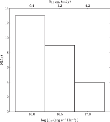
Figure 17. Luminosity function for the YSOs detected with the VLBA at 5 GHz.
Download figure:
Standard image High-resolution imageAPPENDIX B: OTHER SOURCES
In this section, we analyze the astrometry of 27 sources detected in our VLBA observations that are not classified as YSOs in the literature. These sources are listed in Table 8. Column (6) in that table provides a proposed classification based on the radio emission properties in the VLA observations of Dzib et al. (2013). Out of the 31 sources that are not known YSOs in that list, 18 are proposed to be extragalactic (E), 4 are YSO candidates (YSOc), and 9 have no proposed identifications. Many of these sources have been detected in several of our VLBA observations, so we can analyze their changes in position as a function of time to constrain their location along the line of sight. Extragalactic sources are expected to remain practically fixed on the celestial sphere, so any measured change in their positions should be of the order of or less than the rms astrometric errors. These errors are given by the systematic errors found in the astrometric fits and are  mas for YSOs in the core, while for sources located in the L1689 streamer, we obtain systematic errors
  mas. These larger errors in L1689 result from the larger separation between the main phase calibrator and the targets there. Galactic sources, on other hand, should show an appreciable parallax and a proper motion signature, particularly if they are within a few kpc.
For each source in Table 8 that has been observed in at least two epochs (i.e., 56 out of the 64 sources in Table 8), we measured the shift in position ( ) between consecutive epochs, normalized it to 1 year, and averaged over all consecutive pairs of epochs. For instance, for a source with three detections, we averaged two displacements: one between epoch 1 and epoch 2, and the other between epoch 2 and epoch 3. We will call this quantity the position change rate in the rest of this section. This position change rate should be zero (within the errors) for extragalactic sources and non-zero for (nearby) Galactic objects. However, since the position change rate contains information on both the parallax and the proper motions, and is based on a varying number of detections for different sources (from two to five detections), a non-zero value cannot be easily interpreted in terms of distance along the line of sight. Sources for which a non-zero value is found should be analyzed in more detail.
The results are shown in the form of a histogram in Figure 18, where we separate known YSOs from other sources. The two histograms are markedly different. For known YSOs, the histogram is roughly Gaussian and centered around a position change rate of ∼36 mas yr−1. For the rest of the sources, on the other hand, the distribution is dominated by a peak around a position change rate of zero, to within a few mas yr−1. Specifically, the first four bins in the histogram (23 sources) correspond to sources that do not show appreciable motion on the celestial sphere (i.e., they have position changes between consecutive epochs smaller on average than the astrometric noise), and we identify them as extragalactic. This new classification is shown in column (6) of Table 2. Of course, for the four unclassified sources that have only been detected once in our VLBA observations, the position change rate cannot be measured, and we classify these sources as "?" in column (6) of Table 8.
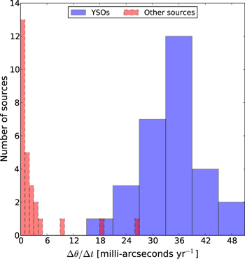
Figure 18. Histogram of the position change rate for all sources detected at least twice toward Ophiuchus. The sources previously identified as YSOs are shown in blue, whereas the other sources are shown in red.
Download figure:
Standard image High-resolution image
There are three sources, however, that do show a non-zero position change rate, and we now discuss these in turn. The source with the largest position change rate (∼27 mas yr−1) is GBS-VLA J163151.93-245617.4, and has been detected three times. However, as in the case of YLW15, the three detections occurred around the spring equinoxes. Thus it is impossible to obtain any meaningful information on its parallax. We note, however, that its position change rate places it squarely within the range covered by the YSOs in Ophiuchus. In addition, because the detections occurred only during spring equinoxes (April 2013, March 2014, and March 2016), the displacement is dominated by proper motions, with only a small contribution from parallax. The fact that the measured displacement (∼27 mas yr−1) is so similar to the proper motion of sources in Ophiuchus suggests that GBS-VLA J163151.93-245617.4 is not only Galactic but indeed an Ophiuchus member. Interestingly, this source had been classified as a YSO candidate by Dzib et al. (2013) on the basis of the variability and spectral slope of the radio emission. Additional detections will be necessary to confirm this and obtain a trigonometric parallax, but for the time being, we classify GBS-VLA J163151.93-245617.4 as an "Oph" member in column (6) of Table 8.
The source with the second largest position change rate (∼19 mas yr−1) is SFAM12, which was detected only twice. In this case, the two detections occurred around the spring equinox of 2015 and the fall equinox of 2015, respectively. Thus the displacement results from the combination of both parallax and proper motion. This makes it unlikely that SFAM12 is an Ophiuchus member, since for sources in Ophiuchus, a larger position change rate would be expected (roughly 25 mas yr−1 due to proper motion, and an additional 15 mas due to parallax, since the observations were obtained at opposite equinoxes). Thus we classify SFAM12 as a Galactic source ("G" in column (6) of Table 2), but unlikely to be associated with Ophiuchus itself. We note that SFAM12 was previously believed to be extragalactic. Finally, the third source with a definite non-zero position change rate (∼10 mas yr−1) is LFAM17. Since there were five detections of this target, an astrometric fit could be attempted. Formally, it suggests a parallax ϖ = 0.87 ± 0.14 mas (corresponding to d = 1.2 ± 0.2 kpc), but the fit is poor. Yet certainly this source is Galactic but much farther away than Ophiuchus. Thus we classify it as "G" in column (6) of Table 2. We note that Dzib et al. (2013) had classified it as a YSO on the basis of its radio properties. Both SFAM12 and LFAM17 are likely to be active stars (possibly, but not necessarily, young ones) located behind Ophiuchus.
To finish this section, we should mention source GBS-VLA J163138.57-253220.0, which is the sole member of the fifth red histogram bin in Figure 18. Its position change rate is formally above the astrometric uncertainty. It was detected four times, so an astrometric fit could again be attempted. As in the case of LFAM17, the fit is poor; it results in a parallax ϖ = 0.17 ± 0.05 mas (corresponding to d =  kpc). This might suggest that GBS-VLA J163138.57-253220.0 is a Galactic source at several kpc, but given the large errors and poor quality of the fit, we cannot completely discard that it be extragalactic. Thus we classify it as "G?" in column (6) of Table 8. In general, the identification proposed by Dzib et al. (2013) for sources in Table 8 matches well with our new classification based on VLBA observations.
Footnotes
- 17
VLBI arrays are equivalent to telescopes thousands of kilometers in diameter in terms of angular resolution, but emphatically not in terms of collecting area.
- 18
A French word referencing the tapestries designed by the Gobelin Manufactory in Paris, France.
- 19
This package is available at http://www.astro.gsu.edu/~gudehus/binary.html.
- 20