


ABSTRACT
A microlensing survey by Sumi et al. exhibits an overabundance of short-timescale events (STEs; tE < 2 days) relative to what is expected from known stellar populations and a smooth power-law extrapolation down to the brown dwarf regime. This excess has been interpreted as a population of approximately Jupiter-mass objects that outnumber main-sequence stars nearly twofold; however the microlensing data alone cannot distinguish between events due to wide-separation (a ≳ 10 au) and free-floating planets. Assuming these STEs are indeed due to planetary-mass objects, we aim to constrain the fraction of these events that can be explained by bound but wide-separation planets. We fit the observed timescale distribution with a lens mass function comprised of brown dwarfs, main-sequence stars, and stellar remnants, finding and thus corroborating the initial identification of an excess of STEs. We then include a population of bound planets that are expected not to show signatures of the primary lens (host) in their microlensing light curves and that are also consistent with results from representative microlensing, radial velocity, and direct imaging surveys. We find that bound planets alone cannot explain the entire STE excess without violating the constraints from the surveys we consider and thus some fraction of these events must be due to free-floating planets, if our model for bound planets holds. We estimate a median fraction of STEs due to free-floating planets to be f = 0.67 (0.23 ≤ f ≤ 0.85 at 95% confidence) when assuming "hot-start" planet evolutionary models and f = 0.58 (0.14 ≤ f ≤ 0.83 at 95% confidence) for "cold-start" models. Assuming a delta-function distribution of free-floating planets of mass  yields a number of free-floating planets per main-sequence star of N = 1.4 (0.48 ≤ N ≤ 1.8 at 95% confidence) in the "hot-start" case and N = 1.2 (0.29 ≤ N ≤ 1.8 at 95% confidence) in the "cold-start" case.
Export citation and abstract BibTeX RIS
1. INTRODUCTION
Deep optical and near-infrared photometric surveys to characterize the low-mass end of the substellar initial mass function (IMF) have identified populations of isolated, planetary-mass candidates in several nearby, young star-forming regions and clusters (Comeron et al. 1993; Itoh et al. 1996; Nordh et al. 1996; Tamura et al. 1998; Lucas & Roche 2000; Zapatero Osorio et al. 2000, 2002; McGovern et al. 2004; Kirkpatrick et al. 2006; Luhman et al. 2006; Bihain et al. 2009; Burgess et al. 2009; Scholz et al. 2009, 2012a, 2012b; Weights et al. 2009; Marsh et al. 2010; Quanz et al. 2010; Mužić et al. 2011, 2012, 2014, 2015). While a number of these photometrically identified candidates have met with some controversy in the literature concerning their youth (and thus low masses) or cluster membership (see e.g., Hillenbrand & Carpenter 2000; Allers et al. 2007; Luhman et al. 2007a, 2016), recent studies, in particular those by the Substellar Objects in Nearby Young Clusters (SONYC) group, have focused on obtaining confirmation spectra of such candidates and have verified several free-floating, planetary-mass objects with masses as low as a few Jupiter masses (Scholz et al. 2009, 2012a, 2012b; Mužić et al. 2011, 2012, 2015). Others have shown that in some cases, youth and cluster membership can be validated through the use of control fields outside of (yet near) open clusters (Peña Ramírez et al. 2012). Sumi et al. (2011) also presented evidence for a large population of ∼Jupiter-mass objects that are either wide-separation (a ≳ 10 au) or free-floating planets inferred from an excess of short events in the observed timescale distribution of a sample of microlensing events collected by the second phase of the Microlensing Observations in Astrophysics group (MOA-II; Sumi et al. 2003; Sako et al. 2008). Wyrzykowski et al. (2015) report that data from the third phase of the Optical Gravitational Lensing Experiment (OGLE-III; Udalski 2003) show a flattening in the slope of the observed event timescale distribution toward shorter timescales that is suggestive of a population of lenses similar to that reported by Sumi et al. (2011), although this flattening is only marginally significant due to uncertainties resulting from small-number statistics and a low detection efficiency to such short-timescale events.
Comparing the occurrence rates of free-floating planets inferred by imaging surveys with those from microlensing is difficult, as the imaging surveys have sensitivities that cut off around 1–3 MJup (and depend on the exact evolutionary model adopted), while Sumi et al. (2011) found that these objects (regardless of their boundedness) most likely have masses near (and probably below) the sensitivity limit of the imaging surveys at  . Nevertheless, in the SONYC survey of the young cluster NGC 1333, Scholz et al. (2012b) find that the occurrence rate of (photometrically identified, spectroscopically confirmed) free-floating, planetary-mass objects relative to main-sequence stars is smaller than that inferred by the Sumi et al. (2011) microlensing study by a very large factor of some 20–50. Scholz et al. (2012b) argue that the star formation process extends into the planetary-mass regime, down to the planetary masses they are able to probe, and thus this large difference in inferred occurrence rates of free-floating planets must be due to a very large upturn in the mass function of compact objects below ∼3 MJup that is perhaps indicative of a different formation channel (assuming that microlensing and direct imaging surveys are probing an analogous population of compact objects). Alternatively, one might argue that young open clusters may have a different mass function than the objects in the Galactic disk and bulge that give rise to microlensing events.
On the other hand, the photometric survey of ρ Oph by Marsh et al. (2010) finds a much larger number of isolated, planetary-mass objects per main-sequence star. After integrating their inferred mass function (shown in their Figure 8) in the planetary regime, the lowest two bins between 7 × 10⁻⁴ ≲ M/M⊙ ≲ 6 × 10⁻³ (corresponding to roughly  ), and in the stellar regime, the highest three bins between 0.08 ≲ M/M⊙ ≲ 1.0, we divide these values to estimate the implied number of free-floating planets per main-sequence star of ∼30. This number is over an order of magnitude larger than that of Sumi et al. (2011) and larger than the results of Scholz et al. (2012b) by an even greater factor. This seems to suggest that either the formation of free-floating planets is extremely sensitive to the local environment, the Marsh et al. (2010) sample is contaminated (with background stars or due to mis-estimates of the ages and/or masses of the candidate free-floating planets; see e.g., Luhman et al. 2007a and Allers et al. 2007) since they lack spectroscopic validation for many of their candidates, or some combination thereof.
Broadly, there are two formation channels for free-floating planets, but there are issues with the theory and observations behind each. The first, as Scholz et al. (2012b) claim, is that these objects form as an extension of the star formation process; however the lower mass fragmentation limit predicted by models of collapsing clouds is uncertain (e.g., Silk 1977; Adams & Fatuzzo 1996; Padoan et al. 1997) and may, in fact, be dependent on environment (e.g., Bate & Bonnell 2005; also see Luhman et al. 2007b, p. 443 and Bastian et al. 2010 for a discussion of the substellar IMF and its universality). Second, if free-floating planets initially form from material in circumstellar disks (either by disk fragmentation or core accretion), they must be subsequently ejected out of the system via dynamical processes such as planet–planet scattering, mass loss during post-main-sequence evolution, or ionization by interloping stars.
The ejection of a ∼ Jupiter-mass planet via planet–planet scattering requires a close encounter with another planet with a mass at least a Jupiter mass or above, as the least massive body in such an encounter is nearly always the one ejected (see e.g., Ford et al. 2003; Raymond et al. 2008). Thus, if planet–planet scattering were the dominant channel for formation of the population of (presumably) free-floating, Jupiter-mass planets inferred by Sumi et al. (2011), the frequency of Jupiter- and super-Jupiter-mass planets around low-mass stars must necessarily be high (∼50%; Veras & Raymond 2012), which is in significant disagreement with the predictions of core accretion theory (Laughlin et al. 2004) as well as observational results from microlensing (Gould et al. 2010; Cassan et al. 2012; Clanton & Gaudi 2014b, 2016), radial velocity (Bonfils et al. 2013; Montet et al. 2014), and direct imaging (Lafrenière et al. 2007; Bowler et al. 2015) surveys. Additionally, ejection due to mass loss during post-main-sequence evolution only works for planets with very wide orbital separations (∼several hundred au) and requires (initial) host masses ≳2 M⊙, and thus is not expected to produce free-floating planets at the required rate (Veras et al. 2011; Mustill et al. 2014).
Similarly, ionization by interloping stars requires initially wide planetary orbits and a dense stellar environment since the ionization timescales as  , where ν is the local stellar number density and a is the semimajor axis (see Antognini & Thompson 2016, and references therein). Antognini & Thompson (2016) demonstrate that even in the case of the most optimistic interaction cross sections, tion ∼ 2 Gyr, implying that ∼ 10% of systems with planets on wide orbits would have been ionized in a cluster with an age of 200 Myr. In the field, these authors find tion ∼ 4 × 10¹² years and therefore ≲1% of wide-separation planetary systems would have been ionized in the lifetime of the Galaxy. Given current measurements of upper limits on the frequency of Jupiter- and super-Jupiter-mass planets with a ≳ 10 au from direct imaging surveys of young FGK stars of ≲20%–30% (Lafrenière et al. 2007; Biller et al. 2013) and young M stars of ≲16% (Bowler et al. 2015), it does not seem likely that ionization (even in clusters) is able to produce the large numbers of free-floating planets inferred by Sumi et al. (2011), although (to the best of our knowledge) a robust, quantitative analysis has yet to be performed.
Thus, while it may be possible to explain the formation of the smaller population of free-floating, planetary-mass objects observed by the SONYC group, the origin of the much larger population inferred by the Sumi et al. (2011) study remains elusive. One possible (and simple) solution could be that a majority of the planetary-mass objects needed to reproduce the over-abundance of short-timescale microlensing events seen in the MOA-II data (Sumi et al. 2011) are not actually free-floating, but are gravitationally bound to host stars at wide enough orbital separations (a ≳ 10 au) that we do not expect to see signatures of the primaries (i.e., host stars) in a majority of their microlensing light curves and we do not expect them to be detected by direct imaging surveys (due to either lying outside the outer-working angles of such surveys, and/or having masses less than ∼few Jupiter masses, below their detection limits).
In this study, we attempt to fit the observed timescale distribution with a standard lens mass function (hereafter LMF) comprised of brown dwarfs, main-sequence stars, white dwarfs, neutron stars, and black holes, along with a population of wide-separation, bound planets that is known to be consistent with the results of microlensing, radial velocity, and direct imaging surveys. In Clanton & Gaudi (2016), we demonstrated that there is a single planet population, modeled by a simple, joint power-law distribution function in planet mass and semimajor axis, that is simultaneously consistent with several representative surveys employing these three distinct detection techniques. Some fraction of such a planet population would produce detectable, short-timescale microlensing events that are well-fit by a single lens model, similar in nature to the 10 observed events with tE < 2 days in the MOA-II data that Sumi et al. (2011) present. We determine the expected timescale distribution for the combination of our adopted LMF and our planet population model and compare with the observed distribution to estimate the fraction of short-timescale events that are due to free-floating planets.
The remainder of the paper is organized as follows. We detail the properties of the Sumi et al. (2011) microlensing event sample and review their analysis to infer the existence of an abundant population of either wide-separation or free-floating planets in Section 2. We describe the different channels for distinguishing microlensing events due to free-floating planets from those due to bound planets in Section 3. We detail the methodologies we employ in this study in Section 4 and present our results, together with a discussion, in Section 5. Finally, we provide a summary of this work in Section 6.
2. THE ABUNDANCE OF WIDE-SEPARATION OR FREE-FLOATING PLANETS INFERRED BY MICROLENSING
Sumi et al. (2011) select a sample of 474 well-characterized microlensing events from the 2006–2007 MOA-II data set. Here, well-characterized means that each light curve was determined to contain a genuine microlensing event that is distinguishable from intrinsically variable stars and other artifacts (e.g., cosmic rays, background supernovae). Sumi et al. (2011) require that each light curve have a single brightening episode consisting of more than three consecutive measurements (that are each >3σ above a constant baseline) and be "well-fit" by a theoretical microlensing model with a well-constrained (fractional error ≤0.5) Einstein crossing time, tE (see Sections 2 and 3 and Table 2 of the supplemental materials of Sumi et al. 2011 for a detailed description of their selection criteria and their particular definition of "well-fit").
Of these 474 microlensing events, 10 of them have timescales between  . For a lens mass ML, lens–source relative parallax
  , and lens–source relative proper motion μrel, the Einstein crossing timescales as
  , which means that for typical values of πrel and μrel,4
microlensing events with timescales tE ≲ 2 days would indicate planetary-mass lenses. Indeed, Sumi et al. (2011) fit the observed timescale distribution with an ensemble of simulated microlensing events appropriately weighted by their event rate as well as their detection efficiency as a function of tE (constructed by adopting a model of the Galaxy and a LMF over a mass range of
, which means that for typical values of πrel and μrel,4
microlensing events with timescales tE ≲ 2 days would indicate planetary-mass lenses. Indeed, Sumi et al. (2011) fit the observed timescale distribution with an ensemble of simulated microlensing events appropriately weighted by their event rate as well as their detection efficiency as a function of tE (constructed by adopting a model of the Galaxy and a LMF over a mass range of  ), and found an expected number of events with timescales tE < 2 days due to stellar, stellar remnant, and brown dwarf lenses to be either 1.5 or 2.5 (depending on their specific choice of form for the LMF). In either case, there is a clear overabundance of short-timescale microlensing events that is unexplained by such a model.
Sumi et al. (2011) found that the fit to the overall timescale distribution is significantly improved when they included a population of planetary-mass objects as an extension to their canonical LMF (see their Figure 2). Sumi et al. (2011) assumed that the population of planetary mass objects has a δ-function mass distribution and found the value that most closely reproduces the observed timescale distribution to be  . They also infer that the relative number of such objects to main-sequence stars (
 ) is
) is  or
or  , again depending on the specific form of the mass function for the higher-mass lenses (ML ≥ 0.08 M⊙). Sumi et al. (2011) also tested a power-law mass function for the population of planetary-mass objects of the form
  over the mass range
  (corresponding to
  ) and found the slope that most closely reproduces the observed timescale distribution to be
  , from which they infer the relative number of planetary mass objects to main-sequence stars to be
  . Sumi et al. (2011) note that while this power-law model has a maximum likelihood value that is 75% smaller than that of their δ-function planet mass model, it also has one fewer free parameter and is thus (formally) a slightly better fit. In the case of the δ-function model, there are two additional free parameters, the mass and normalization, whereas in the case of the power-law model, the only additional free parameter is the slope (the normalization is included in the overall normalization of their LMF).
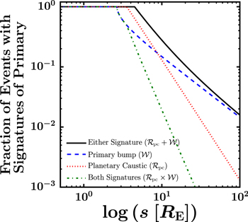
Figure 1. Fraction of planetary microlensing events for which signatures of primary are expected to be detectable , i.e., the fraction of planetary events we can distinguish as being due to bound planets rather than free-floating planets (assuming ML = 0.3 M⊙,  ,
,  , and
, and  ). We examine two channels for detecting signatures of the primary: (1) relatively long-timescale, low-magnification primary bump, and (2) anomalies near the peak of the light curve due to the source passing near (or crossing) the planetary caustic. The relative probabilities of these channels fall off with increasing projected separation as
  and
and  , respectively. See the text for a more detailed description.
Download figure:
Standard image High-resolution image
Figure 2. The lens mass function we adopt in this study (identical to "Model 1" of Sumi et al. 2011), consisting of populations of brown dwarfs, main-sequence stars, white dwarfs, neutron stars, and black holes, each of which is described by a power-law distribution in their initial mass. The top left panel plots the initial lens mass function, and the top right panel plots the final lens mass function. The bottom left and bottom right panels show the final mass function, weighted by lens mass and event rate ( along a given sight line and at fixed Dl, Ds, and
  ), respectively.
Download figure:
Standard image High-resolution imageAlthough it is clear that a majority of the 10 events with tE < 2 days must be due to planetary-mass lenses (if they are indeed due to microlensing and standard models for the distributions of  and μrel are accurate), it is not certain whether these objects are gravitationally bound to a host star or if they are free-floating planets. Sumi et al. (2011) searched for signatures indicative of the presence of a host star in the light curves of the short-timescale events and found nothing (see Section 3 for details on how to distinguish wide-separation planets from unbound planets), but were able to place limits on the projected separation (in units of the Einstein radius), s, of each planet from the host lens under the assumption that one exists (see their Table 1). These limits range between 2.4 ≤ smin ≤ 15.0, which roughly corresponds to semimajor axes between
  assuming a typical primary lens, event parameters, and the median projection angle of a circular orbit, with a median value of smin ≃ 4.2 (amin ≃ 12 au). Here, the variables smin and amin represent the minimum values of the projected separation and corresponding semimajor axis (assuming a randomly oriented, circular orbit), respectively, that would be plausible given the non-detection (at the 2σ level) of features in the microlensing light curves that would indicate the presence of a host star. We note that Sumi et al. (2011) did find three short-timescale events that clearly showed both binary lens caustic crossing features and very low-amplitude signals due to lensing by the primaries (see Bennett et al. 2012 for an analysis of these three events, one of which was the first planetary microlensing event in which the host star was detected only through binary lensing effects, MOA-bin-1), but none of these passed all their selection criteria and made it into their final sample.
Table 1. Median Values and 68% Uncertainties Inferred by Clanton & Gaudi (2016) for the Parameters of a Population of Planets That is Consistent with Results from the Microlensing Surveys of Gould et al. (2010) and Sumi et al. (2010), the Gemini Deep Planet Survey (Lafrenière et al. 2007) and Planets around Low Mass Stars (Bowler et al. 2015) Direct Imaging Surveys, and the CPS TRENDS (Montet et al. 2014) RV Survey
| Planet Evolutionary | Median Values and 68% Uncertainties | |||
|---|---|---|---|---|
| Model | α | β |
![${ \mathcal A }\,[{\mathrm{dex}}^{-2}]$](https://content.cld.iop.org/journals/0004-637X/834/1/46/revision1/apjaa4d0eieqn27.gif)
|
![${a}_{\mathrm{out}}\,[\mathrm{au}]$](https://content.cld.iop.org/journals/0004-637X/834/1/46/revision1/apjaa4d0eieqn28.gif)
|
| "Hot-Start" (Baraffe et al. 2003) |

|

|

|

|
| "Cold-Start" (Fortney et al. 2008) |

|

|

|

|
Download table as: ASCIITypeset image
Since these microlensing data alone are insufficient to constrain the fraction of the population of planetary-mass lenses that are truly unbound, Sumi et al. (2011) consulted results from the Gemini Deep Planet Survey (GDPS; Lafrenière et al. 2007) that place upper limits on the frequency of wide-separation (10 ≲ a/au ≲500) Jupiter- and super-Jupiter-mass planets. Using the information contained in Figure 10 of Lafrenière et al. (2007), Sumi et al. (2011) estimated that <40% of the population of planetary-mass objects required to explain the overabundance of short-timescale microlensing events can be gravitationally bound to a host star at separations between 10–500 au, assuming any such planets have a uniform distribution of  .
.
However, we argue that the use of the full GDPS sample to constrain this fraction of bound planets is not correct (although we show in Section 5 that our final result is actually consistent with the fraction estimated by Sumi et al. 2011). The stellar samples of the Sumi et al. (2011) survey and the GDPS are quite different, and thus the upper limits on planet frequency derived from the full GDPS sample are not necessarily representative of those for only the M stars. This is an important point because microlensing samples are dominated by low-mass lens stars due to the fact that the rate of microlensing events depends explicitly on the mass function of lenses, which is weighted in favor of low-mass stars. On the other hand, the GPDS sample is comprised primarily of FGK stars, with a smaller number of M stars; of the full sample of 85 stars, just 16 are classified as M spectral types. While these stars are generally young, they are old enough that the lower-mass stars probably have spectral types that are not significantly different than what they will have when they fall on the main sequence. By comparing their observed K-band magnitudes to those predicted by stellar isochrones of M stars at similar ages, we argue that most, if not all, of the stars classified as M spectral types in the GDPS sample have a high likelihood of being an analogous population to the low-mass stars that produce the majority of microlensing events toward the Galactic bulge (see Clanton & Gaudi 2016 for discussion). This issue has been pointed out in Quanz et al. (2012), who perform a more careful analysis using the GDPS constraints for just the M stars to estimate the upper limit on the fraction of the population of planetary-mass objects responsible for the observed short-timescale events that are bound to a host star, fmax. These authors found a value of fmax = 0.78 (at 95% confidence) if these planets have a typical mass of 1 MJup and have separations equal to amin that Sumi et al. (2011) calculate for each of the short-timescale events. If the planets are located at separations of 2amin, then fmax = 0.49. Of course, the true planet population (assuming such a bound population exists) will have some distribution of separations, and will directly affect the value of fmax. Another potential issue affecting both the Sumi et al. (2011) and Quanz et al. (2012) analyses is that the GDPS sensitivites (in terms of planet mass) they employ assume "hot-start" planet evolutionary models (Baraffe et al. 2003), which represent the most optimistic predictions for detecting planetary companions via direct imaging.
In this paper, we perform a thorough joint analysis of microlensing, radial velocity, and direct imaging constraints, selecting samples of stars similar to that probed by the Sumi et al. (2011) survey and considering both "hot-" and "cold-start" planet evolutionary models to determine the expected timescale distribution of wide-separation, bound planets whose microlensing light curves reveal no evidence of the host stars they orbit. We will also carry out a more robust analysis than those of either Sumi et al. (2011) or Quanz et al. (2012) by including a distribution of planetary separations, including an outer cutoff semimajor axis for the population, to compute the fraction of the short-timescale events that are due to free-floating planets.
3. DISTINGUISHING BETWEEN MICROLENSING EVENTS DUE TO WIDE-SEPARATION AND FREE-FLOATING PLANETS
In a microlensing event due to a wide-separation ( , where s is the projected separation in units of the Einstein radius) planet, evidence for boundedness can be obtained through three channels: (1) observation of a relatively long-timescale (and likely low-magnification) bump due to the source trajectory passing near enough to the primary to produce a detectable magnification, (2) observation of anomalies near the peak of the light curve due to the source passing near (or crossing) the planetary caustic (Han & Kang 2003), and/or (3) detecting blended light from the primary. The last channel requires data of sufficient angular resolution to resolve out any unrelated stars, so that any additional flux above that of the source is due to the host lens (or a companion to the lens or source). MOA-II data typically have seeing ranging between 1.9–3.5 arcsec, with a median of ∼2.5 arcsec (Bond et al. 2001; Sumi et al. 2003), and thus any detected blend flux could be (and is likely) due to unrelated stars, rather than the lens itself. The presence (or lack) of any blend flux in MOA-II data therefore provides no diagnostic power on the boundedness of planetary lenses. Consequently, Sumi et al. (2011) were only able to look for evidence of a host lens in their 10 short-timescale events through the first two channels and so we do not need to consider the third channel in this study.
Detection of either a primary bump or anomalies due to the planetary caustic depends on the geometry of the event and the quality of the observations (e.g., total number of observations, cadence, photometric precision). For a given set of observational (i.e., survey) parameters, the fractions of events due to wide-separation planets for which the presence of a primary is expected to be detected by these two different channels scales as ∼s−1 and ∼s−2, respectively. In this section, we provide brief descriptions of these two channels and how we implement them in this study, but for a more in-depth look at distinguishing events due to wide-separation and free-floating planets, see Han et al. (2005) and references therein.
3.1. Low-magnification Primary Bumps
The source trajectory in some fraction of planetary microlensing events,  , will be such that the impact parameter to the primary, u⋆, is small enough that it will produce a detectable magnification. For a given observational cadence and signal-to-noise ratio (S/N;
  ) threshold, this fraction depends solely on the geometry of the lens system and has the form
where  is the projected separation of the center of the planetary caustic from the host star and
  is the maximum source impact parameter to the primary in units of the primary Einstein radius,
  , such that the primary bump is just detectable. The form for the maximum impact parameter we adopt is given by Han et al. (2005) as
where ML is the primary lens mass, fobs is the frequency of observations, σp is the fractional photometric precision of each observation, and  is the S/N threshold for detection. The values to which we have scaled this relation are set by the selection criteria of the Sumi et al. (2011) study and are typical for MOA-II data (T. Sumi 2016, private communication). For the given survey parameters (fobs, σp, and
  ) and at fixed primary lens mass (ML), we find that
  out to projected separations s ≲ 2.6. In the limit of large projected separations,
  , the probability of detecting the primary through this channel falls off as s−1. We note that
  is only weakly dependent on fobs, ML, and σp and thus argue that our approximation that these parameters are the same for all events is reasonable. Figure 1 shows a plot of
  and illustrates the that, for parameters typical of the MOA-II survey and the selection criteria set by Sumi et al. (2011), this is not the primary channel for detecting signatures of the host lens except at separations beyond s ≳ 10 (a ≳ 28 au).
3.2. Anomalies Due to the Planetary Caustic
The rate of planetary events where signatures of the primary due to anomalies near the peak of the light curve arising from the source passing near (or crossing) the planetary caustic relative to the total rate of planetary microlensing events is
where  is the maximum required impact parameter for signatures of the planetary caustic to be just detectable as a function of the projected separation, s, and
  is the median impact parameter measured by Sumi et al. (2011) for the 10 short-timescale (
 ) events in their sample. If the MOA-II survey were uniformly sensitive to events with respect to impact parameter, then we would have chosen to normalize
  by u0 = 1, the maximum impact parameter allowed by the criteria set by Sumi et al. (2011), with which they selected their sample (see Section 2 of the supplemental materials of Sumi et al. 2011). In reality, there is a bias toward smaller impact parameters (since the total magnification, A, depends on the lens-source projected separation, u, as
 ![$A(u)=[({u}^{2}+2)/(u\sqrt{{u}^{2}+4})]$](https://content.cld.iop.org/journals/0004-637X/834/1/46/revision1/apjaa4d0eieqn54.gif) ) and we therefore attempt to account for this by normalizing
) and we therefore attempt to account for this by normalizing  by
by  .
.
We assume that in order for signatures of the planetary caustic to be detectable in the light curve that  , where
  is the angular radius of the planetary caustic, which we assume to be circular in shape with a size given by the height of the caustic in the direction perpendicular to the star–planet axis. Adapting Equation (9) of Han (2006) to be consistent with our adopted geometry, we find the following expression for θc (which has units of the primary Einstein radius)
There is a projected separation, sc, at which  and interior to which
  , as defined by Equation (3), becomes greater than unity. This works out to be
  , which roughly corresponds to a projected separation in physical units of
  for typical event parameters and a semimajor axis of ac ≈ 12 au for the median projection angle of a circular orbit. Thus, to ensure that
  , we adopt the definition
and Equation (3) takes the form
In doing so, we are effectively assuming that if a planetary event with  is detected, anomalies due to the planetary caustic will always be detected. For our purposes, this is not a problem, since we are only concerned with computing the fraction of events for which we expect to see evidence of a primary (regardless of the exact channel). Figure 1 illustrates our expectation that for s ≲ 10, perturbations due to the planetary caustic are the primary channel for revealing the presence of a host star.
Note that each of the curves in Figure 1 represents our prediction for the fraction of events where the primary is detected; they are distinguished by the channel through which the primary is discovered (i.e., the type of signal that reveals their existence). Thus, for the events in which the primary is detected, the timescale distribution is simply that of the primaries themselves. Alternatively, in the events for which the primary is not detected, the question as to what the timescale distribution looks like is precisely what we are attempting to determine in this paper (under the assumption that a maximal amount of short-timescale events are due to bound planets which only appear to be free-floating due to mostly geometrical reasons, and partly dependent on the systematics of the MOA-II survey, that are outlined in Section 3). The timescale distribution therefore depends on the distributions of planet masses and semimajor axes.
4. METHODOLOGY
In Clanton & Gaudi (2016), we performed a joint analysis of results from five different surveys for exoplanets employing three independent discovery techniques: microlensing (Gould et al. 2010; Sumi et al. 2010), radial velocity (specifically, the long-term trends; Montet et al. 2014), and direct imaging (Lafrenière et al. 2007; Bowler et al. 2015). We found that the results of all these surveys can be simultaneously explained by a single population of planets described by a with a simple, joint power-law distribution in mass and semimajor axis given by
This model has just four free parameters,  , where aout is the outer cutoff radius of the semimajor axis distribution. The median values and 68% confidence intervals we infer for these parameters are summarized in Table 1. Note that the quoted uncertainties, particularly those on β and aout, are correlated (see Figures 25–27 in Clanton & Gaudi 2016). In this paper, we employ this population of bound planets that is known to be consistent with microlensing, RV (long-term trend detections), and direct imaging surveys to explain (at least a significant fraction) of the overabundance of short-timescale microlensing events observed in the MOA-II data, and thus derive constraints on the frequency of truly free-floating planets in the Galaxy.
We first sample the posterior distributions (including covariances) derived in Clanton & Gaudi (2016) to obtain parameters (i.e., α, β,  , and aout) for a random population of (bound) planets, and draw an ensemble of planets from the resultant distribution function. We then generate a corresponding set of simulated microlensing events, precisely following the procedure we outline in Clanton & Gaudi (2014a, 2014b, 2016), but with a slightly altered LMF. In this paper, we adopt "Model 1" exactly as it is presented in Sumi et al. (2011), which includes populations of brown dwarfs, main-sequence stars, white dwarfs, neutron stars, and black holes that are described by power-law distributions in their initial mass. We fix the slope of the LMF in the brown dwarf regime to be the median value reported by Sumi et al. (2011), as the inferred value for this slope is not significantly different when the fitting the full timescale distribution versus fitting the timescale distribution for
  days (which we verified with our own, completely independent, fitting procedures). Furthermore, analyses of photometric studies (Parravano et al. 2011; McKee et al. 2015) have shown that the mass function is continuous between the low-mass star and brown dwarf regimes and has a slope that is consistent with that determined by Sumi et al. (2011). We display a plot of the initial lens mass distribution (relevant for the remnant populations) in Figure 2, along with plots of the final LMF weighted by number, mass, and contribution to the microlensing event rate along a given line of sight.
The distinction between the initial and final lens mass functions is only relevant for the white dwarf and neutron star populations. The initial lens mass function for these two populations has a power-law form that is normalized with respect to the power-law mass distributions of the other populations (main-sequence stars, brown dwarfs) and is used to determine the numbers of lenses from these remnant populations relative to those of the other populations. The white dwarfs and neutron stars are evolved and have undergone significant amounts of mass loss, thus their final masses have a different distribution from their "initial" masses.
The relative numbers of brown dwarfs, main-sequence stars, white dwarfs, neutron stars, and black holes by number, mass, and event rate are (38:52:9.5:1.1:0.16), (5.9:63:22:5.7:3.2), and (17:63:17:2.9:0.84), respectively (consistent with Gould 2000). We find, as did Sumi et al. (2011), that the numbers of brown dwarfs, white dwarfs, neutron stars, and black holes relative to main-sequence stars are (73:18:2.1:0.31).
We describe in Section 5.1.1 of Clanton & Gaudi (2014a) the details of the Galactic model we choose to adopt in this study (that of Han & Gould 1995a, 1995b, 2003). Although we perform our own normalization of the disk and bulge density functions, we find a consistent microlensing optical depth with Han & Gould (2003). We find that along a line of sight toward Baade's window (l = 1°, b = −3 9), roughly 60% of the lenses are located in the Galactic bulge. This is consistent with the predictions of Kiraga & Paczynski (1994), who considered a completely different Galactic model. Incidentally, we do not know if the lenses that produced the short-timescale events observed by MOA-II are located in the bulge or the disk, as we have no observational constraints on their distances or proper motions relative to the sources. In fact, the short-timescale events individually provide no real constraints on their masses either; it is only when we look at the full sample of observed microlensing events and assume the corresponding lenses have similar kinematic properties as the stellar populations that we notice an excess of short-timescale events that allows for a statistical argument that most of the short-timescale events must be due to planetary-mass objects.
The density model we adopt is used to determine the relative event rates of our ensembles of simulated microlensing events (see Equation (33) of Clanton & Gaudi 2014a). If we were to adopt a different density model, as long as it produced event rates that are not signifcantly different than those of our canonical density model, our results would not be significantly different. While we do not repeat our calculations assuming different sets of Galactic models, we have performed calculations to provide some degree of confidence in our choice (e.g., the optical depths mentioned previously and the fraction of bulge to disk events). Finally, our density model produces a timescale distribution (for  days) that very closely matches the observed distribution presented in Sumi et al. (2011). We provided more discussion about this potential source of uncertainy in Section 5.3.3 of Clanton & Gaudi (2014a) and Section 6.2 of Clanton & Gaudi (2014b).
Figure 3 shows a plot of the predicted distribution of timescales for the brown dwarf, main-sequence, and remnant lenses in our simulated sample against the observed distribution. Our predicted distribution has been corrected for the detection efficiency determined by Sumi et al. (2011) (shown in Figure S2 of their supplemental materials) and normalized such that the total number of simulated microlensing events matches that of the observed sample. Note that this is not a fit to the observed distribution, but rather it is a prediction based on a fit performed by Sumi et al. (2011) that we use to fix the slope of the LMF in the brown dwarf regime. By eye, this appears to be a good match for events with tE > 2 days (providing a degree of confidence in our adopted Galactic model and LMF), but the overabundance of shorter-timescale events in the observed distribution is clear. We will attempt to explain these short-timescale events with bound planetary companions for which we do not expect to see evidence of a primary in the microlensing light curves.
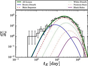
Figure 3. Predicted timescale distribution for populations of brown dwarfs, main-sequence stars, and stellar remnants (colored lines) and the observed timescale distribution reported by Sumi et al. (2011) (black histogram). The predicted timescale distribution has been subjected to the measured detection efficiency of the Sumi et al. (2011) survey and normalized to the total number of observed microlensing events. The number of short-timescale microlensing events (tE ≤ 2 days) predicted by our adopted LMF is 1.1, compared to the observed number of 10, demonstrating a clear overabundance of such short-timescale events in the observed sample.
Download figure:
Standard image High-resolution imageHaving generated a population of planets with corresponding microlensing events as described above, we then determine the probability that the primary (i.e., host star) would not be detected in each event given the survey parameters of MOA-II, ![${P}_{\star }^{\prime }=[1-{ \mathcal W }(s)]\times [1-{{ \mathcal R }}_{\mathrm{pc}}(q,s)]$](https://content.cld.iop.org/journals/0004-637X/834/1/46/revision1/apjaa4d0eieqn69.gif) , where
, where  is the fraction of events where a low-magnification primary bump is expected to be detectable and
  is the fraction of events where perturbations in the light curve due to the planetary caustic are expected (see Section 3 for the formal definitions and a discussion of these quantities). We then construct the predicted timescale distribution for the combination of our adopted LMF and the associated population of bound planets that appear to be free-floating, again taking care to correct for the detection efficiency of MOA-II to events as a function of tE. This predicted timescale distribution serves as our likelihood function (for which there is no analytic form). We calculate the likelihood of a given planet population by applying this numerically generated likelihood function to the individual measurements of tE for each of the 474 events comprising the observed distribution presented in Sumi et al. (2011). These data are published in Table 4 of Sumi et al. (2013). We repeat this procedure for all planet populations Clanton & Gaudi (2016) found to be consistent with radial velocity, microlensing, and direct imaging surveys. This allows us to place constraints on the fraction of short-timescale (
 days) microlensing events due to free-floating planets. In order to determine an actual number of such planets (e.g., relative to main-sequence stars), we must adopt an ad hoc form for the mass function of free-floating planets. Therefore, our estimate of the number of free-floating planets per star is less robust (i.e., more model dependent) than our estimate of the fraction of short-timescale events due to free-floating planets. We present and discuss our results and main sources of uncertainty in the following section.
5. RESULTS AND DISCUSSION
Figure 4 shows the best-fit (i.e., maximum likelihood) expected timescale distribution for the combination of our canonical LMF described in the previous section with populations of wide-separation, bound planets found by Clanton & Gaudi (2016) to be consistent with results from radial velocity, microlensing, and direct imaging surveys for either "hot-start" (Baraffe et al. 2003) or "cold-start" (Fortney et al. 2008) planet evolutionary models. Given that the parameters of these planet populations (i.e., the slopes of the mass function, α and semimajor axis function, β, normalizations,  , and outer cutoff radii, aout) for the "hot-start" and "cold-start" models are not too different (see Section 5.2 of Clanton & Gaudi 2016), it is not surprising that the fits for these different models shown in Figure 4 are so similar. The parameter values for the best-fit "hot-start" planet population are α = −0.85, β = 0.091,
  , and aout = 740 au, and those for the best-fit "cold-start" population are similar. The value of aout for this best fit is quite large due to the fact that the number of planets for which we do not expect to see signatures of a primary lens (host star) in the microlensing light curves (which are needed to explain the overabundance of short-timescale events) increases with this outer cutoff radius. For large aout, planets are allowed to be in very wide-separation orbits which lead to smaller planetary caustic sizes (and thus small rates of planetary caustic events, since at fixed q,
  for s ≫ 1) and which have low probability for source trajectories that pass near the primary (∝s−1 for s ≫ 1). However, in order for a planet population with a large value of aout to be consistent with the non-detections from direct imaging surveys (i.e., Lafrenière et al. 2007 and Bowler et al. 2015), the slope of the semimajor axis distribution function must be shallow, and indeed, the best-fit population has β near zero (corresponding to Öpik's law; Öpik 1924).

Figure 4. Maximum likelihood fits to the observed timescale distribution (black histogram; Sumi et al. 2011) for our canonical LMF and a population of bound, wide-separation planets that is consistent with results from radial velocity, microlensing, and direct imaging surveys (Clanton & Gaudi 2016), assuming either "hot-start" (blue lines; Baraffe et al. 2003) or "cold-start" (red lines; Fortney et al. 2008) planet evolutionary models. The thick lines show the expected timescale distribution from all lenses, while the thin lines show the expected contributions from planets (the curves peaking at shorter timescales) and brown dwarfs, main-sequence stars, and remnants (the curves peaking at longer timescales). For these maximum likelihood fits, wide-separation, bound planets account for roughly 2.9 of the 10 observed short-timescale (tE < 2 days) events in both the "hot-start" and "cold-start" cases, and brown dwarfs account for about one event.
Download figure:
Standard image High-resolution imageIn Figure 5, we display the best-fit to the observed timescale distribution along with the range of fits in the 68% confidence interval. It is clear from this figure that while we can explain some fraction of the short-timescale events with bound, wide-separation planets, an overabundance remains (particularly at timescales between 1–2 days). This suggests that either our assumed planet population model is incorrect in regions of parameter space where we currently have no observational constraints ( at separations a ≳ 10 au), or free-floating planets are responsible for the remaining short-timescale events. We have no way of testing the former, but for the latter case we can constrain the fraction of short-timescale events that would be due to free-floating planets given our assumed planet model.
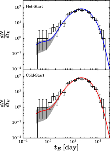
Figure 5. Maximum likelihood and 68% confidence interval fits to the observed timescale distribution (black histograms; Sumi et al. 2011) for our canonical LMF and a population of bound, wide-separation planets that is consistent with results from radial velocity, microlensing, and direct imaging surveys (Clanton & Gaudi 2016), assuming either "hot-start" (top panel; Baraffe et al. 2003) or "cold-start" (bottom panel; Fortney et al. 2008) planet evolutionary models.
Download figure:
Standard image High-resolution imageFor each planet population we fit to the observed timescale distribution, we determine the number of residual events with  and divide by the number of observed events in this same range of tE to compute the fraction of such events which are expected to be due to free-floating planets, fff. We plot the posterior distribution of fff in Figure 6 and report the corresponding median values, 68%, and 95% confidence intervals in Table 2. The posterior for the "cold-start" case is shifted slightly toward lower fff, as expected, but it is not significantly different from the "hot-start" case.

Figure 6. The fraction of short-timescale (tE < 2 days) microlensing events that must be due to free-floating planets, fff, for our analyses that assume either "hot-start" (blue; Baraffe et al. 2003) or "cold-start" (red; Fortney et al. 2008) planet evolutionary models. The vertical, black lines mark the median values of these posterior distributions.
Download figure:
Standard image High-resolution imageTable 2. Median Values, 68%, and 95% Confidence Intervals on Both the Fraction of Short-timescale Events Due to Free-floating Planets, fff, and the Number of Free-floating Planets Relative to Main-sequence Stars, Nff
| Planet Evolutionary | Median | 68% Confidence | 95% Confidence | |
|---|---|---|---|---|
| Model | Value | Interval | Interval | |
| fff | "Hot-Start" | 0.67 | 0.44–0.78 | 0.23–0.85 |
| "Cold-Start" | 0.58 | 0.40–0.74 | 0.14–0.83 | |
| Nff | "Hot-Start" | 1.4 | 0.94–1.7 | 0.48–1.8 |
| "Cold-Start" | 1.2 | 0.86–1.6 | 0.29–1.8 |
Note. We report these values for our analyses that assume either "hot-start" (Baraffe et al. 2003) or "cold-start" (Fortney et al. 2008) planet evolutionary models.
Download table as: ASCIITypeset image
The response of the final normalization of the bound planet timescale distribution with which we attempt to fit the short-timescale event excess to the set of parameters  is quite complex. The relation between this final normalization to
  is the easiest to understand, as it is directly proportional. However, the response to α is governed by the conflation of two separate effects: (1) the event rate is proportional to the square root of the lens mass, meaning that the smaller-mass objects have a lower event rate, and therefore values of α that would favor low-mass (high-mass) planets, would work in the direction of a lower (higher) bound planet timescale distribution normalization, and (2) the overall occurrence rate of planets (i.e., the integral of
  ) depends on α in a non-monotonic fashion (for fixed β,
  , and aout, there is a value of α that minimizes this integral; see Section 3.1.1 of Clanton & Gaudi 2016 for further discussion on this particular issue). Similarly, the response of the final bound planet timescale distribution normalization to the parameter β is governed by the conflation of two distinct effects: (1) as with α, the overall occurrence rate of planets depends non-monotonically on β (for fixed α,
  , and aout, there is a value of β that minimizes the integral, for the same mathematical reasons as with α), and (2) β determines the distribution of the semimajor axes of planets, so for values of β that favor close-separation (wide-separation) planets, the final normalization tends to decrease (increase), since planets that are distributed close to their host stars would have a high probability of being detected as bound exoplanets (and thus not contribute to the timescale distribution we can use to constrain the short-timescale events) and planets that are distributed at wide separations have a smaller probability of being detected as bound exoplanets (by either primary bump or planetary caustic perturbations). Finally, the final bound planet timescale distribution normalization depends directly on the parameter aout (however, not via a simple proportionality, since our model is a joint power-law); at fixed α, β, and
  , larger values of aout increase the overall occurrence rate of exoplanets, and allow for planets to be distributed further from their host stars (where they have relatively lower probabilities of being detected as bound), both of which would lead to a larger final normalization, but (by the same reasoning) smaller values of aout lead to a smaller final normalization.
As part of our fitting procedure, we simultaneously consider the constraints from microlensing, RV, and direct imaging surveys, such that if we were to change any of the parameters  to increase the final normalization of the bound planet timescale distribution (and thus explain a larger fraction of the short-timescale microlensing events as being due to bound, rather than free-floating, planets), we would violate the constraints of one, or several, of the surveys we include. In Figures 5 and 9, we also plot the 68% confidence interval fits, which graphically illustrate the limited flexibility allowed by the survey constraints.
In order to turn the fraction of short-timescale events due to free-floating planets, fff, into an actual number of free-floating planets (relative to main-sequence stars, for example), we must assume a form for their mass function. To this end, we assume that the free-floating planet mass function is given by a Dirac delta function,  . We chose to center the delta function at 2 MJup as such a free-floating planet population leads to a timescale distribution that most closely matches (by eye) the residuals obtained from subtracting off our LMF and the population of wide-separation, bound planets as described in the previous section. Admittedly, this is a rough calculation; however, given the level of precision of this study, we do not believe a more careful analysis is currently warranted (especially given the fact that we currently have no constraints on the actual form of the free-floating planet mass function that we must adopt). The resultant posterior on the number of free-floating planets per main-sequence star is plotted in Figure 7 and the corresponding median values, 68%, and 95% confidence intervals are reported in Table 2. We plot the maximum likelihood fits for the "hot-" and "cold-start" analyses, including the contribution from free-floating planets, under this assumption of a delta-function mass distribution at
  in Figure 8, and we show the range of fits in the 68% confidence interval in Figure 9.

Figure 7. The number of free-floating planets per main-sequence star, Nff, required to explain the residual short-timescale ( days) microlensing events after fits of our canonical LMF and populations of wide-separation, bound planets are subtracted for our analyses that assume either "hot-start" (blue; Baraffe et al. 2003) or "cold-start" (red; Fortney et al. 2008) planet evolutionary models. The vertical, black lines mark the median values of these posterior distributions. Estimating this quantity requires an assumption about the mass function of free-floating planets. Here, we have chosen a delta function at a mass of 2 MJup (see the text for discussion).
Download figure:
Standard image High-resolution image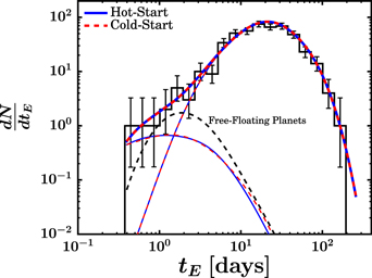
Figure 8. Maximum likelihood fits to the observed timescale distribution (black histogram; Sumi et al. 2011) for our canonical LMF, a population of bound, wide-separation planets that is consistent with results from radial velocity, microlensing, and direct imaging surveys (Clanton & Gaudi 2016), assuming either "hot-start" (blue lines; Baraffe et al. 2003) or "cold-start" (red lines; Fortney et al. 2008) planet evolutionary models, and a population of free-floating planets whose mass function is a δ function at 2 MJup (black dashed line). The thick lines show the expected timescale distribution from all lenses, while the thin lines show the expected contributions from bound planets (the curves peaking at shorter timescales) and brown dwarfs, main-sequence stars, and remnants (the curves peaking at longer timescales). For these maximum likelihood fits, wide-separation, bound planets account for roughly 2.9 of the 10 observed short-timescale ( days) events in both the "hot-start" and "cold-start" cases, brown dwarfs account for about one event, and free-floating planets make up the difference.
Download figure:
Standard image High-resolution image
Figure 9. Maximum likelihood and 68% confidence interval fits to the observed timescale distribution (black histograms; Sumi et al. 2011) for our canonical LMF, a population of bound, wide-separation planets that is consistent with results from radial velocity, microlensing, and direct imaging surveys (Clanton & Gaudi 2016), assuming either "hot-start" (top panel; Baraffe et al. 2003) or "cold-start" (bottom panel; Fortney et al. 2008) planet evolutionary models, and a population of free-floating planets whose mass function is a δ function at  .
.
Download figure:
Standard image High-resolution image
The median number of free-floating planets per main-sequence star we find,  (
( ) for the "hot-start" ("cold-start") case, is quite a large number that seems difficult to explain with any known formation mechanism (see Section 1 for a discussion on the formation channels for free-floating planets). However, more "comfortable" values of Nff = 0.48 (Nff = 0.29; "cold-start") are allowed to within 95% confidence and could perhaps be easier to explain. Furthermore, these values are sensitive to a number of assumptions, most notably the free-floating planet mass function and the model for the population of wide-separation, bound planets. The remainder of this section is devoted to discussion of these two primary sources of uncertainty.
Free-Floating Planet Mass Function. Without direct lens mass measurements for each of the short-timescale events, the only constraining power currently available on the free-floating planet mass function is, in fact, contained in the observed microlensing event timescale distribution. In order to constrain the free-floating planet mass function using the timescale distribution, prior knowledge of which of the short-timescale events are actually due to free-floating planets would be required. With such knowledge, one could perform a model comparison of fits to the observed timescale distribution assuming different forms for the free-floating planet mass function. Unfortunately, we do not know exactly which events are caused by truly unbound planets (due to fundamental degeneracies that affect a majority of microlensing observations; see Gaudi 2012 and references therein) and the number of short-timescale (tE ≲ 2 days) events is small, making such a study difficult. This paper is an attempt to address the first of these issues by simulating microlensing events of wide-separation, bound planets to determine (statistically) the fraction of the short-timescale events that are caused by free-floating planets. Of course, the results presented herein are therefore dependent on our assumed model of bound planets.
In this paper, we assume a simple delta-function form for the free-floating planet mass distribution. Furthermore, we choose the mass at which to center the delta function to be the value which, by eye, most closely matches the residuals of the observed timescale distribution after subtraction of contributions due to our adopted LMF and bound planet populations. In principle, we could perform a formal maximum likelihood analysis on these residuals to more accurately determine the mass and normalization of our free-floating planet delta-function mass distribution. However, the resulting constraints would likely not be very informative, given the fact that we are starting with a sample of just 10 short-timescale events from which we must first subtract contributions due to bound planets, stars, and brown dwarfs (which together account for ∼40%–50% or more, in some cases, of the short-timescale events) to obtain the residuals that would then provide the constraining power. We would therefore only have a few events with which we would be trying to constrain the mass and normalization of the free-floating planet mass function. Thus, given the current data set, we do not believe such an analysis is warranted. The prospect of trying different models for the free-floating planet mass function to explain the residual short-timescale events is even more precarious. A power-law mass function, for example, would require three free parameters: a normalization, an exponent, and a lower-mass cutoff.
Current limitations notwithstanding, data from ongoing and future microlensing surveys will allow direct measurements of both the frequency and mass function of free-floating planets, as well as their spatial distribution within our Galaxy. The recent K2 Campaign 9 (K2C9) consisted of a survey toward the Galactic bulge (Henderson et al. 2015). For short-timescale microlensing events observed simultaneously from Kepler and ground-based observatories (such that we see two distinct source trajectories), it is possible (for some events) to directly measure the lens mass and distance and obtain better constraints on the existence of a primary (i.e., host star) since Kepler provides precise, continuous observations (see Henderson et al. 2015; Henderson & Shvartzvald 2016). However, given the short, ∼80 day duration of K2C9, the sample size will likely be too small to make population-level inferences about free-floating planets other than (at least limits) on their occurrence rates (recall that the event rate scales as  ). Indeed, Penny et al. (2016) predict that K2C9 will detect between 1.4 and 7.9 microlensing events due to free-floating planets (assuming 1.9 free-floating planets per main-sequence star per the Sumi et al. 2011 result). Of these expected detections, Penny et al. (2016) predict that for between 0.42 and 0.98 it will be possible to gain a complete solution (i.e., to measure both finite-source effects and microlens parallax). Given the results we present in this paper, these numbers would be smaller by a factor of ∼0.6 (refer to Table 2), and thus it is unlikely K2C9 will actually directly measure the lens mass in a short-timescale event.
Fortunately, the microlensing survey of the Wide-Field InfraRed Survey Telescope (hereafter WFIRST; Spergel et al. 2015) will ultimately, when combined with ground-based observations, provide the necessary data to directly measure frequencies, masses, and distances for a large sample of free-floating planets with masses down to that of Mars (see Gould et al. 2003 and Yee 2013, who demonstrate that simultaneous observations from the ground and WFIRST at L2 will enable the measurement of the parallax of planetary events, and see Zhu & Gould 2016 for a quantitative analysis of the benefits of a simultaneous ground-based survey to complement the microlensing survey of WFIRST). Depending on the exact occurrence rates, WFIRST will detect ∼hundreds to ∼thousands of free-floating planets (see Tables 2–6 of Spergel et al. 2015).
The Population of Wide-separation, Bound Planets. The model we assume in this paper is a joint power-law distribution function in planet mass and semimajor axis that Clanton & Gaudi (2016) demonstrate to be consistent with results from radial velocity, microlensing, and direct imaging surveys (the caveats and uncertainties of which are laid bare in Section 6 of Clanton & Gaudi 2016). However, the region of planet parameter space we examine in this paper ( a ≳ 10 au) is not directly constrained by any observations. We have implicitly assumed that our distribution function extrapolates into this region of parameter space. It could be the case that the form of the planet mass function depends on semimajor axes for a ≳ 10 au, which could significantly alter our conclusions. For example, if no planets with masses
  form beyond ∼10 au but there is an abundance of slightly less massive planets, we could easily explain most, if not all, the short-timescale microlensing events with bound planets and still satisfy results from all radial velocity, microlensing, and direct imaging surveys of M stars.
Future observations will provide the necessary sensitivity to test the planetary mass function at wide-separations and determine whether or not the mass function measured by microlensing surveys extends further out (as we have assumed to be the case in this paper). The James Webb Space Telescope (JWST; Gardner et al. 2006) is expected to have the capability to achieve contrasts of ∼10−5 at angular separations ≳0.6 arcseconds for observations at ∼4.5 μm with NIRCam (and even greater sensitivity at larger separations; Horner & Rieke 2004; Krist et al. 2007). A survey of nearby, young M stars with JWST/NIRCam as proposed by Schlieder et al. (2016) has the potential to probe down to masses of ∼0.1 MJup at separations of ∼10 au, complementary (and perhaps with some overlap) to microlensing surveys.
6. SUMMARY
In this paper, we attempt to explain the observed overabundance of short-timescale (tE < 2 days) microlensing events with populations of wide-separation, bound exoplanets that are known to be simultaneously consistent with results from radial velocity, microlensing, and direct imaging surveys. We select planetary systems from such populations that we (statistically) expect not to show evidence of a primary (i.e., host star) in their microlensing light curves, either via low-magnification bumps or anomalies near the peak of the light curve due to close approaches to, or crossings of, the planetary caustics. We fit the observed timescale distribution reported by Sumi et al. (2011) with these planetary systems and a primary lens mass function consisting of brown dwarfs, main-sequence stars, white dwarfs, neutron stars, and black holes. We find that wide-separation, bound planets can explain some of the short-timescale events, but (assuming our joint power-law planet distribution function in mass and semimajor axis presented in Clanton & Gaudi 2016 is correct) free-floating planets must account for a fraction of the short-timescale events of either  (0.23–0.85 at 95% confidence) for "hot-start" planet evolutionary models (Baraffe et al. 2003) or fff = 0.58 (0.14–0.83 at 95% confidence) for "cold-start" models (Fortney et al. 2008).
The fraction of short-timescale events due to free-floating planets is the most robust statistic we can infer from the available data (see Section 5). In order to determine an occurrence rate of free-floating planets, we must necessarily assume something about their mass function (for which there are currently no observational constraints). We choose to adopt a free-floating planet mass function that is a delta function at  , as this (roughly) reproduces the residual timescale distribution after subtraction of our canonical LMF and wide-separation, bound planets that are not expected to show evidence of a primary. Under this assumption, we compute the number of free-floating planets per main-sequence star and find a median value Nff = 1.4 (0.48–1.8 at 95% confidence) in the "hot-start" case and Nff = 1.2 (0.29–1.8 at 95% confidence) for the "cold-start" case.
These values are slightly lower than that suggested by Sumi et al. (2011) of  , but still seem difficult to explain given our current understanding of formation channels for free-floating planets. Our results also suggest occurrence rates of free-floating planets that are higher by a large factor than those inferred by the SONYC imaging survey of NGC 1333 (Scholz et al. 2012b), but quite a bit lower than those inferred by the photometric survey of the ρ Oph cloud core by Marsh et al. (2010). Potential reasons for the differences in frequencies of free-floating planets between our results and those of imaging surveys are (1) imaging surveys are probing a different population of free-floating, planetary-mass objects, (2) these frequencies are heavily dependent on the local environmental conditions, (3) the imaging surveys, which are only typically sensitive to objects more massive than about a couple of Jupiter masses, lack the sensitivity to probe the free-floating planet population inferred by microlensing.
Future observations will be critical to further elucidate the true abundance and demographics of free-floating planets. Direct mass measurements of a statistically significant sample of short-timescale microlensing events will allow us to infer the mass function of free-floating planets. It is unlikely that there will be any lens mass measurements from short-timescale microlensing events from the K2 Campaign 9 data set (see Section 5), but as Penny et al. (2016) point out, K2C9 can still test the hypothesis that these events are, in fact, due to planetary-mass objects and, if so, whether or not they are bound to stars. Ultimately, the microlensing survey of WFIRST will provide robust measurements of the free-floating planet mass function, their occurrence rates, and their Galactic distribution (Spergel et al. 2015).
We thank Takahiro Sumi and Radek Poleski for helpful conversations. This research has made use of NASA's Astrophysics Data System and was partially supported by NSF CAREER Grant AST-1056524. Work by C.D.C. was supported by an appointment to the NASA Postdoctoral Program at the NASA Ames Research Center, administered by Universities Space Research Association under contract with NASA.
Footnotes
- 4