


Abstract
Aerosols in the atmospheres of cloudy gas giant exoplanets and brown dwarfs scatter and polarize these objects' thermal emission. If such an object has an oblate shape or nonuniform cloud distribution, the net degree of linear polarization can show an increase ranging from several tenths of a percent to a few percent. Modern high-contrast imaging polarimeters are now poised to detect such low-polarization signals, opening up a new window into the rotational velocities and cloud properties of substellar companions to nearby stars. In this paper, we present the results of a near-IR survey searching for linearly polarized thermal emission from a sample of two planetary-mass companions and five brown dwarf companions using GPI and SPHERE-IRDIS. We probe the subpercent linear polarization regime that typifies polarized free-floating brown dwarfs and place limits on each object's degree of linear polarization. We relate our upper limits on each target's degree of linear polarization to its rotation rate, and place our results in the context of rotation rates measured using high-resolution spectroscopy.
Export citation and abstract BibTeX RIS
1. Introduction
Observations of gas giant exoplanets and brown dwarfs indicate that clouds and hazes are ubiquitous in the atmospheres of substellar objects (e.g., Allard et al. 2001; Burgasser et al. 2002; Marley et al. 2002; Tsuji 2002; Marois et al. 2008; Barman et al. 2011). So far, this feature has largely hampered atmospheric characterization efforts: the red colors of young substellar objects are best explained by models that include thick photospheric clouds, but the radii predicted by these models are inconsistent with evolutionary models (e.g., Bowler et al. 2010; Liu et al. 2013; Tremblin et al. 2017). Such discrepancies may be due to poorly constrained cloud grain size distributions, depth variations, and horizontal structures.
However, clouds and hazes also offer observational opportunities: aerosols in the atmospheres of young, cloudy substellar objects scatter and polarize these objects' thermal emission (Sengupta & Krishan 2001). While a perfectly spherical, uniformly cloudy object has zero net polarization, an oblate shape or nonuniform cloud patterns (like Jupiter's belts and zones) can bring the net degree of linear polarization to ≤2% (de Kok et al. 2011; Marley & Sengupta 2011; Stolker et al. 2017). Since Ménard et al. (2002) reported the first detection of linearly polarized brown dwarf radiation, several studies have sought to link polarimetric observations of substellar objects with their physical interpretations. For example, Miles-Páez et al. (2013, 2017a) find a correlation between the detection of polarized brown dwarf emission and rotation, where the rotation is based on  and photometric variability measurements, respectively. These results are suggestive of oblateness-enhanced polarization. The observational case for polarization from surface inhomogeneities, however, is less developed. Observations of the photometric variability of the planetary-mass companion 2M1207 b, as well as of brown dwarfs of similar temperatures, indicate that young substellar companions' clouds are frequently patchy (Crossfield et al. 2014; Radigan 2014; Zhou et al. 2016). It has been shown by de Kok et al. (2011) that such patchy atmospheres can lead to time-varying polarimetric signals with amplitudes greater than 0.1%. Indeed, Miles-Páez et al. (2015) found observational evidence that the polarimetric variability of the cool dwarf TVLM 51346546 correlates with rotation. At the same time, detections of photometric variability and polarized emission have not been shown to be statistically correlated (e.g., Sengupta & Marley 2010; Miles-Páez et al. 2017b). Recently, Millar-Blanchaer et al. (2020) detected linearly polarized thermal emission from the L/T transition binary brown dwarf system Luhman 16. While the polarization of Luhman 16 B could be explained either by an oblate, uniformly cloudy atmosphere or by nonuniform cloud coverage, the polarization of Luhman 16 A could only be explained by an inhomogeneous (e.g., banded) cloud structure that is constant over a single rotation period.
High-resolution spectroscopy has recently opened a new window into the rotation rates of planetary-mass companions (Snellen et al. 2014; Bryan et al. 2018; Xuan et al. 2020). Bryan et al. (2018) suggested that planets' spins are set during the late stages of accretion; subsequent theoretical work by Batygin (2018) and Ginzburg & Chiang (2020) found that these results are consistent with planetary spin regulation via magnetic torques between the planet and its circumplanetary disk. Rapidly maturing instrumentation for the high-resolution spectroscopy of faint, close-in companions (e.g., high-dispersion coronagraphy; Snellen et al. 2015; Mawet et al. 2017) will further complete this picture.
Polarimetry constrains the rotation rates of cloudy substellar objects in a way that is independent of and complementary to high-resolution spectroscopy and photometric monitoring (Sengupta & Marley 2010). For example, while both broadband polarimetry and some approaches to high-resolution spectroscopy rely on atmospheric models to connect their observables to rotation rates, the point of connection is different. A high-resolution spectrum is cross-correlated with a model atmosphere broadened to the instrumental resolution, and the resulting cross-correlation function (CCF) is compared with model CCFs representative of a model atmosphere broadened to a given  as well as the instrumental resolution (this model is also offset by a radial velocity). Alternatively, the high-resolution spectrum can be cross-correlated with spectra of slowly rotating brown dwarfs with similar spectral types to the target (Reid et al. 2002; Zapatero Osorio et al. 2006). In contrast, a measurement of an object's degree of linear polarization is related to
  by way of a model spectrum with a particular oblateness and set of dust scattering parameters (Sengupta & Marley 2009, 2010). Furthermore, unlike photometric or spectroscopic monitoring, a single polarimetric observation can flag a target as potentially fast-rotating if it is found to be polarized.
We also note that large discrepancies between these methods may hint at additional physical processes at play: for example, if high-resolution spectroscopic or photometric observations indicate that an exoplanet is rotating so slowly that its oblateness-induced polarization would be undetectable, but the object is nevertheless polarized, we would conclude that the polarized emission is the result of patchy clouds or a circumplanetary disk (de Kok et al. 2011; Stolker et al. 2017).
In Jensen-Clem et al. (2016), we showed that the Gemini Planet Imager (GPI; Macintosh et al. 2014) is sensitive to linear polarization fractions under 2%, using the brown dwarf companion HD 19467 B as a test case. Similarly, van Holstein et al. (2017) demonstrated that the Spectro-Polarimetric High-contrast Exoplanet REsearch instrument (SPHERE; Beuzit et al. 2019) InfraRed Dual-band Imager and Spectrograph (IRDIS; Dohlen et al. 2008) can achieve subpercent polarimetric sensitivity for substellar companions to nearby stars (these results were close to the photon noise limit). The absolute polarimetric accuracy of both instruments is estimated to be ≲0.1% (Wiktorowicz et al. 2014; van Holstein et al. 2020). These capabilities led to the first direct detection of a polarized companion: CS Cha b, a ∼20 MJup substellar companion whose large J-band degree of linear polarization (13.7% ± 0.4%) is best explained by a disk and dust envelope (Ginski et al. 2018).
In this paper, we present the results of a polarimetric survey of two planetary-mass companions and five brown dwarf companions to nearby stars using GPI and SPHERE. Our survey is complemented by the SPHERE-IRDIS polarimetric observations of twenty substellar companions presented in R. G. T. van Holstein et al. (2020, in preparation). The structure of this paper is as follows: in Section 2, we describe our target selection process; in Section 3, we describe the observations and preliminary processing used to generate Stokes cubes from each data set; in Section 4, we retrieve the total intensity and positions of each companion; in Section 5, we measure the polarization of the parent stars; in Section 6, we determine whether polarized thermal emission has been detected and place limits on each object's linear polarization; in Section 7, we relate each object's detection limits to a model of the linear polarization fraction as a function of rotational velocity; finally, our conclusions are given in Section 8.
2. Target Selection
We selected our targets to cover the largest possible range of spectral types, ages, and masses of substellar companions to nearby stars whose flux would allow us to probe polarizations at the 1% level. These targets are listed in Table 1. We note that observations of brown dwarf companions offer several unique advantages compared with polarimetric observations of free-floating brown dwarfs: (1) properties such as the age and metallicity of the brown dwarf can be inferred from the bright primary star; (2) in some cases, radial velocity (RV) and/or astrometric data can be combined with orbital monitoring via imaging, to yield dynamical mass measurements of the companion; (3) the formation pathways of low-mass brown dwarf companions and massive exoplanets are potentially similar, and hence the atmospheres of brown dwarf companions are of particular interest for exoplanet science. Motivated by these advantages, we selected the age/metallicity/mass benchmark companions HR 7672 B (Liu et al. 2002; Crepp et al. 2012), HD 4747 B (Crepp et al. 2016) and HD 19467 B (Crepp et al. 2014). We further selected HR 3549 B (Mawet et al. 2015), a young brown dwarf whose spectrum has been well-characterized with SPHERE/IRDIS (Mesa et al. 2016), as well as HR 2562 B, an intermediate-age brown dwarf with hints of variability that might point toward nonuniform cloud coverage (Konopacky et al. 2016; Mesa et al. 2018). Finally, we selected two planetary-mass companions, β Pictoris b (Lagrange et al. 2010) and ROXs 42 Bb (Kraus et al. 2014), whose rotational velocities have been measured using high-resolution spectroscopy (see Section 7; Snellen et al. 2014; Bryan et al. 2018).
Table 1. Target List
| Target | SpT | Age | Mass (MJup) | Distancea (pc) |
|---|---|---|---|---|
| ROXs 42 Bb | M8−L0b | 1–5 Myrb | 10 ± 4 (atmospheric/evolution models)b |

|
| HR 3549 B | M9−L0c | 100–150 Myrc | 40–50 (atmospheric/evolution models)c |

|
| β Pic b | L2 ± 1d | 24 ± 3 Myre | 13 ± 3 (astrometricf) |

|
| HR 7672 B | L4.5 ± 1.5g | 2.5 ± 1.8 Gyrh |
 (dynamicalh) (dynamicalh) |

|
| HD 4747 B | T1 ± 2i |
 Gyrj Gyrj
|
 (dynamicali) (dynamicali) |

|
| HR 2562 B | T2−T3k |
 Myrk Myrk
|
32 ± 14 (atmospheric/evolution models)k |

|
| HD 19467 B | T5−T7l |
 Gyrj Gyrj
|
 (dynamicall) (dynamicall) |

|
Notes.
aBailer-Jones et al. (2018). bKraus et al. (2014). cMesa et al. (2016). dChilcote et al. (2017). eBell et al. (2015). fDupuy et al. (2019). gLiu et al. (2002). hCrepp et al. (2012). iCrepp et al. (2018). jWood et al. (2019). kMesa et al. (2018). lCrepp et al. (2014).Download table as: ASCIITypeset image
3. Observations and Data Reduction
GPI, SPHERE, and most recently SCExAO/CHARIS are the only instruments currently online that offer the combination of extreme adaptive optics and polarimetric capabilities needed to detect linearly polarized thermal emission from substellar companions to nearby stars. Observations of the targets listed in Section 2 were divided between GPI and SPHERE based on these instruments' fields of view (2 7 × 27 and 11'' × 11'', respectively) and limiting host star magnitudes for optimal adaptive optics performance (I < 9 and R < 11, respectively). The observations are summarized in Table 2. The GPI and SPHERE polarimetry modes relevant to this study are described below.
Table 2. Summary of Observations
| Target | Date | Instrument | Observing | Exp. Time | Parallactic | Airmass | Seeing ('') | Measured | Measured |
|---|---|---|---|---|---|---|---|---|---|
| Mode | (minutes) | Rotation (°) | Stellar Q/I | Stellar U/I | |||||
| β Pictoris | 2015-12-24 | GPI | J-pol | 61.97 | 38.89 | 1.07–1.10 | 1.02 | −0.64 ± 0.03%a | 0.03 ± 0.01%a |
| β Pictoris | 2015-12-25 | GPI | J-pol | 210.75 | 110.31 | 1.07–1.18 | 0.74 | −0.24 ± 0.02%a | 0.03 ± 0.01%a |
| ROXs 42 B | 2017-03-14 | SPHERE | DPI-J | 139.2 | 8.77 | 1.00–1.27 | 0.41 | 1.69 ± 0.38% | 0.99 ± 0.37% |
| ROXs 42 B | 2017-03-15 | SPHERE | DPI-J | 147.73 | 8.92 | 1.00–1.38 | 0.47 | 1.74 ± 0.3% | 0.94 ± 0.27% |
| HD 4747 | 2017-09-18 | GPI | H-pol | 38.83 | 49.1 | 1.01–1.02 | N/A | 0.01 ± 0.05% | 0.02 ± 0.02% |
| HD 4747 | 2018-08-11 | GPI | H-pol | 53.9 | 25.17 | 1.01–1.07 | N/A | 0.04 ± 0.04% | 0.08 ± 0.04% |
| HD 4747 | 2018-08-15 | GPI | H-pol | 45.63 | 69.78 | 1.01–1.02 | N/A | −0.1 ± 0.03% | 0.06 ± 0.02% |
| HD 19467 | 2017-11-26 | GPI | H-pol | 117.9 | 93.96 | 1.04–1.52 | N/A | −0.02 ± 0.01% | 0.01 ± 0.01% |
| HD 19467 | 2017-11-27 | GPI | H-pol | 31.88 | 21.36 | 1.04–1.06 | N/A | −0.03 ± 0.06% | 0.06 ± 0.01% |
| HR 7672 | 2018-05-20 | GPI | H-pol | 39.79 | 12.27 | 1.48–1.54 | N/A | −0.05 ± 0.03% | 0.01 ± 0.02% |
| HR 7672 | 2018-08-12 | GPI | H-pol | 42.36 | 12.78 | 1.48–1.55 | N/A | −0.1 ± 0.02% | 0.004 ± 0.004% |
| HR 2562 | 2019-02-21 | SPHERE | DPI-H | 33.33 | 19.37 | 1.23–1.25 | 0.93 | 0.08 ± 0.06% | −0.03 ± 0.06% |
| HR 2562 | 2019-02-25 | SPHERE | DPI-H | 48.27 | 24.08 | 1.26–1.37 | 0.91 | 0.07 ± 0.05% | 0.06 ± 0.05% |
| HR 2562 | 2019-03-12 | SPHERE | DPI-H | 48.27 | 27.39 | 1.23–1.26 | 1.0 | 0.08 ± 0.04% | −0.01 ± 0.05% |
| HR 2562 | 2019-03-20 | SPHERE | DPI-H | 48.27 | 24.28 | 1.26–1.35 | 0.97 | 0.07 ± 0.04% | 0.05 ± 0.04% |
| HR 3549 | 2019-03-12 | SPHERE | DPI-H | 35.1 | 18.16 | 1.19–1.24 | 0.84 | 0.09 ± 0.03% | 0.05 ± 0.05% |
| HR 3549 | 2019-03-16 | SPHERE | DPI-H | 35.1 | 18.17 | 1.19–1.24 | 0.92 | 0.1 ± 0.05% | 0.06 ± 0.04% |
| HR 3549 | 2019-03-23 | SPHERE | DPI-H | 35.1 | 19.63 | 1.18–1.20 | 0.96 | 0.02 ± 0.07% | −0.04 ± 0.05% |
Note.
aThis measurement includes the instrumental polarization as well as the stellar polarization. See Section 5 for details.Download table as: ASCIITypeset image
Early in our survey, we chose to observe in the J band, as Marley & Sengupta (2011) predict that the polarization of cloudy, oblate substellar objects will be somewhat higher in the J band than in the H band or K band. Later in our survey, however, it became clear that GPI's systematics were more thoroughly characterized in the H band due to the large number of H-band polarimetric observations made as part of the GPI Exoplanet Survey (Millar-Blanchaer et al. 2017); furthermore, both GPI and SPHERE achieve higher Strehl ratios in the H band. Hence, we later elected to observe in the H band, despite the reduction in the expected polarization signal by up to a few tenths of a percent, depending on the effective temperature and surface gravity (see Marley & Sengupta 2011 Figures 5–7).
3.1. GPI
In GPI's polarimetry mode, the integral field spectrograph's dispersing prism is replaced by a Wollaston prism, and an achromatic half-wave plate (HWP) is inserted between the coronagraph's focal plane and Lyot mask. A polarimetric observing sequence consists of sets of four exposures as the wave plate is rotated through the angles 0 0, 225, 450, and 675. GPI operates in angular differential imaging (ADI) mode, allowing the sky to rotate with respect to the telescope pupil. The Stokes data cube describing the astronomical polarization is computed by inverting the Mueller matrix whose elements represent the polarization induced by the instrument and sky rotation. A detailed description of GPI's polarimetry mode and Stokes cube extraction can be found in Wiktorowicz et al. (2014) and Perrin et al. (2015).
In this study, the Stokes data cubes were constructed from the raw data using the publicly available GPI pipeline v1.4.0 (Maire et al. 2010; Perrin et al. 2014). Our analysis deviates from the public pipeline's default recipes in our treatment of the stellar and instrumental polarization. While the public pipeline, by default, measures and subtracts the combined instrumental and stellar polarization from each individual frame, we subtract only the instrumental polarization values for each HWP position measured from the GPIES campaign data set (Millar-Blanchaer et al. 2017). Hence, we assume that the instrumental polarization in our data follows that of the average GPIES campaign observation—a reasonable assumption, given the proximity and brightness of the parent stars in our sample. This approach allows us to measure the stellar polarization separately from the instrumental polarization (Section 6). The approach described above, however, cannot be applied to our J-band β Pic b data set, as the GPIES campaign data includes only H-band observations. Hence, we must estimate and subtract the combined instrumental polarization and stellar polarization for this target using the GPI pipeline.
We note that, while the crosstalk from Stokes I to Stokes Q and U has been characterized by Wiktorowicz et al. (2012), we do not include crosstalk in our analysis, as we do not expect that it will significantly impact the upper limits presented in Section 6.
To convert the Stokes cube data units from ADU per coadd to electrons, the cube is multiplied by the detector's gain of 3.04e-/ADU and the number of coadds per observation. Representative Stokes I, Q, and U images are shown in Figure 1.
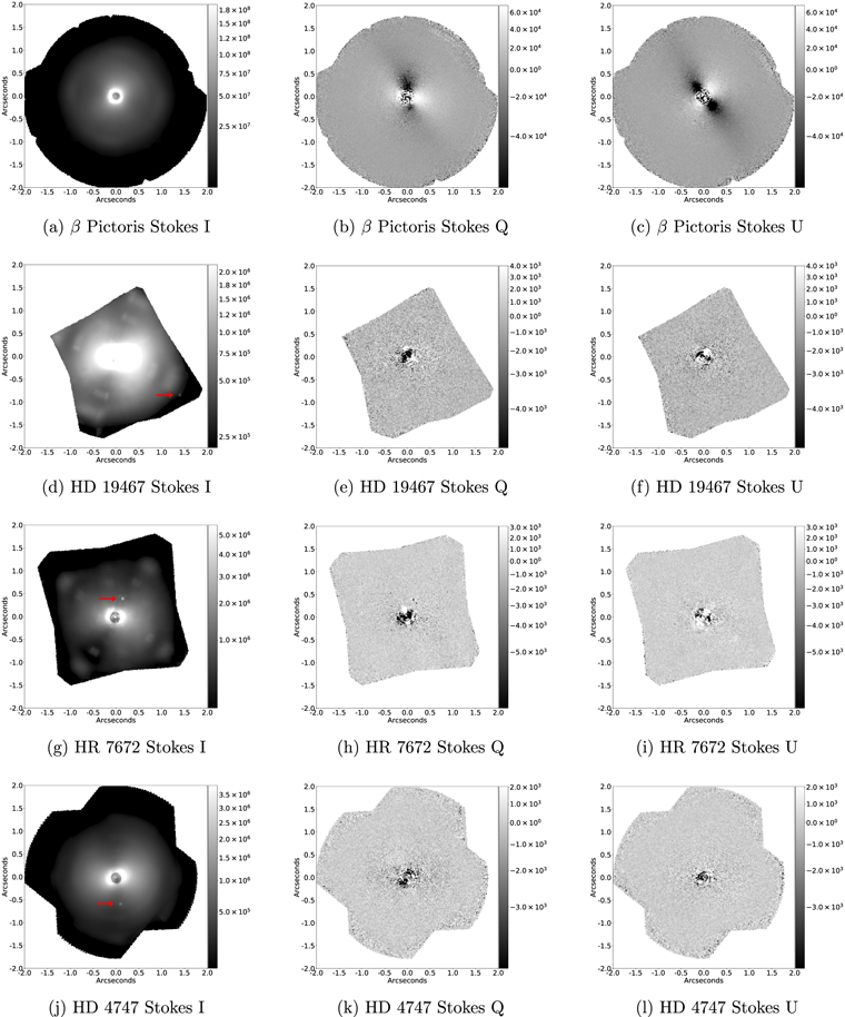
Figure 1. Stokes cubes extracted from observations of β Pictoris (combined 2015 December 24 and 25), HD 19467 (combined 2017 November 26 and 27), HR 7672 (2018 May 20), and HD 4747 (2017 September 18). Red arrows indicate the locations of the substellar companions in the Stokes I frames (β Pic b is not visible in the raw Stokes I frame, but the star's debris disk is evident from the pattern in Stokes Q and U).
Download figure:
Standard image High-resolution image3.2. SPHERE
We observed one planetary-mass companion and two brown dwarf companions to nearby stars (Table 2) with the SPHERE-IRDIS dual-beam polarimetric mode (de Boer et al. 2020; van Holstein et al. 2020). While GPI separates a single beam into orthogonally polarized spot pairs, SPHERE/IRDIS splits the beam in two and uses polarizers with orthogonal transmission axes to create two orthogonally polarized images on the detector. An HWP is then rotated through a sequence of four positions in order to allow the Stokes parameters to be computed via double differencing. We construct Stokes cubes from our raw data using the publicly available IRDIS Data reduction for Accurate Polarimetry pipeline (IRDAP;16 van Holstein et al. 2020). This pipeline includes a Mueller matrix model that mitigates the effects of instrumental polarization and crosstalk, yielding a total polarimetric accuracy of p ≲ 0.1%, where p is the degree of linear polarization (see Section 6). Representative Stokes I, Q, and U images are shown in Figure 2.

Figure 2. Stokes cubes extracted from observations of ROXs 42 B (2017 March 15), HR 2562 (combined 2019 February 21, 25, 2019 March 12, and 20), and HR 3549 (combined 2019 March 12, 16, and 23). Red arrows indicate the locations of the substellar companions in the Stokes I frames. We note that ROXs 42 Bb is clearly detected in Stokes Q and U.
Download figure:
Standard image High-resolution image4. Retrieval of the Total Intensity and Positions of the Companions
In order to measure the separation, position angle, and flux of each companion in our sample, we inject negative template PSFs into the data cubes listed in Table 2 (combining those data sets of a given target that were acquired within one month of each other). We use Markov Chain Monte Carlo (MCMC) to sample the posterior distributions of the template PSFs' separations, position angles, fluxes, and PSF shape parameters (discussed below). Through the Vortex Image Processing (VIP; Gomez Gonzalez et al. 2017) package interface, we use the emcee package (Foreman-Mackey et al. 2013) affine-invariant ensemble sampler for MCMC (Gelman & Rubin 1992).
For GPI targets, the initial template PSF is generated with the AO simulation code presented in Poyneer & Macintosh (2006). The reason for adopting this template PSF rather than making use of GPI's satellite spots (as is done in GPI's spectroscopy mode) is that the satellite spots are elongated in GPI's polarimetry mode due to the full-filter bandpass. For the SPHERE targets HR 3549 B and HR 2562 B, our template PSFs are the average of the short-exposure, unocculted flux frames, obtained twice per observation sequence with a neutral density filter inserted to avoid saturation. Our final SPHERE target, ROXs 42 Bb, orbits a binary star that is barely resolved in our flux frame. To find a suitable PSF to inject into this data set, we identified 53 flux frames from the ESO archive that matched our observational setup, and chose the flux frame whose negative injection gave the best preliminary fit to the companion via VIP's Nelder–Mead-based optimization code.
We are initially interested in measuring the position and flux of the companions in Stokes I only. Hence, for each individual exposure, we sum the two images representing the flux in the two orthogonal directions of polarization, to create a single total-intensity image. We then inject the negative template PSF into the resulting total-intensity data cube. We next choose a method for mitigating residual starlight for each data set. The planet β Pic b is faint compared to the speckles, so we use the VIP implementation of principal component analysis (PCA) to subtract the speckles in a 4× full width at half maximum (FWHM) wide annulus centered on the planet's separation. The remaining companions, however, are bright compared to the speckles at the same separation. We find that ADI/PCA tends to distort the shape of these bright objects' PSFs, and that we generally obtain better residuals by high-pass filtering and median combining the intensity frames after injecting the negative template PSF (we employ a high-pass median filter with a box size equal to the FWHM; see Section 6). We further find that the best-fit residuals for all objects improve if we allow for asymmetry in the template PSF, e.g., allowing the template PSF to stretch in the x and y directions (accomplished by adapting the pyKLIP routine for rescaling images based on varying wavelength), and by allowing the PSF to subsequently rotate. We incorporate these additional PSF characteristics unless their posterior distributions reproduce the flat prior. The posterior distributions for flux, position, and PSF shape parameters in addition to the best-fit residuals are shown in Figures 17–24. Our best estimate of each object's flux and position is taken to be the median of the posterior distribution, with an initial 1σ uncertainty given by the 16th and 84th percentiles of the posterior distribution.
The analysis described above gives the GPI targets' separations and position angles in detector units. We use pyKLIP to translate these values into units of arcseconds and degrees east of north, respectively, with the appropriate uncertainties. To the GPI objects' separation uncertainties, we add in quadrature the uncertainties due to our knowledge of GPI's platescale (14.161 ± 0.021 mas) and the location of the parent star's center (the rms of our measurements of the star's center in each exposure with the median subtracted). To the median of each object's position angle, we add GPI's offset from north (036 on average), and to its uncertainty, we add in quadrature our knowledge of the direction of north (012 on average) and the ratio of the uncertainty of the location of the parent star's center to the median companion-star separation. See De Rosa et al. (2015, 2020) for a discussion of the uncertainties associated with GPI's platescale and position angle—we note that these values vary in time, and hence we refer to De Rosa et al. (2020) to select the appropriate values for our observations.
To the SPHERE objects' separation uncertainties, we add in quadrature the uncertainties due to our knowledge of SPHERE's platescale (12.255 ± 0.021 mas), a star registration error of 0.1 pixels (Vigan et al. 2015; Zurlo et al. 2016), a position angle offset error of 008, and a pupil angle offset error of 011 (via the SPHERE User Manual 14th public release). This method follows the approach of Nielsen et al. (2017).
To convert each object's separation to physical units, we adopt the distances and associated errors inferred from Gaia Data Release 2 by Bailer-Jones et al. (2018) and reproduced here in Table 1. A summary of our astrometric measurements is given in Table 3.
Table 3. Relative Astrometric Measurements
| Target | Instrument | Median MJD | P.A. (° on detector) | P.A. (°E. of N.) | ρ (pixels) | ρ (mas) | Proj. sep. (au) |
|---|---|---|---|---|---|---|---|
| β Pictoris b | GPI | 7381.6 | 214.72 ± 0.19 | 214.93 ± 1.38 | 16.48 ± 0.05 | 233.39 ± 5.53 | 4.61 ± 0.11 |
| HD 4747 B | GPI | 8014.7 | 189.9 ± 0.04 | 190.22 ± 0.41 | 41.49 ± 0.04 | 587.5 ± 3.97 | 11.04 ± 0.08 |
| HD 4747 B | GPI | 8341.8 | 193.61 ± 0.04 | 193.89 ± 1.21 | 40.77 ± 0.03 | 577.33 ± 12.03 | 10.85 ± 0.23 |
| HR 7672 B | GPI | 8258.8 | 338.58 ± 0.03 | 338.86 ± 0.31 | 30.12 ± 0.03 | 426.57 ± 1.97 | 7.56 ± 0.04 |
| HR 7672 B | GPI | 8342.6 | 336.8 ± 0.08 | 337.08 ± 0.26 | 32.43 ± 0.05 | 459.3 ± 1.59 | 8.14 ± 0.03 |
| HD 19467 B | GPI | 8083.7 | 239.02 ± 0.02 | 239.3 ± 0.44 | 115.28 ± 0.04 | 1632.52 ± 11.46 | 52.23 ± 0.37 |
| ROXs 42 Bb | SPHERE | 7827.8 | 270.25 ± 0.16 | 270.25 ± 0.22 | 95.63 ± 0.25 | 1171.91 ± 3.85 | 168.27 ± 1.87 |
| HR 2562 B | SPHERE | 8554.5 | 298.1 ± 0.25 | 298.1 ± 0.3 | 56.37 ± 0.36 | 690.79 ± 4.38 | 23.49 ± 0.15 |
| HR 3549 B | SPHERE | 8558.6 | 154.09 ± 0.11 | 154.09 ± 0.19 | 67.63 ± 0.11 | 828.81 ± 2.33 | 78.83 ± 0.71 |
Download table as: ASCIITypeset image
5. Polarimetric Analysis of the Parent Stars
Because the goal of this study is to detect polarized thermal emission from substellar companions, it is necessary to rule out sources of polarization that are external to companions' atmospheres. For example, emission from the parent star and companion alike can be polarized due to the dichroic extinction induced by interstellar dust grains that are aligned with the local magnetic field. If the companion and host star's polarizations differ, however, interstellar dust is unlikely to account for the entirety of the companion's polarization signal. It is therefore necessary to measure the polarization of each parent star.
For each parent star observed with GPI, we consider an annulus extending from just outside the focal plane mask, ∼2 FWHM, to ∼5 FWHM. In this region of maximum residual starlight, we can most accurately measure the stellar polarization. We recall from Section 3 that each polarimetric observing sequence consists of sets four exposures as the HWP is rotated through the angles 00, 225, 450, and 675. From each of these exposures, the GPI pipeline constructs two images from the two orthogonally polarized channels, denoted I+ and I−. We compute the "normalized difference" image, given by

We then compute the average counts inside the annulus in each normalized difference image. We use GPI's Mueller matrix model to convert these normalized differences into Stokes Q and U measurements (for a detailed description of GPI's Mueller matrix model, see Perrin et al. (2015)). These are measurements of the parent stars' polarization only, given that the instrumental polarization has already been subtracted from data used to compute the normalized difference (with the exception of the β Pic b data set, as described in Section 3). The measurement of each parent stars' polarization is given in Table 2.
To compute the uncertainties on these measurements, we calculate the standard deviation of the normalized difference values at each HWP position. These values will slightly overestimate the error on each individual normalized difference measurement at the corresponding HWP position, given that we expect the normalized difference to vary with the position angle (as any real astrophysical signal rotates with the parallactic angle). At the same time, these errors are computed from a relatively small number of frames ( 10 frames for most observations), which may lead to an underestimation the true error. While imperfect, these errors represent a data-driven approach to error estimation that makes no assumptions about the source of the noise in each individual frame. We then use GPI's Mueller matrix to convert these normalized difference errors into Stokes Q and U errors; for details on this process, see Appendix B of Perrin et al. (2015). These errors are given in Table 2. When comparing our companions' polarizations to those of their host stars (see Section 6), we assume that the stellar polarization follows a Gaussian distribution whose means are given by the Stokes Q and U values measured from the normalized differences described above and whose standard deviations follow those described in this paragraph.
For each parent star observed with SPHERE, the stellar polarization is calculated using the IRDAP package, in a procedure outlined in van Holstein et al. (2020). This is similar to our approach using the GPI data, in that the stellar polarization is computed from an annulus containing residual starlight only, and the error is calculated via the standard error on the mean of the measurements for each measurement of Stokes Q and U. The results are given in Table 2. The principal difference between the GPI and SPHERE methods for computing the stellar polarization is that the GPI method propagates the full observing sequence through the Mueller matrix, producing a single set of Stokes values and associated errors, whereas the SPHERE method computes Stokes values for each HWP cycle and finds the associated errors using the statistics of these post-Mueller matrix polarization measurements.
We note that our measurements of the stellar polarization using GPI are more precise than our measurements of the stellar polarization using SPHERE. Because GPI is located at the Cassegrain focus, its optical path is relatively static; SPHERE, however, is located at the Nasmyth focus, where the instrumental polarization and crosstalk change with time. The result is that SPHERE has somewhat larger systematic errors and uncertainties.
6. Polarimetric Analysis of the Substellar Companions
We now consider the polarization of the substellar companions listed in Table 1. Our methodology is based on Jensen-Clem et al. (2016), and is also adopted in R. G. T. van Holstein et al. (2020, in preparation).
For each of the substellar companions, we consider an aperture at the location of the companion and a ring of comparison apertures of the same diameter and separation from the central star. We omit those comparison apertures that fall within two apertures of the companion, to avoid contamination from the outer regions of the companion's PSF. The signal at the companion's location in the Stokes Q and U frames is the average of the difference of the aperture sum at the companion's location and the comparison aperture sums. Figure 3 illustrates how the signal in Q/I, U/I, and the degree of linear polarization ( ) varies with aperture size, using HD 4747 B as an example. When the PSF core of an unpolarized source contains imperfectly corrected hot or cold pixels, the degree of linear polarization is artificially inflated for the smallest aperture sizes—this is apparent in Figure 3. For very large apertures, the polarization can increase due to the increasing noise contributions to the companion aperture. Across all of our targets, we find an aperture diameter of one FWHM (3.5 pixels for GPI H-band observations, 2.6 pixels for GPI J-band observations, 3.9 pixels for SPHERE H-band observations, and 3.0 pixels for SPHERE J-band observations) avoids overestimating the signal, whether due to bad pixels (for small aperture sizes) or noise (for large aperture sizes).

Figure 3. Q/I, U/I, and p as a function of aperture diameter for HD 4747 B. An aperture diameter of one FWHM (3.5 pixels for this GPI H-band observation) is indicated by the vertical dashed line.
Download figure:
Standard image High-resolution imageThe signal-to-noise ratio (S/N) at the companion's location in the Stokes Q and U frames is the signal (described in the previous paragraph) divided by the standard deviation of the comparison aperture sums. As before, observations taken less than one month apart are combined to create a single Stokes cube (prior to combining data sets, we computed the S/N at the location of each companion in Stokes Q and U, and found no significant detections, with the exception of HR 7672 B, which is described in Section 6.1). We note that a measurement of the S/N at the location of β Pic b must take into account the effects of the circumstellar disk; hence, we apply a high-pass median filter with a box size equal to the FWHM of 3.5 pixels to each of that data set's polarization channels before creating the final Stokes Q and U images (we note that our flux measurement of the companion in Section 4 did not include this high-pass filtering step). With the exception of ROXs 42 Bb and HR 7672 B, we find S/N < 2 in Stokes Q and U for all observations in this study. We address ROXs 42 Bb in Section 6.2 and HR 7672 B in Section 6.1; we discuss the remaining nondetections below.
Having concluded that no polarized emission is detected from HD 4747 B, HD 19467 B, β Pic b, HR 2562 B, and HR 3549 B, we proceed to place limits on these objects' Stokes Q, U, and degree of linear polarization values. In Section 4, we obtained posterior distributions for the flux of each companion inside an FWHM-diameter aperture in Stokes I. We now seek to obtain posterior distributions of the noise at the companions' locations in Stokes Q and U. We consider again the ring of comparison apertures that was used to calculate the S/N in Stokes Q and U. Each of these comparison aperture sums represents a measurement of the background at the companion's separation. The preliminary background-corrected noise distribution at the companion's location is therefore the aperture sum at the companion's location minus each of these comparison aperture sums.
We estimate the probability density function (PDF) from this preliminary distribution using SciPy's implementation of kernel density estimation (KDE) with a Gaussian kernel and bandwidth chosen via Scott's Rule (Scott 2015). The resulting PDFs (and aperture sum histograms, for visual comparison only) are shown in Figures 4 and 5. We then draw the same number of random samples from these PDFs in Stokes Q and U as were obtained for the companion in Stokes I in Section 4 via MCMC. We note that we do not include the companion's photon noise in our Stokes Q and U PDFs—following Perrin et al. (2015) Appendix B.3, we compute the covariance of the Stokes parameters from the measured intensities of the companion and find that the companions' variances in Stokes Q and U are small compared to the variance of the comparison aperture sums (we revisit this point in Section 6.2).

Figure 4. GPI targets: PDFs of the aperture sums at the companions' locations in Stokes Q and U, obtained via kernel density estimation, with the aperture histograms for visual comparison. HR 7672 B is omitted (see Section 6.1).
Download figure:
Standard image High-resolution image
Figure 5. SPHERE targets: PDFs of the aperture sums at the companions' locations in Stokes Q and U, obtained via kernel density estimation, with the aperture histograms for visual comparison. ROXS 42 Bb is omitted (see Section 6.2).
Download figure:
Standard image High-resolution imageThe final distribution for the linear polarization fraction, p is

where PDF(Q) and PDF(U) refer to the PDF distributions at the companions' locations in Stokes Q and U (obtained via KDE), PDF(I) refers to the posterior distribution of the companions' flux in Stokes I (obtained using negative companion injection and MCMC in Section 4), and PDF(q) and PDF(u) are the flux-normalized versions of PDF(Q) and PDF(U). The 68.27% and 99.73% confidence intervals (CIs) for q and u are obtained by stepping through the empirical cumulative distribution function (ECDF) of q or u values to find the shortest interval in q or u that encompasses a CI of 0.6827 or 0.9973 (these CIs correspond to 1σ and 3σ for a normal distribution). To place upper limits on p, a positive-definite quantity, we simply find the values of p that correspond to the ECDF value of 0.6827 or 0.9973. These limits are given for each companion in Table 4. The PDFs of p, q, and u are plotted in Figures 6 and 7. Each of our 68.27% CI upper limits (and all but one of our 99.73% CI upper limits) for p are in the subpercent regime.

Figure 6. GPI targets: PDFs of the degree of linear polarization, Q/I, and U/I for each target with the 68.27% or 99.73% CIs indicated. Vertical dashed line indicates Q/I = 0 or U/I = 0.
Download figure:
Standard image High-resolution image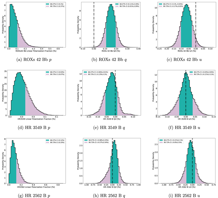
Figure 7. SPHERE targets: PDFs of the degree of linear polarization, Q/I, and U/I for each target with the 68.27% or 99.73% CIs indicated. Vertical dashed line indicates Q/I = 0 or U/I = 0.
Download figure:
Standard image High-resolution imageTable 4. Nondetection Polarization Limits
| Target | 68.27% Confidence Interval | 99.73% Confidence Interval | ||||
|---|---|---|---|---|---|---|
| p (One-sided) | q (Two-sided) | u (Two-sided) | p (One-sided) | q (Two-sided) | u (Two-sided) | |
| HD 4747 B | 0.14% | −0.16%, −0.04% | 0.00%, 0.08% | 0.25% | −0.25%, 0.10% | −0.08%, 0.14% |
| HR 7672 B | 0.10% | −0.10%, −0.04% | −0.00%, 0.06% | 0.23% | −0.23%, 0.02% | −0.11%, 0.10% |
| HD 19467 B | 0.55% | −0.16%, 0.54% | −0.35%, 0.32% | 1.25% | −0.94%, 1.14% | −0.81%, 1.12% |
| β Pic b | 0.18% | −0.12%, 0.12% | −0.05%, 0.16% | 0.37% | −0.34%, 0.34% | −0.24%, 0.30% |
| HR 3549 B | 0.06% | −0.06%, 0.01% | −0.04%, 0.04% | 0.14% | −0.13%, 0.10% | −0.11%, 0.11% |
| HR 2562 B | 0.26% | −0.08%, 0.23% | −0.20%, 0.10% | 0.67% | −0.59%, 0.52% | −0.60%, 0.48% |
| ROXs 42 Bb | 0.19% | 0.11%, 0.19% | −0.10%, −0.03% | 0.29% | 0.01%, 0.29% | −0.17%, 0.05% |
Download table as: ASCIITypeset image
6.1. HR 7672 B
After computing the S/N at the location of HR 7672 B as described above, we find S/NQ = 4 (and S/NU < 2.0) for both the combined 2018 data sets and the 2017 data set. Given this significant S/N at the location of the companion in Stokes Q, our task now is to decide whether the companion and stellar polarizations differ. If they are indistinguishable, we can conclude that an effect other than the intrinsic polarization of the companion is responsible for our S/N. We proceed by finding the distribution of Q and U values at the location of the companion using the approach described in Section 6. We compare these distributions with the stellar polarization calculated in Section 5 and listed in Table 2. The results are shown in Figures 8. We see that the companion and the star are indistinguishable in Stokes U, but their PDFs in Stokes Q hint at an offset between the companion and parent star. We note two important characteristics of Figure 8(a) and (c). First, in both epochs, the mean of the companion's PDF in Stokes Q is more negative than that of the host star—an encouraging sign for the interpretation that our signal is due to the intrinsic polarization of the companion. Second, in Figure 8(c), the mean of the star's PDF in Stokes Q is 6.0 standard deviations from zero. However, previous polarimetric observations of HR 7672 A show no such signal: Piirola et al. (2020) measure q = −4 × 10⁻⁴% and u = −4 × 10⁻⁴% using a broad bandpass of 400–800 nm. Per Serkowski's law of interstellar polarization, the polarization of HR 7672 A due to interstellar dust in our study's near-IR observations would be smaller still (Serkowski et al. 1975). Furthermore, the target's close proximity (17.71 pc; Bailer-Jones et al. 2018) disfavors polarization due to interstellar dust. We can therefore speculate that our observation of the star's nonzero polarization is due to uncorrected instrumental polarization on the order of 0.1% (Table 2).

Figure 8. Comparison of the polarization of HR 7672 A and B in two epochs of observation. Vertical dashed line indicates Q/I = 0 or U/I = 0.
Download figure:
Standard image High-resolution imageTo decide whether the companion's signal in Stokes Q significantly differs from that of the star (and hence differs from instrumental polarization), we mean-combine the two epochs of observation and subtract the mean-combined stellar distribution in Stokes Q from the mean-combined companion distribution in Stokes Q (we follow the same procedure for Stokes U). The results are shown in Figure 9. We find that the mean of the mean-combined, star-subtracted companion distribution in Stokes Q is located 2.1 standard deviations from zero while the mean-combined, star-subtracted companion distribution in Stokes U is located 0.75 standard deviations from zero.

Figure 9. Mean-combined star-subtracted HR 7672 B distributions in Stokes Q and U are consistent with zero to within 2.1 and 0.75 standard deviations, respectively.
Download figure:
Standard image High-resolution imageWhile not sufficient to claim a detection, these results encourages follow-up observations to determine whether HR 7672 B is intrinsically polarized. Under the assumption that we have not detected significant polarization from the companion, we can place limits on its Stokes Q, U, and degree of linear polarization values as in Section 6. The results are plotted in Figure 6 and tabulated in Table 4.
6.2. ROXs 42 Bb
We now return to our analysis of ROXs 42 Bb. Using the ring of comparison apertures, as described in Section 6, we obtain S/N > 20 at the location of the companion in Stokes Q and U for both dates of observation listed in Table 2. We also find that the flux observed from the stellar host is polarized (Table 2). There are several possible explanations for the host star's polarization: it could have a circumstellar disk; there may be magnetic star spots (e.g., Afram & Berdyugina 2015); or it could be polarized by the dichroic extinction induced by dust grains between the Earth and ROXs 42 B that are aligned with the local magnetic field. The spectral energy distribution of ROXs 42 B, however, shows no evidence of a circumstellar disk (Figure 10). Vrba et al. (1976) find stellar polarizations similar to that of ROXs 42 B in their observations of the Ophiuchus Cloud: Figure 11 shows their results with our observation of ROXs 42 B overplotted. While we cannot rule out magnetic starspots, these observations of the Ophiuchus Cloud indicate that interstellar dust is a source of the star's polarization. Our task now is to decide whether the companion's polarization significantly differs from that of its host star, and hence whether we have observed polarization due to the companion itself rather than interstellar dust.

Figure 10. This spectral energy distribution of ROXs 42 B shows that the observed photometry is in excellent agreement with the stellar synthetic spectrum, with no evidence of a disk at infrared or (sub)mm wavelengths. Blue circles show the observed photometry. Open circles are corrected for an extinction of AV = 1.7 mag (Bowler et al. 2014) using the reddening law from Fitzpatrick (1999), assuming a ratio of total to selective extinction of RV = 3.1. BT-Settl atmospheric models with Teff = 3700 ± 100 K and logg = 4.0 dex are shown in gray for comparison (Baraffe et al. 2015). Choice of physical parameters is based on the spectral type of M1 ± 1 for ROXs 42 B (Bowler et al. 2014). Conversion to effective temperature is based on Herczeg & Hillenbrand (2014). Inverted triangles represent upper limits. Photometry is from UCAC4 (B and V; Zacharias et al. 2013), USNO-A (R; Monet et al. 1998), 2MASS (J, H, and KS; Cutri et al. 2003), WISE (W1, W2,and W3; Cutri et al. 2012), Spitzer (3–24 μm; Evans et al. 2003). Upper limits at 0.88 mm and 1.3 mm are from Andrews & Williams (2007) and Wu et al. (2020), respectively.
Download figure:
Standard image High-resolution image
Figure 11. Reproduction of Plate VII in Vrba et al. (1976), showing stellar polarizations measured through the Ophiuchus Cloud. Length of each line is proportional to the star's degree of the linear polarization. Angle of each line indicates the degree of linear polarization (with p = 5% and χ = 90° indicated in the upper left). Our result for ROXs 42 B is plotted in red.
Download figure:
Standard image High-resolution imageUnlike the other companions in the survey, ROXs 42 Bb is bright compared to all starlight contributions at the same separation. Hence, we will use aperture photometry rather than negative companion injection to measure the flux of the companion in Stokes I. We select an aperture diameter of 5 pixels by maximizing the S/N at the location of the companion in total intensity. We find the preliminary distribution in Stokes I at the location of the planet by subtracting each comparison aperture sum from the planet's aperture sum. We estimate the PDF from this preliminary distribution using KDE.
In calculating the PDF at the planet's location in Stokes Q and U, we must also account for the photon noise of the bright companion (PNC). Following Perrin et al. (2015), we start by considering a single measurement of Q (or U) via double differencing:


where I+ and I− are the two orthogonally polarized channels, the numerical subscripts refer to different HWP positions, and  is the bias between the channels. Q is then given by

The variance in Q (or U) resulting from the PNC is therefore

where Ic,single represents the number of electrons inside the five-pixel diameter aperture at the location of the companion in one of the orthogonally polarized channels. Our final Stokes Q and U frames, however, are the average of n measurements of Q and U, where n is the number of HWP cycles. In terms of Ic, our measurement of the planet's signal in the final Stokes I frame, the variance at the companion's location in Q or U due to the photon noise of the companion is given by

where the factor of four accounts for (1) the fact that Stokes I includes twice as many frames as Q or U and (2) we are considering the signal in only one of the two orthogonally polarized channels.
To construct our final PDF in Stokes Q and U, we draw 106 samples from a Gaussian distribution whose mean is the aperture sum in Stokes Q or U at the companion's location and whose variance is given by Equation (7). As in Section 6, we find the distribution of the background at the companion's separation using a ring of comparison apertures and KDE. We draw 106 samples from this background distribution and subtract them from the samples drawn from the companion distribution. The resulting PDFs of Stokes Q/I and U/I at the companion's location are plotted in Figure 12. The PDFs of Stokes Q/I and U/I measured for the host star are also plotted in Figure 12 (Section 5).

Figure 12. Comparison of the polarization of ROXs 42 B and Bb in two epochs of observation.
Download figure:
Standard image High-resolution imageWe now average our PDFs of Stokes Q/I and U/I at the companion's location for the two dates of observation and subtract the similarly averaged host star PDFs. The results are plotted in Figure 14, and show that the mean-combined star-subtracted ROXs 42 Bb distributions in Stokes Q and U are separated from zero by 3.5σ and 1.7σ, respectively. This difference motivates follow-up observations to determine whether the companion's polarization is indeed different from that of its host star. However, with the information at hand, we cannot conclude that this difference is significant: the companion's Stokes Q/I and U/I PDFs have different widths depending on the date of observation, and the significance of the difference between the star and companion's Stokes Q/I PDFs is sensitive to the choice of aperture size and centroiding methods.
For the purposes of this paper, we will therefore proceed in placing an upper limit on the companion's degree of linear polarization, assuming that the host star and companion have been equally polarized by interstellar dust. It is worth noting that the polarization of the background star located approximately 05 from ROXs 42 B is consistent with this interpretation: following the same analysis as described above for ROXs 42 Bb, we find that the background star is somewhat more polarized than the ROXs 42 B system (Figure 13(a); this is consistent with its greater distance, as it is likely located behind the Ophiuchus Cloud) and its angle of linear polarization is similar to that of ROXs 42 B and ROXs 42 Bb (Figure 13(b)).

Figure 13. Comparison of the degree of linear polarization (a) and angle of linear polarization (b) between the host star ROXs 42 B, substellar companion ROXs 42 Bb, and nearby background star.
Download figure:
Standard image High-resolution imageContinuing with the assumption that the host star and companion have been equally polarized by interstellar dust, we compute an upper limit on the intrinsic polarization of the companion by considering the host-star-subtracted distributions in Figure 14. From these distributions, we compute the 68.27% and 99.73% confidence intervals as before. These are tabulated in Table 4 and indicated on the final histograms in Figure 7.

Figure 14. Mean-combined star-subtracted ROXs 42 Bb distributions in Stokes Q and U are separated from zero by 3.5σ and 1.7σ, respectively. Vertical dashed line indicates Q/I = 0 or U/I = 0.
Download figure:
Standard image High-resolution image7. Relating Linear Polarization to Projected Rotational Velocities
In this section, we relate the 68.27% CI upper limits on each companion's degree of linear polarization to the rotational velocity. For the purposes of this discussion, we assume an equatorial viewing angle (i.e., that v = v sin i). We will estimate each object's oblateness as a function of v, then compute the oblateness-induced degree of linear polarization as a function of v.
Following Sengupta & Marley (2010) and Barnes & Fortney (2003), we find the rotation-induced oblateness by way of the Darwin–Radau relationship:
where Rp and Re are the companions' polar and equatorial radii, Ω is the spin angular velocity, and g is the surface gravity. Finally, K = I/(MR2), where I is the companion's moment of inertia, M is the mass of the companion, and R is the radius of the companion.
We use the Sonora Bobcat evolutionary models for brown dwarfs and self-luminous exoplanets (M. S. Marley et al. 2020, in preparation) to relate the masses and ages given in Table 1 to the radii, surface gravities, and moments of inertia needed to calculate the oblateness using Equation (8). Compared with the evolutionary models published in Saumon & Marley (2008), the Sonora Bobcat models use different atmosphere models to find the surface boundary conditions (e.g., using improved opacities of H2, CH4 and alkali resonance lines) and include metals in the interior equation of state. These differences are described in M. S. Marley et al. (2020, in preparation).
Figure 15 shows the results. We find that our companions fall into three categories: (1) the young planetary-mass objects ROXs 42 Bb and β Pic b have the largest oblatenesses over the range of rotational velocities considered here; (2) HR 3549 B and HR 2562 B are intermediate-age, intermediate-mass brown dwarfs, and hence have intermediate oblatenesses; (3) HD 4747 B, HR 7672 B, and HD 19467B are old, higher-mass brown dwarfs, and hence have the lowest oblateness in our sample.

Figure 15. Median oblatenesses calculated for each target using Equation (8) and the parameters in Table 1.
Download figure:
Standard image High-resolution imageFor each target, we then compute self-consistent, homogeneously cloudy atmospheric models for the effective temperature and  values corresponding to the appropriate Sonora Bobcat evolutionary model. Previous studies of field brown dwarfs (e.g., Cushing et al. 2008; Stephens et al. 2009) have shown that typical L-type objects have cloud sedimentation efficiency fsed ∼ 2, and we adopt this value for our study. A larger value of fsed, with thinner clouds, would produce negligible polarization, while a smaller value, with more extended, optically thick clouds, would produce somewhat greater polarization. Given the observational limits and the uncertain values for the effective temperature and log (g) of each object, this intermediate, typical, value of fsed = 2 captures the cloud behavior without introducing an excessive number of parameters.
For each of these atmospheric models, we use the multiple scattering polarization code presented in Sengupta & Marley (2009, 2010) to compute the disk-integrated linear polarization fraction for each object as a function of oblateness and rotational velocity, assuming an equatorial viewing angle (i = 90°)—the viewing angle that gives the highest polarization fraction for objects with an oblate shape or patchy clouds. We assume that the disk-integrated polarization is due to oblateness alone. Figure 16 plots the linear polarization fractions as a function of the rotational velocity for each object in our sample, with the exception of HR 19467 B, which, as a T-dwarf, is not compatible with our cloud models. We note that the polarization of ROXs 42 Bb is not shown for rotational velocities greater than 79 km s−1, as this velocity corresponds to the planet's maximum possible oblateness value (f = 0.44).

Figure 16. Degree of linear polarization corresponding to most oblate models in Figure 15 and the 68.27% CI p upper limits calculated for each target.
Download figure:
Standard image High-resolution imageFigure 16 shows our 68.27% CI p upper limits and linear polarization models as a function of rotational velocity. An intersection of these curves constrains the companions' projected rotational velocities, assuming i = 90°. Panels (b) and (c) of that figure show that our 68.27% CI p upper limits are insufficient to constrain the rotational velocities of the brown dwarf companions in our sample. Improving our upper limits by a factor of three to five would be sufficient to constrain these objects' rotational velocity in a future survey.
Figure 16(a) shows that our upper limit is sufficient to constrain the rotational velocity of β Pic b, but not ROXs 42 Bb. For β Pic b, we find v < 68 km s−1. Of course, this object's rotational velocity has previously been measured using high-resolution spectroscopy: Snellen et al. (2014) measure v sin i = 25 ± 3 km s−1 for β Pic b. Similarly, Bryan et al. (2018) measure  km s−1 for ROXs 42 Bb. Using the same models used to produce the linear polarization fraction versus v values plotted in Figure 15(a), we conclude that the measured rotational velocities of ROXs 42 Bb and β Pic b would produce J- and H-band linear polarization fractions of p < 10−3%. Detecting such small polarization fractions with current instrumentation (GPI or SPHERE) would require significant improvements to our ability to subtract instrumental polarization and other instrument systematics (Wiktorowicz et al. 2014; van Holstein et al. 2020).
8. Conclusions and Future Work
We present a broadband near-IR polarimetric survey of two planetary-mass companions and five brown dwarf companions to nearby stars, finding that the degree of linear polarization is less than 0.6% (68.27% CI) for all targets. We relate our upper limits to models of linear polarization as a function of rotational velocity, and place these results in the context of previous measurements of these objects' spins using high-resolution spectroscopy.
It is the combination of such diverse techniques that will allow for new avenues of exoplanet characterization in the coming years. For example, Bryan et al. (2020) combined high-resolution spectroscopy with time-resolved photometry and astrometry to constrain the true obliquity of a planetary-mass companion outside of our own Solar System for the first time. However, the main limitation of this approach was the lack of any knowledge of the sky-projected spin–orbit angle; measurements of the oblateness-induced angle of polarization would address this limitation, allowing for a much tighter constraint on the true obliquity.
As planning for the next generation of ground and space-based observatories continues, it is crucial that we design our instruments to support these varied measurements. While the James Webb Space Telescope does not have polarimetric capabilities, the Roman Space Telescope (Akeson et al. 2019) Coronagraph Instrument has an imaging polarimetry mode that, for high-S/N targets, will measure the linear polarization fraction to <3% systematic accuracy at submicron wavelengths (e.g., Bailey et al. 2018). The next generation of ground-based giant segmented mirror telescopes (GSMTs), including the Thirty Meter Telescope (TMT), Giant Magellan Telescope (GMT), and Extremely Large Telescope (ELT), do not include AO-assisted polarimetric modes with <1% accuracy in their suite of first light instruments. Second-generation GSMT instruments dedicated to high-contrast imaging (e.g., TMT/PSI; Fitzgerald et al. 2019) provide an opportunity to study a wide range of exoplanets and substellar companions in polarized light. Ongoing upgrades to the GPI, SPHERE, and SCExAO adaptive optics systems, as well as a new coronagraphic polarimetry mode planned for Keck/NIRC2 (Ragland et al. 2019), offer near-term opportunities to study faint exoplanets in polarized thermal emission in the subpercent linear polarization regime.
This material is based upon work supported by the National Science Foundation under grant No. 1816920 and 1816341. R. J.-C. acknowledges the support of the The Miller Institute for Basic Research in Science at the University of California, Berkeley. The authors thank Marta L. Bryan for many useful conversations. The research of F. Snik and J. de Boer leading to these results has received funding from the European Research Council under ERC Starting Grant agreement 678194 (FALCONER). J. R. C. acknowledges support from the NASA Early Career Fellowship (NNX13AB03G) and NSF CAREER Fellowship (award #1654125) programs.
Facilities: Gemini(GPI) - , VLT(SPHERE). -
Software: astropy (Astropy Collaboration et al. 2013), VIP (Gomez Gonzalez et al. 2017), GPI Data Pipeline (Perrin et al. 2014), PyKLIP (Wang et al. 2015), IRDAP (van Holstein et al. 2020), emcee (Foreman-Mackey et al. 2013) SciPy (Virtanen et al. 2020).
Appendix: The Results of Negative Companion Injection Coupled with MCMC
The corner plots in Figures 17–22 show the posterior distributions corresponding to the parameters of the negative companions injected into each data set. The Stokes I frames before and after the negative companion injection are shown in Figures 23 and 24. See Section 4 for details.

Figure 17. HD 4747 B. (a) MJD = 8014.7. (b) MJD = 8341.8.
Download figure:
Standard image High-resolution image
Figure 18. HR 7672 B. (a) MJD = 8258.8. (b) MJD = 8342.6.
Download figure:
Standard image High-resolution image
Figure 19. β Pic b.
Download figure:
Standard image High-resolution image
Figure 20. HD 19467 B.
Download figure:
Standard image High-resolution image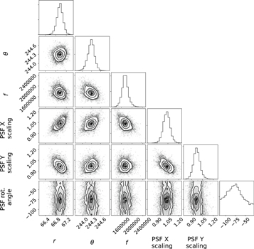
Figure 21. HR 3549 B.
Download figure:
Standard image High-resolution image
Figure 22. HR 2562 B.
Download figure:
Standard image High-resolution image
Figure 23. High-pass filtered Stokes I images of the brown dwarf companions and the sames images with the best-fit negative companion injected.
Download figure:
Standard image High-resolution image
Figure 24. PCA-reduced image of β Pictoris b, and the same image with best-fit negative companion injected.
Download figure:
Standard image High-resolution image