


Abstract
A prototype spectrograph using a Virtually Imaged Phased Array (VIPA) as the main dispersion element is presented, and its performance is fully examined in our laboratory. The single-mode, fiber-fed spectrograph with simultaneous wavelength calibration possesses a spectral resolution well in excess of  while the size of the VIPA is several orders of magnitude smaller than that of a conventional échelle with comparable resolution. In laboratory tests, the VIPA-based instrument with a homemade Yb:fiber ring laser frequency comb demonstrates a mode-to-mode tracking stability of 41 cm s−1 over a period of 6 hr. The VIPA spectrograph has promising applications in various astronomical observations in which ultra-high resolution and calibration precision are imperative, such as solar physics research, exoplanet searching with the radial velocity method, and O2 detection in the atmosphere of Earth-like planets. Ultimately, feasible optimizations for night-sky observations under seeing limited conditions are discussed.
Export citation and abstract BibTeX RIS

Original content from this work may be used under the terms of the Creative Commons Attribution 4.0 licence. Any further distribution of this work must maintain attribution to the author(s) and the title of the work, journal citation and DOI.
1. Introduction
Ultra-high-resolution spectrographs (UHRSs) with a spectral resolution  have been extensively utilized in modern astronomical research, such as the measurements of chemical abundances of the old solar twins (e.g., Monroe et al. 2013), isotopic ratios in stellar atmospheres (e.g., Knauth et al. 2003), and abundances of molecules in interstellar medium (e.g., Lauroesch et al. 2000), all of which are rather significant in tracking the Galactic evolution. It has become an indispensable tool in understanding the physics of stellar atmospheres, turbulence of the interstellar medium, and the structures of circumstellar disks and stellar winds. In particular, UHRSs with
  under seeing-limited conditions have been used in studies of interstellar and circumstellar matter (e.g., Crawford 1995; Price et al. 2001). Thanks to the long-term stability of the accurate wavelength calibration and stable point spread functions (PSFs), the UHRS is also a powerful facility for detecting periodic Doppler variations induced by substellar companions. It has been successfully applied in finding super-Earth planets (e.g., Mayor et al. 2011) and even Earth-mass planets (e.g., Pepe et al. 2013; Dumusque et al. 2014; Dressing et al. 2015) and is expected to play a central role in searching for habitable Earth-like planets around Sun-like stars (e.g., Fischer et al. 2016). The UHRSs equipped with very high-precision and long-term stable calibration sources are at work, for instance, the High Accuracy Radial velocity Planet Searcher (HARPS; Mayor et al. 2003) at the La Silla Observatory ESO 3.6 m telescope and the Echelle Spectrograph for Rocky Exoplanets and Stable Spectroscopic Observations (Pepe et al. 2010) at the ESO Very Large Telescope, and some are in construction.
So far, a series of simulation studies based on both photometry and spectroscopy has focused on the detectability of gaseous O2, a critical indicator of biosignatures in Earth analogs (e.g., Schneider 1994; Webb & Wormleaton 2001; Kaltenegger & Traub 2009), among which are UHRSs, combined with the cross-correlation technique and Doppler-shift analysis proposed by Snellen et al. (2013), which can feasibly detect O2 on next-generation ground-based Extremely Large Telescopes (ELTs). Very recently, López-Morales et al. (2019) suggested that the appropriate spectral resolution for O2 detection in the atmosphere of Earth-like planets should be  . Several proposals about such UHRSs have been put forward (López-Morales et al. 2019).
In solar physics research, UHRSs (usually  ) with a high spatial-resolution image system have been intensively employed to investigate the dynamic processes of the solar outer atmosphere and chromosphere (e.g., Morita et al. 2010; Wang et al. 2017), as well as fine structures and magnetoconvections (e.g., Watanabe et al. 2011; Wang et al. 2018). In addition, UHRSs with
  are also essential to retrieve the temperature and molecular abundance of the planetary atmosphere to clarify the interactions between the solar wind and the stratosphere of a planet, for example, Jupiter (Kostiuk et al. 1987).
Two categories of modern spectrographs may offer an ultra-high spectral resolution of  : (1) regular astronomical high-resolution spectrographs with échelle gratings as the main dispersion elements (e.g., Szentgyorgyi et al. 2012), and (2) spectrographs with externally dispersed interferometry (e.g., Erskine et al. 2016). Both of them have their own drawbacks: structural complexity and high costs for the former, extra telescope time for the latter. The Fourier-transform spectrometer, an interferometer working in the time domain, can also fulfill a very high spectral resolution. However, its low throughput at optical wavelengths restricts its applications in solar observations (e.g., Prieto & Lopez 1998). As a wavelength dispersion device, Virtually Imaged Phased Array (VIPA) has merits of structural simplicity, low price, and size compactness. It can provide excellent angular dispersion and low polarization sensitivity and thereby is particularly suitable to serve as the main dispersion element in UHRSs (e.g., Shirasaki 1996; Diddams et al. 2007; Fiore et al. 2016).
Another vital component of UHRSs is the wavelength calibration source. In this respect, the astrocombs offering a series of narrow, regularly spaced comb teeth in the frequency domain meet the criteria for ideal wavelength calibration sources (e.g., Steinmetz et al. 2008; Löhner-Böttcher et al. 2017). Generally, the astrocomb stabilized to either a Global Positioning System (GPS)-disciplined quartz oscillator (e.g., Doerr et al. 2012) or an atomic clock (e.g., Xu et al. 2017) can reach a stability of 10−12 in 1 s or even better for any length of time (Charsley et al. 2017). The solar spectrograph using an astrocomb as the calibration source has successfully attained the wavelength accuracy of 0.87 m s−1 and repeatability of 18.6 cm s−1 (Probst et al. 2015). In particular, ESO's HARPS northern counterpart, the HARPS-N spectrograph with an astrocomb calibrator, has achieved a 50 cm s−1 radial velocity (RV) rms over a few hours while observing the Sun as a star (Dumusque et al. 2015). Depending on the resolving power of the spectrographs (Murphy et al. 2007), the astrocomb usually demands a repetition rate of several dozens of gigahertz. Multiple stages of filtering cavities and optical amplifiers have therefore been adopted to enlarge the mode spacing of a laser frequency comb (LFC) whose repetition rate is smaller than 1 GHz and bring operational difficulties and measurement errors. Alternatively, a stabilized Fabry–Pérot etalon with stability better than 1 m s−1 in one night is a plausible and cost-effective calibration light source at least in the short and midterm (e.g., Cersullo et al. 2017). The richness of the Fabry–Pérot spectrum not only improves the wavelength calibration compared to the thorium–argon lamps but also extends the wavelength domain with respect to LFCs (Cersullo et al. 2019).
In this paper, we propose and implement a spectrograph with a VIPA as the spectral disperser and a homemade high-repetition-rate Yb:fiber LFC as the wavelength calibration source. The VIPA spectrograph offers an ultra-high spectral resolution and a precise wavelength calibration, as well as feasibility for controlling temperature and pressure due to its compact size.
This paper is organized as follows. In Section 2, we describe our instrumental method and present the preliminary results that will be further be analyzed in Section 3. The performance of the spectrograph including wavelength accuracy and repeatability, and the optimizations for night-sky observations under seeing-limited conditions are also discussed in this section. A summary is provided in Section 4.
2. Instrumental Setup
The top panel of Figure 1 shows the structure and dispersion principle of a VIPA, which has three regions of different reflectivities and can be viewed as a modified Fabry–Pérot etalon. The light is coupled into the VIPA via the bottom of the front side where an antireflective (AR) coating is used. The top of the front side with a high-reflective (HR with reflectivity r1) dielectric directs the light inside the VIPA toward the transmission direction. The rear side with a partially reflective coating (PR with reflectivity r2) transmits a small portion of light at each reflection point. Such design enables line-focused input light to enter the VIPA and undergo multiple reflections between the two sides, splitting the light into many paths. All of the transmitted light with a constant optical path difference between two adjacent waves generates the phased-array interference effect, resembling a diffraction grating (Shirasaki 1996; Xiao et al. 2004). VIPAs have been implanted in astronomical spectrographs as a high-dispersion element. Bourdarot et al. (2017) has reported a concept of a VIPA spectrometer with  (@653 nm) for monitoring young stars from a 6U Cubesat and demonstrated a laboratory prototype with
  . A proof of concept of a compact VIPA spectrometer with
  80,000, dedicated to the H and K bands, was being designed for the project "High-dispersion Coronograhy" developed at IPAG (Bourdarot et al. 2018), benefiting from its compactness and high resolving power.
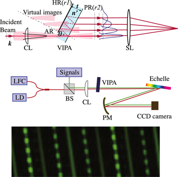
Figure 1. Top panel: the schematic of the VIPA spectral dispersion. Middle panel: the setup of the high-resolution spectrograph. The VIPA spectrograph illustrated above now fits on a 40 cm × 60 cm breadboard. CL: cylindrical lens, SL: spherical lens, LFC: laser frequency comb, LD: laser diode, BS: beam splitter, PM: parabolic mirror. Bottom: a partial raw image on a CCD of a flat-field light (lines) and simultaneous comb reference (dots) at wavelengths in the vicinity of 760 nm.
Download figure:
Standard image High-resolution imageThe VIPA used in the operational spectrograph is a commercial one purchased from LightMachinery Inc. (2020). It has a volume of 22 × 24 × 3.371 mm3 filled with fused silicon (nr = 1.46). The reflectivities are  and
and  in the working wavelength range of 680 to ∼800 nm, which is extendable with the coatings. The free spectral range (FSR) equals
  , dependent upon the refractive index nr, the thickness of the VIPA t, and the geometry of the spectrograph (θ, the angle of incidence at the VIPA). The resolving power of a VIPA reads (Hecht 2001)

where  is the center wavelength designed around 760 nm in our VIPA spectrograph. It theoretically predicts
  based on the above parameters, and the resolving power ranges feasibly from
  depending on the parameters, such as the HR and PR coating reflectivity, the materials, and the thickness.
The middle panel of Figure 1 shows the setup of our VIPA spectrograph fed with two channels of the signals and the wavelength calibration sources simultaneously via the single-mode fibers (SMFs). The VIPA acts as the main disperser with a cross-dispersed échelle grating, and a CCD camera constitutes the detecting part.
To suppress the high-order dispersion, both the cylindrical lens and the parabolic mirror have respective focal lengths of 500 and 516 mm. An off-the-shelf échelle grating (79.0 grooves mm−1, a blaze angle of 75°, and size of 25 × 50 mm2) is mounted orthogonally to the VIPA dispersion direction to separate the dispersion orders of the VIPA. The angle of incidence is  at the VIPA and 82
 5 at the échelle grating. A 14 bit, monochrome CCD camera is placed on the focus of the parabolic mirror to image the signals without external cooling system. The dark shot noise is 0.7 e- at room temperature for an exposure time of 100 milliseconds, and the read-out noise is 10 e- independent of exposure time. The CCD has a 5.5 μm pixel pitch with 2472 pixels in the dispersion direction of the VIPA and 3296 pixels in the dispersion direction of the échelle.
The application of SMFs to feed our UHRS improves the precision of the measurements efficiently. To track real-time drifts of the spectrograph precisely during the measurements, the UHRS is equipped with two fiber channels to calibrate the spectrograph simultaneously. The relative drifts between the two channels can be reduced by a rigid mechanical connection between the fiber inputs and subsequent light paths.
3. Characterization and Discussion
3.1. Resolution, Spectral Coverage, and Throughput
The bottom panel of Figure 1 shows a partial image of a flat-field white light with simultaneous comb references recorded by the CCD. The present parameters lead to the comb points being well Nyquist-sampled, and the average FWHM is around 5.4 pixels along the dispersion directions of both the VIPA and the échelle. The separation of signals from two channels is 18.88 pixels and distinguishable to some extent. The measured resolution of our spectrograph is  . Notable differences of the resolution between the theoretical and the experimental results originate primarily from the finite size of the VIPA. In contrast to the infinite dimension assumption in Equation (1), we take into account the interference from a finite number of waves in our simulations such that a resolution of
  is consistent with the experimental value results. On the other hand, the spectral range
  is approximately 4.9 nm wide, which is restrained by the detector size and can be improved significantly if necessary.
The reciprocal dispersion relationship of the VIPA can be derived as

which depends on the VIPA material (nr) and the angle of incidence on the VIPA ( ).
).
To be more concrete, we envisage a spectrograph using a customized VIPA with a resolution of  . Based on numerical calculations, such resolution requires a VIPA volume of 20 × 20 × 0.3 mm3 and an angle of incidence of 2°. According to Equation (2), the focus length of the camera
  mm ensures a five-pixel sampling of the resolution element if the pitch size of the CCD detector is 10 μm. If the cross-dispersion element is chosen properly and the order spacing is 10 × FWHM = 50 pixels, the wavelength range of 106 nm (wavelength center at 760 nm) can be covered with a detector of 1400 × 8000 pixels. Accordingly, a wavelength coverage of 458 nm (594–1052 nm) at
  is achievable with four VIPAs in parallel and a large-format detector (8000 × 8000 pixels). Fortunately, the four VIPAs are installed independently and bring no additional technical difficulties during the commissioning process.
The measured transmission of the VIPA is around 60%, which is comparable to a classical échelle grating and can be further optimized because the theoretical value of the transmission equals 78.76% for our VIPA according to the formula (Weiner 2012)

It should be noted that the cross-disperser is an échelle in the operational spectrograph. For practical utilization in future, especially for night astronomical observations, a ruled grating (e.g., 750 nm blaze, 1800 grooves per mm, 30 × 30 mm2 in Littrow configuration for the operational spectrograph) or a volume-phase holographic grating (Barden et al. 1998) is expected to perform the same dispersion capability to guarantee the higher efficiency. Moreover, the spectral scattered light accounts for 1.26% after averaging over the whole wavelength range.
3.2. Absolution Wavelength Calibration
Wavelength calibration is another key component of the spectrograph. Extremely high precision in wavelength calibration is indispensable in searching for exoplanets with the RV method. The tide is turning toward the LFC as the calibration light source for astronomical spectrographs. Our spectrograph is also equipped with a homemade Yb:fiber ring LFC as the wavelength calibration reference source. It has a repetition frequency (frep) of 810 MHz, which is sufficiently high for a spectrograph with spectral resolution  . Both the carrier-envelope-offset frequency (
 ) and frep are stabilized and referenced to a rubidium clock with a relative accuracy of about 10−11 in 1 s. More detail on the LFC can be found in Xu et al. (2017), Jiang et al. (2014). An external cavity laser diode (LD) with a superior thermal stability (
 /°C) and a narrow line width (<100 kHz) is used to calibrate the LFC modes. The LD working at the exact wavelength of 760.106870 nm is coupled into an SMF binding with the LFC light via the fiber coupler.
It is noteworthy that the VIPA interferometer demonstrates an Airy–Lorentzian line shape with respect to the output spatial intensity along the dispersion direction in the focal plane (Xiao et al. 2004). It is therefore inevitable to consider the influence of the line-shape characteristics of the VIPA on the wavelength calibration. In the present and next sections, the wavelength calibration of the VIPA spectrograph is investigated with the LFC spectral data using the reduction method following Probst (2015).
The absolute frequencies of the observed comb lines can be evaluated in terms of  , where
  MHz and
  have been defined precisely in our system. Then, the mode number n is determined by inspecting the LD and comb spectra as shown in the top panel of Figure 2. It is trivial to derive the mode number to be n = 486,923 in the present configuration as the spectrum of the LD is built up and superimposes on the comb mode corresponding to the wavelength 760.106941 nm.
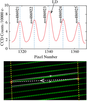
Figure 2. Top panel: the identification of comb mode numbers n. The graph shows the LD spectrum and a small fraction of the comb spectrum. The mode numbers n of the comb lines at the positions indicated by the blue dashed lines are derived from the known wavelength of the LD. Bottom: partial view of the spectrometer output consisting of the frequency comb modes and the LD.
Download figure:
Standard image High-resolution imageAnother key role of the narrow-line-width LD is to resolve the FSR of the VIPA. As shown in the bottom panel of Figure. 2, two noticeable bright points highlighted by red circles correspond to the LD in two consecutive orders of the VIPA. Two dashed yellow lines can be defined in such a way that they go through the two circles and are simultaneously vertical to the line connecting the two circles (dashed white line). Then, the modes located between the two dashed yellow lines are assigned to one FSR in each separate order of VIPA. The solid white lines with arrows indicate how the continuous modes are indexed and counted. It reveals that there are a total of 3145 observed comb lines conforming to the mode numbers ranging from 484,815 to 487,959 in a single measurement, corresponding to the wavelength range of 758.1 to 763.0 nm.
The line centers μ of different LFC modes are determined by fitting the comb line shapes using the Levenberg–Marquardt algorithm. The standard error of each line center σμ can be obtained from error propagation of the photon noise, which is assumed to be  , with N being the number of detected photoelectrons excluding the dark and bias currents of the CCD and R the CCD readout noise. The photon noise limit (PNL) is calculated using

where  is the Jacobian matrix and the weighting matrix
  is diagonal with
  (Gill & Murray 1978).
Here we fit the data with three different functions: Gaussian, Lorentzian, and hyperbolic secant with an additional linear term,
where x is the position on the detector within one of the VIPA orders and μ the expected position of the line center. The FWHM of the comb lines can be written as FWHM = 2.355σ, 2σ, and  for the Gaussian, Lorentzian, and hyperbolic secant functions, respectively.
The PNL values 0.65, 0.54, and 0.70 m s−1 are obtained for the three functions according to Equation (4), respectively. Data reductions of the astrocomb in échelle spectrographs (e.g., Wilken et al. 2012; Probst et al. 2015, 2016; Hao et al. 2018) have shown that the Gaussian function is a good approximation of the instrument's PSF. However, in our VIPA spectrograph with diffraction-limited input, the Lorentzian function is much better than the Gaussian or other fitting functions. This result may be attributable to the Lorentzian distribution of the PSFs in the VIPA spectrograph.
Absolute calibration is performed as a pixel-to-frequency relation by polynomial-fitting the line centers on the CCD as well as the known frequencies of the corresponding comb modes. The results are displayed in the top panel of Figure 3. A span of 53.18 m s−1 over an average CCD pixel is obtained from the fitted parameters. The rms deviation of the residuals fitted with a fifth-order polynomial after removing 3σ outliers is 1.49 m s−1 (middle panel of Figure 3), which cannot be significantly further improved by fitting with higher-order polynomials. The deviations of the comb line centers from the frequency solution in our case can be attributed dominantly to the dispersion characteristics of the VIPA itself. Both our simulation results following Xiao et al. (2004; see the bottom panel of Figure 3) and the experimental images show that the FWHMs of comb spectral lines vary gradually within one dispersive order of the VIPA. The spectral lines with larger FWHM will introduce more significant deviations in the data analysis. The quantile distribution of the residuals in the middle panel of Figure 3 clearly shows the residuals from the left-half side of the comb lines (blue) are larger than those from the right-half side (red). This indicates that the larger FWHMs of the comb lines will induce larger residuals. Furthermore, the overlap of the comb spectral lines and lower intensities of the comb teeth may also augment the errors. Because the FWHMs and the signal-noise ratios of the comb lines in one dispersive order of the VIPA have separate contributions to residuals, it is expected that the errors accumulated over whole spectral lines have non-Gaussian distributions.
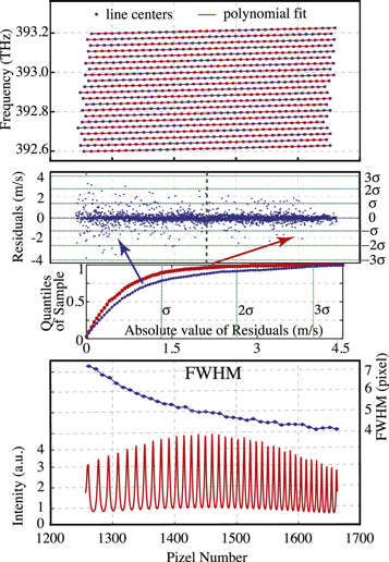
Figure 3. Top panel: frequencies of some of the observed comb modes vs. their line-center positions on the CCD. The data points are fitted by a fifth-order polynomial. Middle panel: the fifth-order polynomial fit residuals, converted to units of m s−1, and the quantile distribution of the residuals from the left (blue) and right (red). Bottom panel: simulation results of the LFC spectra dispersed by the VIPA in one FSR and the corresponding FWHMs of the comb lines.
Download figure:
Standard image High-resolution image3.3. Calibration Repeatability
Irregular spectral drifts are inevitable during the measurements due to the limited stability of the system, and so it is an essential process to examine the calibration repeatability of the system. The repeatability test of our spectrograph was carried out using two methods. The first is a two-channel simultaneous calibration (Probst et al. 2016), i.e., the light of the calibration source together with the LD signal is simultaneously sent to both channels A and B of the spectrograph. A number of subsequent acquisitions are recorded at equal intervals, and the first acquisition is assigned to be the reference acquisition (n = 0). The spectrograph drifts can be traced by the calibration shifts relative to the reference acquisition in both A and B, while the calibration precision of the spectrograph characterized by the calibration repeatability is derived from the relative shifts A−B. The averaged line shifts of acquisition n with respect to the reference acquisition 0 in units of RV m s−1 are calculated by considering the photon noise weighting as
where  and λi are obtained from the absolute calibration, and the weighting of (μni − μ0i) can be determined by

with  and
and  being the uncertainties of μni and μ0i which have been prepared in the line-position fittings.
In the process of subsequent acquisitions, the standard derivation (SD) of  denoted by σA–B quantifies the calibration repeatability of the spectrograph. In principle, it is expected that σA–B should approach the PNL
  when all noises are well suppressed except those of photons. From Equation (6),
  can be calculated as
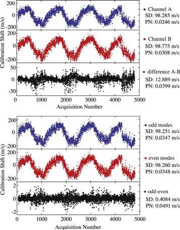
In the first test method, more than 4800 acquisitions were recorded every 5 s, and the recording time spans over 6.5 hr. The individual and relative shifts of the two channels (A and B) are shown in the top panel of Figure 4. The SDs of the two channels are both greater than 98 m s−1 (PNL: 0.0246 and 0.0308 m s−1), while the SD of the relative shifts amounts to 12.889 m s−1 (PNL: 0.0399 m s−1). Considerable drifts are expected in view of the fact that our spectrograph is sitting in an ambient condition with temperature fluctuations, air turbulence, and barometric pressure. In addition, the drifts between the two fiber inputs are inevitable even with the rigid mechanical connection. However, simultaneous calibration precision is not our major concern in this work. Here we focus on the data reduction method and the feasibility of simultaneous calibration on the VIPA spectrograph.
Figure 4. Top panel: tests of the calibration repeatability for a two-channel simultaneous calibration. The calibration shifts of two channels A (blue circles), B (red squares) and the relative shifts A−B (black asterisks) are compared. Bottom: tests of the calibration repeatability for odd–even comb mode number calibration. The calibration shifts of the odd modes (blue circles), even modes (red squares), and relative shifts odd−even (black asterisks) are compared. SD: standard deviation, PN: photon noise limit.
Download figure:
Standard image High-resolution image
We also notice that the channel drifts fluctuate periodically in phase with the ambient temperature, whereas the humidity and barometric pressure play minor roles. The relative shifts A−B are enhanced significantly at the individual drift valleys corresponding to temperature peaks, indicating that the temperature is a critical factor and influences the two channels independently. In spite of this, the above results confirm that simultaneous calibration is implemented successfully in our VIPA spectrograph. The long-term stability of the instrument will be improved prospectively, benefiting from such fiber-to-fiber tracking after the necessary environmental controls, in particular the temperature of the instrument.
We also examined the comb calibration repeatability with the scheme proposed by Probst et al. (2015) in which the comb modes in one channel were divided into two groups labeled by odd and even numbers. The SD of the relative shifts between the two groups evaluates the calibration repeatability, which incorporates random ingredients, such as photon noise, random spectral instability from comb teeth, part of the systemic errors, etc., and can measure the stability of the comb as the calibration source. The results of the odd and even modes and their difference are shown in the bottom panel of Figure 4. The SDs of the odd and even mode shifts are quantitatively consistent with those in the first method. Meanwhile, the SD of the relative shift is 0.4084 m s−1 (PNL 0.0491 m s−1). Similar to the case of the first method, the relative shifts have strong fluctuations at the temperature peaks. The SDs of the relative shifts in the short term (5 minutes) measured in the two methods are recorded as, respectively, 1.7612 and 0.1728 m s−1 in one of the most stable campaigns.
The repeatability of a two-channel simultaneous calibration quantifies the short-term drifts between subsequent acquisitions of the spectrograph. Deviations from the PNL of the relative shifts stem mostly from the instrumental drifts. Various mechanisms including the mechanical connection between the two-channel fiber inputs, environmental perturbations in the measurements, and random fluctuations in the comb-teeth intensity can result in uncertainties in the repeatability. On the other hand, the repeatability measured in the odd–even mode method is capable of eliminating the uncertainties from spectrograph drifts and characterizing the performance of the Yb:fiber ring LFC as the calibrator for UHRSs. If all of the error sources except photon noise are well suppressed, the SD of the relative shifts should be at the PNL level. However, our UHRS is neither evacuated nor temperature- and pressure-stabilized, the deviations in this case originate mainly from the beam perturbation caused by environment disturbance and the random variations of the comb-teeth intensity. For our instrument, it is apparent that the temperature is a key factor for the long-term stability of both the VIPA spectrograph and the LFC. Nevertheless, our experimental results verify that the VIPA spectrograph can make use of the LFC as an ideal calibration source.
3.4. Discussion
The VIPA spectrograph has shown its excellent performance in spectral resolution and wavelength calibration with the LFC under diffraction-limited conditions. It has potential applications in solar spectral research by virtue of the brightness of the Sun, which may be able to tolerate the relatively low efficiency of SMF couplings. Also, the highly precise Doppler velocities derived from the calibration precision may facilitate research at the solar convective blueshift and limb effect (e.g., Beckers & Nelson 1978; Balthasar 1984; de la Cruz Rodríguez et al. 2011), meridional motion (e.g., Dikpati & Gilman 2007; Doerr et al. 2012), and Sun-as-a-star RV measurements (e.g., Lagrange et al. 2010; Makarov 2010), etc.
All of the results presented in the previous sections are based on a spectrograph in diffraction-limited conditions. A challenging and appealing task is to apply the VIPA spectrograph to night-sky observation under seeing-limited conditions, such as exoplanet searching with the RV method and O2 detection in the atmosphere of an Earth-like planet. At present, most spectrographs are fed the starlight from telescopes via multimode fibers (MMFs) combined with the calibration source.
Now, we hypothesize a VIPA spectrograph with the MMF input of 100 μm core diameter, which corresponds to the seeing of 1'' on a 2 m  telescope. With other parameters intact, the resolution of
  requires the volume of the VIPA to be
  mm3 if the f numbers of the collimator and the camera are 10 and 10/3, respectively. The thicker the VIPA is, the smaller FSR will result. A wavelength range 70 nm can be covered by a single VIPA on a CCD detector with 1200 × 8000 pixels. Consequently, six VIPAs in parallel can lead to a wavelength coverage of 460 nm on a detector with 8000 × 8000 pixels.
As mentioned before, the resolving power is predominantly dependent on the thickness of a VIPA instead of its area, leaving the beam diameter unrestrained in the VIPA spectrograph. The small beam diameter can substantially reduce the volume of the components, for example, the collimator, making the spectrograph more compact and low cost. The total volume of such a VIPA spectrograph is estimated to be 60 × 60 × 30 cm3, facilitating the controls of temperature and pressure.
The existing astronomical spectrographs generally use échelle grating as the disperser, and the dependence of the spectral resolution on the field accepted by the fiber/slit ϕ and the telescope aperture D is given by (Pepe et al. 2000)

where h is the height of the échelle grating, and β is the grating's blaze angle. It is clear that to achieve an equivalent spectral resolution  , a larger échelle grating is required for a telescope with a larger aperture D. HARPS, a cross-dispersed échelle spectrograph (
 ), has the échelle size of
  mm3. Evidently, the manufacturing costs and technical difficulties of using the échelle will increase dramatically as the telescope diameter and spectral resolution increase, thereby restricting their applications. Following our previous discussion, the volume of a VIPA spectrograph with comparable performance is around 0.1 m3, much smaller than that of conventional échelle spectrographs. The compactness gives advantages in controlling the instrument temperature and pressure, and the long-term stability of the astronomical spectroscopic systems.
For current UHRSs, for example, the double-pass coudé spectrograph ( ) at the McDonald Observatory 2.7 m telescope and the Ultra-High-Resolution Facility (UHRF;
  ) at the Anglo-Australian Telescope (AAT), the total efficiencies, including sky and telescope transmission, slit loss, and spectrograph and CCD quantum efficiency, are smaller than 0.5%, and the wavelength coverage is merely a few angstroms (Ge et al. 2002). Such low throughputs primarily owe to the unique optics used to achieve the high resolving power in these instruments, namely a very narrow slit and double-path optics in the McDonald coudé 2.7 m telescope operated by the spectrograph and a confocal image slicer in the UHRF at the AAT. As a result, the current UHRSs at seeing-limited telescopes are generally restricted to the Sun and bright stars. For a spectrograph with a VIPA disperser of
  mm3, the simulations have shown that the resolving power attains
  even with a 50 μm core-diameter MMF input, thereby enhancing the efficiency greatly compared with conventional spectrographs.
The comb light couples into MMFs, inducing laser speckles and modal interference due to its high degree of coherence, so that uncertainties in the measurements may result. To diminish multipath interferences and the sensitivity to the light injection, Wilken et al. (2010) employed a dynamic mode scrambler to average over a large number of fiber modes. They achieved a short-term repeatability of Doppler shift 2.5 cm s−1 (Wilken et al. 2012). Moreover, Ye et al. (2016) coupled the comb light into an octagonal fiber by applying a dynamic agitation driven by a vibrator on the fiber to suppress the fiber noise and further tested it on the Chinese 2.16 m telescope at Xinglong Observatory, where a short-term repeatability of 0.1 m s−1 is realized (Hao et al. 2018). It is therefore quite viable to feed the VIPA spectrograph with MMFs by utilizing a scrambler mechanism to preserve the desired spectral resolution and wavelength calibration.
4. Summary
In this work, we put forward an ultra-high-resolution, LFC-calibrated VIPA spectrograph and fully examined its performance, such as the spectral resolution, wavelength calibration, and stability in the laboratory. Our design is particularly feasible for solar spectroscopic measurements. We also proposed some practical improvements on the VIPA spectrograph to extend our UHRS for night astronomical observations under seeing-limited conditions. With the resolving power ranging from 100 thousand to 2 million and the spectral coverage of several hundred nanometers, the VIPA spectrograph can be a useful complement to the astronomical échelle spectrograph.
The authors acknowledge support from the National Natural Science Foundation of China (grant Nos. 11773045, 11973009, and 11933005). J.H. thanks the CAS Pioneer Hundred Talents Program. The authors also thank Prof. Zhigang Zhang (PKU) for providing high-repetition-rate LFC technology and Prof. Dong Xiao (NIAOT, CAS) for helpful discussions.