


Abstract
To fully understand the diverse population of exoplanets, we must study their early lives within open clusters, the birthplace of most stars with masses >0.5M⊙ (including those currently in the field). Indeed, when we observe planets within clustered environments, we notice highly eccentric and odd systems that suggest the importance of dynamical pathways created by interactions with additional bodies (as in the case of HD 285507b). However, it has proven difficult to investigate these effects, as many current numerical solvers for the multi-scale N-body problem are simplified and limited in scope. To remedy this, we aim to create a physically complete computational solution to explore the role of stellar close encounters and interplanetary interactions in producing the observed exoplanet populations for both open cluster stars and field stars. We present a new code, Tycho, which employs a variety of different computational techniques, including multiple N-body integration methods, close encounter handling, modified Monte Carlo scattering experiments, and a variety of empirically informed initial conditions. We discuss the methodology in detail, and its implementation within the AMUSE software framework. Approximately 1% of our systems are promptly disrupted by star-star encounters contributing to the rogue planets occurrence rate. Additionally, we find that close encounters which that perturb long-period planets lead to 38.3% of solar-system-like planetary systems becoming long-term unstable.
Export citation and abstract BibTeX RIS
1. Introduction
The rate of exoplanet discoveries has exploded recently, fueled by new telescopes, technological advances, and increased interest among both astronomers and the general public. Discoveries of exoplanets in the Galactic field have dramatically outpaced discoveries in star clusters. This may be due to the limited number of stars observed by exoplanet surveys in star clusters, leading to an observational bias (Van Saders & Gaudi 2011). However, over the past several years, there have been a number of detections of planets in open star clusters, many with orbital parameters unlike what we see around field stars. As of this work's publication, there have been 34 planets observed within 10 Galactic open clusters. In Table 1 we catalog these planets and their parent clusters' relevant parameters. Additionally, Table 2 presents the measured parameters for the open clusters mentioned. From hot Jovians to eccentric Neptunes to volatile super-Earths, these exoplanets display the vast diversity of the planetary population. With new telescopes coming online and continued interest in exoplanet science, new discoveries of exoplanets around open cluster stars are inevitable.
Table 1. Parameters of Confirmed Exoplanets Located within Galactic Open Clusters
| Designation | M⋆ 
|
Mp 
|
Rp (RJ) | P (Days) | a (au) | e | References |
|---|---|---|---|---|---|---|---|
| Praesepe | |||||||
| Pr 0201 b | 1.24 ± 0.039 |

|
⋯ | 4.4264 ± 0.007 | ⋯ | 0.079 ± 0.078 | A |
| Pr 0211 b | 0.935 ± 0.013 | 1.88 ± 0.02 | ⋯ |

|
|
0.017 ± 0.01 | A |
| Pr 0211c | '' | 7.79 ± 0.33 | ⋯ |

|

|
0.71 ± 0.11 | B, C |
| K2-95 b | 0.44 ± 0.01 |

|
0.33 ± 0.018 | 10.1340 ± 0.0011 |

|

|
D, E |
| K2-100 b | 1.18 ± 0.09 |

|
0.31 ± 0.018 | 1.67391 ± 0.0011 | 0.0296 ± 0.0002 |

|
D, F |
| K2-101 b | 0.80 ± 0.06 | ⋯ | 0.18 ± 0.01 | 14.6773 ± 0.0008 | ⋯ |

|
D, F |
| K2-102 b | 0.77 ± 0.06 | ⋯ | 0.12 ± 0.01 | 9.91562 ± 0.0012 | ⋯ |

|
D, F |
| K2-103 b | 0.61 ± 0.02 | ⋯ |

|
21.1696 ± 0.0017 | ⋯ |

|
D, F |
| K2-104 b | 0.51 ± 0.02 | ⋯ |

|
1.97424 ± 0.0001 | ⋯ |

|
D, F |
| EPIC 211901114 b | 0.46 ± 0.02 | <5.0 |

|
1.64893 ± 0.0001 | ⋯ | ⋯ | D, F |
| Pr 0157 b | ∼0.9 | 9.49 ± 0.66 | ⋯ | 1234 ± 11 | ⋯ | 0.577 ± 0.023 | C |
| Hyades | |||||||
 Tau b Tau b |
2.7 ± 0.01 | 7.6 ± 0.2 | ⋯ | 549.9 ± 5.3 | 1.93 ± 0.03 | 0.151 ± 0.023 | G |
| HD 285507 b | 0.734 ± 0.034 | 9.17 ± 0.033 | ⋯ | 6.0881 ± 0.0018 | 0.0729 ± 0.003 | 0.086 ± 0.019 | H |
| K2-25/aV 50 b | 0.261 ± 0.021 | <1.15 |

|

|
⋯ |

|
I |
| K2-136 b | 0.74 ± 0.02 | ⋯ |

|

|
⋯ |

|
J |
| K2-136 c | '' | ⋯ |

|

|
⋯ |

|
J |
| K2-136 d | '' | ⋯ |

|

|
⋯ |

|
J |
| HD 283869 b | 0.74 ± 0.03 | ⋯ | 0.196 ± 0.13 |

|
⋯ | ⋯ | K |
| M67 | |||||||
| NGC 2682 YBP 1194 b | 1.01 ± 0.02 | 0.32 ± 0.03 | ⋯ | 6.959 ± 0.001 | ⋯ | 0.28 ± 0.08 | L |
| NGC 2682 YBP 1514 b | 0.96 ± 0.01 | 0.40 ± 0.38 | ⋯ | 4.087 ± 0.001 | ⋯ | 0.28 ± 0.09 | L |
| NGC 2682 SAND 364 b | 1.35 ± 0.05 | 1.57 ± 0.11 | ⋯ | 120.951 ± 0.453 | ⋯ | 0.35 ± 0.10 | L |
| NGC 2682 SAND 978 b | 1.37 ± 0.02 | 2.18 ± 0.17 | ⋯ | 511.21 ± 2.04 | ⋯ | 0.16 ± 0.07 | L |
| NGC 2682 YBP 401 b | 1.14 ± 0.02 | 0.42 ± 0.05 | ⋯ | 4.087 ± 0.007 | ⋯ | 0.16 ± 0.08 | M |
| Coma Berenices | |||||||
| CB 0036 b | ∼1.2 | 2.49 ± 0.10 | ⋯ |

|
⋯ |

|
C |
| CB 0036 c | '' |

|
⋯ |

|
⋯ |

|
C |
| NGC 6811 | |||||||
| Kepler-66 b | 1.038 ± 0.044 | ⋯ | 0.250 ± 0.014 |

|
0.1352 ± 0.0017 | ⋯ | N |
| Kepler-67 b | 0.865 ± 0.034 | ⋯ | 0.260 ± 0.014 |

|
0.1171 ± 0.0015 | ⋯ | N |
| Upper Scorpius | |||||||
| K2-33 b |

|

|
0.451 ± 0.033 | 5.42513 ± 0.0003 | 0.0409 ± 0.023 | ⋯ | O |
| 1RXS J16092105 b |

|

|
⋯ | ⋯ | <330 | ⋯ | P |
| GSC 6214-210 b | 0.83 ± 0.02 | 14.5 ± 2.0 | ⋯ | ⋯ | <320 | ⋯ | Q |
| Ruprecht | |||||||
| EPIC 219388192 b | 0.99 ± 0.05 | 36.5 ± 0.009 | 0.937 ± 0.042 | 5.2926 ± 2.6E−5 | 0.0593 ± 0.0029 | 0.193 ± 0.002 | R |
| NGC 4349 | |||||||
| 127 b | 3.81 ± 0.23 | ∼24.097 | ⋯ | 671.94 ± 5.32 | ∼2.35 | 0.046 ± 0.033 | S |
| NGC 2423 | |||||||
| 3 b | 2.26 ± 0.07 | ∼9.621 | ⋯ | 698.61 ± 2.72 | ∼2.02 | 0.088 ± 0.041 | S |
| IC 4651 | |||||||
| 9122 b | 2.06 ± 0.09 | ∼7.202 | ⋯ | 747.22 ± 2.95 | ∼2.05 | 0.150 ± 0.068 | T |
Note. The above columns are as follows: the host star's mass, M⋆; the planet's mass (or  ), Mp; the planet's radius, Rp; the orbital period, P; the orbital semimajor axis, a; orbital eccentricity. Due to the limitations of different detection methods and the differences in stellar magnitude sensitivity in surveys, some planets currently do not have certain parameters measured. Predictions and upper bounds have been provided where possible. This collection has been drawn from the following sources: the Extrasolar Planets Encyclopaedia (exoplanet.eu); the NASA Exoplanet Archive; and the Open Exoplanet Catalog (Rein 2012, www.openexoplanetcatalogue.com).
References. A (Quinn et al. 2012), B (Malavolta et al. 2016), C (Quinn 2016), D (Obermeier et al. 2016), E (Mann et al. 2017a), F (Stefansson et al. 2018), G (Sato et al. 2007), H (Quinn et al. 2014), I (David et al. 2016a; Mann et al. 2016a), J (Livingston et al. 2017; Mann et al. 2017b), K (Vanderburg et al. 2018), L (Brucalassi et al. 2014), M (Brucalassi et al. 2016), N (Meibom et al. 2013), O (David et al. 2016b; Mann et al. 2016b), P (Lafrenière et al. 2008, 2010), Q (Ireland et al. 2011; Pearce et al. 2018), R (Nowak et al. 2017), S (Lovis & Mayor 2007), T (Mena et al. 2018).
Download table as: ASCIITypeset image
Table 2. Parameters of Open Clusters with Detected Exoplanets
| Designation | MT 
|
tage (Myr) | D⊙ (kpc) | Rc (pc) | RT (pc) | [Fe/H] |
|---|---|---|---|---|---|---|
| Hyades | ∼400 | 625 ± 50 | 0.04634 ± 0.0003 | ∼2.7 | ∼10.3 | +0.146 ± 0.004 |
| Praesepe/NGC 2632 | 511 ± 73 | 830 | ∼0.187 | ∼3.5 | ∼12 | +0.156 ± 0.004 |
| M67/NGC 2682 |

|
3550 | 0.841 ± 0.048 | 0.60 ± 0.06 | 4.13 ± 0.43 | +0.050 ± 0.040 |
| Coma Berenices/Melotte 111 | 112 ± 16 | 690 | ∼0.087 | 6.80 ± 0.30 |

|
+0.070 ± 0.090 |
| NGC 6811 | 144 ± 32 | 710 | 1.460 ± 0.086 | 0.36 ± 0.04 | 2.89 ± 0.42 | −0.500 ± 0.200 |
| Upper Scorpius/Sco OB2-2 | ∼2060 | 11 ± 2 | ∼0.145 | ∼28 | ∼50 | ⋯ |
| Ruprecht 147 | 58.88 ± 1.45 | 2140 | 0.295 ± 0.015 | 6.51 ± 3.78 | 6.76 ± 0.97 | +0.070 ± 0.030 |
| NGC 4349 | 1654 ± 199 | 710 | 1.430 ± 0.085 | 0.64 ± 0.09 | 3.68 ± 0.58 | +0.105 ± 0.108 |
| NGC 2423 | 120 ± 30 | 1000 | 0.756 ± 0.044 | 0.18 ± 0.03 | 1.23 ± 0.20 | +0.068 ± 0.103 |
| IC 4651/Melotte 169 | 1443 ± 277 | 1410 | 1.006 ± 0.059 | 0.70 ± 0.11 | 3.48 ± 0.36 | −0.128 ± 0.082 |
Note. The above columns are as follows: total cluster mass, MT; estimated age from isochrone fits, tage; distance from the Sun to the cluster's core, Dodot; the core radius, Rc; the tidal radius, RT; metallicity of the cluster compared to the solar standard, [Fe/H]. The most recent measurements for each parameter have been recorded in this table assuming the values agree with the guidelines laid out in Netopil et al. (2015).
References. Hyades (Perryman et al. 1997; Cummings et al. 2017), Praesepe (Adams et al. 2002; Kharchenko et al. 2013; Cummings et al. 2017), M67 (Bukowiecki et al. 2011; Kharchenko et al. 2013; Geller et al. 2015; Overbeek et al. 2016), NGC 4349, NGC 2423, and IC 4651 (Bukowiecki et al. 2011; Kharchenko et al. 2013), Coma Berenices (Casewell et al. 2006; Kraus & Hillenbrand 2007; Melnikov & Eislöffel 2012; Kharchenko et al. 2013; Joshi et al. 2016), NGC 6811 (Bukowiecki et al. 2011), Upper Scorpius (de Zeeuw et al. 1999; Preibisch & Mamajek 2008; Pecaut et al. 2012; Donaldson et al. 2017), and Ruprecht 147 (Curtis et al. 2013; Kharchenko et al. 2013; Joshi et al. 2016).
Download table as: ASCIITypeset image
Most stars with masses >0.5M⊙ were likely born in clustered environments; a substantial fraction of these natal clusters have since dissolved in the Galactic tidal field (Lada 2010; Portegies Zwart et al. 2010; Fujii & Portegies Zwart 2016). Therefore, many planetary systems currently observed in the Galactic field were likely born in significantly denser environments. Fully understanding the origins of the orbital properties of exoplanet systems will require a detailed study of their dynamical histories from their birth cluster onward. Modeling the dynamics of planetary systems in star clusters is a complex problem, largely due to the very different timescales involved, beginning with planetary orbits of order days through stellar orbits throughout the cluster of order megayears. In this paper we develop the modeling tools needed to accomplish this task.
Coupling planetary orbit evolution and cluster dynamics is a complex multi-scale problem that cannot be efficiently solved using conventional numerical methods. Previous studies have used direct N-body calculations (Spurzem et al. 2009; Cai et al. 2016, 2017, 2018), Monte Carlo schemes for modeling close encounters (Hao et al. 2013), and simulating gravitational potential perturbations on planetary systems from the cluster (Cai et al. 2014; Wang et al. 2020). Direct N-body calculations can be computationally costly and may pose scaling problems when applied to large systems (Aarseth 2003). Monte Carlo approaches to simulating the close encounter histories of a system are fast, but may not adequately represent conditions in clusters with small N, like the open clusters we are interested in here (Fregeau et al. 2003; Giersz et al. 2013). Linking the gravitational potential of a cluster to separate simulations of the planetary systems running in parallel, while highly accurate, can only be implemented for short cluster lifetimes due to computational limitations. Therefore, a numerical method that allows for the accurate determination of cluster dynamics and planetary orbital evolution over long time periods (comparable to the dissolving time of an open cluster) with low computational overhead is required.
In this paper we describe such an implemented methodology, called Tycho, and provide proof-of-concept results. In Section 2 we discuss Tycho's implementation within the AMUSE software framework (Portegies Zwart & McMillan 2018).5 In Section 3, we detail our chosen initial conditions, which draw heavily from recent empirical studies. In Sections 4 and 5, we explore some representative results of production runs illustrating Tycho's current capabilities.
2. Methodology
In this section, we describe in detail the methods used in Tycho. In short, we record the close encounter histories of stars via direct N-body simulations of clusters, which inform a series of scattering experiments on multi-planet systems contained within the cluster. Utilizing multiple independently verified integrators and packages, the result is a robust method for accurately studying the change of planetary systems due to all dynamical effects present in such environments. For a visual depiction of our methodology, see Figure 1.

Figure 1. Flow chart of the general processes involved in the Tycho simulation pipeline.
Download figure:
Standard image High-resolution image2.1. Modeling the Cluster's N-body Dynamics
Cluster-scale gravitational dynamics is handled by PH4, an MPI-parallel fourth-order Hermite direct N-body integrator with GPU acceleration (McMillan et al. 2011). This AMUSE module is well tested on N-body systems of all sizes, from binaries to clusters containing hundreds of thousands of stars (see Portegies Zwart & McMillan 2018). Like most N-body integrators in AMUSE, PH4 does not include any special treatment of close encounters between stars or binaries. Most AMUSE modules, including PH4, include the possibility of softening the potential, but this is not appropriate for the collisional dynamics of interest here. Instead, Tycho uses the AMUSE Multiples module to manage dynamical close encounters (Pelupessy et al. 2013; Portegies Zwart & McMillan 2018), as we now describe.
Traditional collisional N-body codes devote a substantial fraction of the total code base to modeling the detailed internal motion of multiple systems (where this term henceforth includes stellar binaries) simultaneously with the large-scale motion of the rest of the system (Portegies Zwart et al. 1998; Aarseth 2003). The algorithms involved have varying degrees of efficiency and accuracy, but all gradually relax the accuracy of the perturbed binary integration until "unperturbed" binaries (where the external tidal acceleration is less than ∼10−6 times any internal acceleration) are treated as isolated unperturbed objects. The alternative approach, widely used in Monte Carlo schemes, treats stable multiples as completely unperturbed until they interact strongly with another object (Fregeau et al. 2004; Tanikawa & Fukushige 2009; Giersz et al. 2013).
As discussed in more detail by Portegies Zwart & McMillan (2018, Section 4.5) the N-body module (here PH4) manages a multiple's center of mass, but is ignorant of its internal dynamics. The Multiples module maintains a database of all stable multiples in the system. Herein, we define that a stable multiple is a binary, a hierarchical triple deemed stable by the Mardling (2007) criterion, or a higher-order multiple system in which the Mardling criterion applied to the outermost orbit(s) indicates approximate stability. Each single or multiple object has an interaction radius Rint assigned to it. For a single star of mass M, Rint ∼ GM/σ2, where σ is the cluster velocity dispersion. For a multiple, Rint is twice the outer semimajor axis. For planets, Rint is the Hill radius when bound to a star, and  when free-floating. When two particles in the N-body code approach within the sum of their interaction radii, the N-body integrator is advanced to and paused at that moment. The particles are then removed from the N-body system, their internal structure is restored, and the interaction is followed as an isolated few-body system using the SmallN integrator, a robust shared-step, time-symmetrized code with analytic extensions (Hut et al. 1995; McMillan & Hut 1996; Portegies Zwart & McMillan 2018). Pure two-body encounters are advanced analytically using the AMUSE Kepler module.
In order to inform the high-fidelity scattering experiments detailed in Section 2.4, we store the encounter history of each star throughout the course of the simulation. At the start of a close encounter, Tycho copies the flattened hierarchical tree of the root particles involved into an AMUSE particle set. This particle set and all required initial conditions are then stored in a chronological database of encounter histories for each star in the simulation. Once the N-body evolution ends, a complete history of all stellar close encounters is available within the database.
The structure of the few-body system is monitored during the SmallN integration and the integration is declared over when the system consists of some number of mutually unbound, receding, stable (as just defined) centers of mass. For stars with planetary systems, the "over" criterion is applied only to the stars. At that point, the internal structure of the newly obtained multiples is stored for future use, corrections are applied to partially account for the tidal field of the rest of the N-body system, the centers of mass are added to the N-body system, and the large-scale integration continues. The internal structure of each center of mass particle is held static until the next interaction occurs. Examples of this hierarchical structure can be found in Figure 2.

Figure 2. Typical hierarchical system in our simulations. Multiples handles such systems by grouping nearest bound neighbors in a tree structure, storing all particle information at each level. This process continues until there are no further bound pairs. Not shown here is the fact that the leaves of the tree can themselves be roots of their own trees.
Download figure:
Standard image High-resolution image2.2. Stellar Evolution
For our models, all primary stellar masses are drawn from a Kroupa (2001) mass function, as discussed in detail in Section 3.1. In addition, we include primordial binaries and allow dynamical binaries to form naturally, to ensure an accurate depiction of large-scale cluster dynamics. Tycho uses the SeBa stellar evolution module (with solar metallicity), with an additional prescription for mass loss due to winds (Portegies Zwart & Verbunt 1996, 2012; Toonen et al. 2012).
To account for multiple age groups in our stellar population, we implement a procedure for asynchronous evolution within SeBa. This methodology will become increasingly more important for accurate depictions of dynamics as direct simulations of cluster formation from molecular clouds become more widespread (e.g., Wall 2018; Wall et al. 2019). In order to accomplish this, we bin our stars by their age, which allows us to create separate instances of SeBa for each grouping. These separate instances within the AMUSE environment allow for the module to accurately evolve while reducing the computational overhead to a manageable level. See Figure 3 for an example of a Hertzsprung–Russell diagram drawn from a roughly 500 M⊙ cluster.

Figure 3. Hertzsprung–Russell diagram for a ∼350M⊙ (∼675 stars) cluster at various epochs. Each point represents an individual star whether or not the star is part of a close hierarchical system. By 1.5 Gyr, we have lost ∼50M⊙ to stellar evolution and supernovae.
Download figure:
Standard image High-resolution image2.3. The Background Galactic Potential
The evolution of a cluster within the tidal field of its host galaxy is substantially different from one in isolation. The tidal field imposes a limiting Jacobi radius on the cluster, at which stars become unbound (von Hoerner 1957; King 1962). As mass is lost from the cluster, the radius shrinks, leading to a decreased cluster lifetime (Baumgardt & Makino 2003; Gieles & Baumgardt 2008). In order to accurately model the escape of stars from the cluster into the Galactic field, we apply a background gravitational potential which models key aspects of the the Milky Way. As described in detail in Bovy (2015), this static potential features a central bulge, a dusty disk and a dark matter halo modeled after current Milky Way observations. To couple the Galactic potential with the time-dependent evolution of the cluster, we utilize the AMUSE framework's Bridge package, a code-coupling algorithm based on the scheme described by Fujii et al. (2007). A cluster may be placed in any kind of orbit in this potential and the relevant tidal forces will be fully taken into effect.
2.4. Handling Planetary Dynamics on Different Scales
Of the 4126 confirmed exoplanets to date, 1766 exist within 705 multi-planetary systems.6 Accordingly, it is critical to include within Tycho the ability to faithfully model multi-planet systems. In our model, we record the parameters of all close encounters between stellar systems (single or hierarchical) in the cluster and use these parameters to later perform a series of scattering experiments, the procedure for which we will now describe.
Once the full-cluster N-body simulations are completed, we re-simulate our independent encounters in parallel at higher temporal resolution with additional planetary bodies drawn from our mock solar system model described in Section 3.2. We again utilize the specialized few-body integrator SmallN for these scattering experiments. To improve run-time efficiency, we advance the two stellar systems involved in the encounter along their Keplerian orbit to the point, r12, where the gravitational perturbation on the outermost orbit is of order 10−3:

Here aouter is the semimajor axis of the outermost planet, Mpert is the total mass of the perturbing system, and Mhost is the mass of the star hosting the planetary system. We then allow SmallN to simulate the close encounter utilizing an adaptive internal time step, storing particle position and velocity vectors every 1 yr until the close encounter is declared over, as described in Section 2.1. We then evolve the system for an additional 100 yr before committing and tabulating the planets' orbital parameters.
To ensure that our dynamical parameters are fully sampled, we simulate each encounter in our database with the host star's planetary system multiple times, with different orientations and mean anomalies. At the start of each scattering experiment instance, we apply a random rotation transformation which samples the unit sphere uniformly to the system using the fast algorithm developed by Arvo (1992). The proof of this method's uniform coverage is outlined by Shoemake (1992). To develop a statistically significant population of encounters from our N-body database, we repeat this procedure 100 times.
2.5. Determining Long-term Stability of Planetary Systems
As we are interested in the evolution of our systems over their time spent within the parent cluster, we need a quantifiable system for analyzing not only the shifts in a given planet's orbits, but also the overall stability of the system they inhabit. Measuring the angular momentum deficit (AMD) in our systems allows for such a metric. Following Laskar (1997), the ratio of a planet's relative AMD to that of its system as a whole can be interpreted as a secular measure of the perturbation of the orbit. We can then find the regime in which the possibility of strong encounters with other bodies in the planetary system are forbidden, implying long-term stability.
Due to its conservative nature, many different stability criteria can be included into the AMD framework. For our purposes, we specifically include the criteria imposed on the critical AMD (the value at which a given planet becomes unstable) stemming from Hill stability (Petit et al. 2018), orbit-crossing collisions (Laskar & Petit 2017), and first-order mean motion resonance (MMR) overlap (Petit et al. 2017). We present a complete summary of the AMD framework in the Appendix.
In order to allow for an efficient and complete classification of our planetary systems, we adopt the following prescription: if the jth planet's AMD-stability coefficient  , we do not calculate Cc; if the reverse is true, then we set
  . As noted in Section 4 of Petit et al. (2018), this ensures the system's long-term stability or lack thereof is correctly validated. Using βj as a post-processing indicator, we are able to correctly categorize our systems as stable (where all planets have βj < 1), unstable (where two or more planets have βj > 1), or metastable (where the innermost planet is unstable but all other planets are stable).
3. Tycho's Initial Conditions
Tycho aims to provide a physically accurate depiction to the evolution of planetary systems embedded within stellar clusters. In the following subsections, we describe our specific initial conditions for this project. However, we note that these can be readily modified to suit other needs; Tycho is at its core built to be a versatile tool for modeling the effects of stellar cluster dynamics on multiple scales. To ensure that our simulations can be compared with statistics drawn from observational surveys, our initial conditions are drawn from empirical data while allowing some room for well-constrained, fixed parameters.
3.1. Stars and Primordial Binaries
We draw our clusters' spatial density distributions from King (1962, 1965, 1966) models, which provide rudimentary, if imperfect, fits to observed stellar clusters with masses of a few times 103M⊙ (Portegies Zwart et al. 2010). Detailed observations of star-forming regions show stellar distributions which tend to be clumpier in composition than King models (Sánchez & Alfaro 2009; Allison et al. 2010), with stars still embedded in their natal gas for the first few megayears. N-body models of hierarchical or fractal stellar clusters relax to King-like spatial distributions in a short time (Geller et al. 2013; Smith et al. 2013). We synthetically age our stellar population and begin our models at 10 Myr, to avoid this gas-embedded, spatially clumpy phase. In the future, we will couple our models to detailed star formation simulations (such as those presented in Wall et al. 2019) to better capture this initial phase. For convenience, we initialize all of our clusters on circular orbits of Galactocentric radii 9 kpc.7
For our stellar masses, we sample a truncated Kroupa initial mass function (IMF; Kroupa 2001). We set our lower and upper stellar mass limits as the lowest mass for an observed red dwarf (Mmin = 0.1M⊙; Dieterich et al. 2014) and the approximate maximum single-component mass following complete gas ejection at ∼5–10 Myr (Mmax = 10M⊙; Lada 2010), respectively. Limiting our lower mass allows for us to more efficiently spend computational resources integrating the cluster's evolution, without significantly altering the overall evolution of the cluster (Kouwenhoven et al. 2014).
We draw the orbital parameters of our primordial stellar binary population from empirical distributions derived from observational surveys. The creation procedure implemented is as follows.
- 1.To determine if a given primary star should have a stellar binary companion, we adopt the empirical binary fractions as a function of primary mass from Figure 12 of Raghavan et al. (2010). If a star is selected to have a secondary component, its position becomes the center of mass of the new binary.
- 2.The secondary mass is selected from the truncated Kroupa IMF and added to the initial mass of the center of mass particle. This allows us to recover the observed IMF when we redistribute the mass between the primary and secondary star.
- 3.
- 4.To determine the stellar binary's orbital elements, we use the primary's mass to draw from empirically based distributions. The period is generated from the log-normal distribution of Raghavan et al. (2010) for lower-mass and Sana et al. (2012) for higher-mass systems. Eccentricities are drawn from a uniform distribution well documented in the literature (Raghavan et al. 2010; Duchêne & Kraus 2013; Moe & Di Stefano 2017).
- 5.The orientation of the system with respect to the cluster's coordinate system is chosen randomly and uniformly over the unit sphere as described in Arvo (1992).
Figure 4 provides an overview of the yield of the above-described procedure. Once generated, binaries are added to the N-body particle set to be picked up by Multiples before the cluster is scaled to virial equilibrium. All internal orbital interactions, close encounters, and stellar evolution are tracked and stored by Tycho's bookkeeping procedures for future analysis. There are no initial systems consisting of more than two bodies in our simulated clusters.

Figure 4. Initial conditions for our primordial binary population, for a sample of 100,000 binaries. Left: reconstruction of the orbital distributions presented in Raghavan et al. (2010) and Marks et al. (2011) for young clusters. Note that orbits shorter than ∼10 days are assumed to be circularized due to tidal effects. Right: reconstruction of the binary mass ratio, q. Note that the lower probability for small q in M-type stars is due to our minimum partner mass criterion, as we treat stars separately from brown dwarfs/planets.
Download figure:
Standard image High-resolution image3.2. Planetary Systems
Within the initial cluster models presented in the previous section, we model the planetary systems after our own solar system—using a stable, well-studied system allows us to differentiate the effects of star–star scattering on multi-planet systems from internal interplanetary dynamics. Thus we adopt a scaled version of the solar system, which contains only analogs for Earth, Jupiter, and Neptune. We refer to these as Terrestrial, Jovian, and Neptunian, respectively. We initialize our systems as coplanar, consistent with leading formation models (Laskar 2000).
In accordance with current formation theory, the placement of each system's Jovian is scaled to the snow line of its host star (Kennedy & Kenyon 2008). Thus, the Jovian planets have semimajor axes  (Ida & Lin 2005). After scaling the Jovian's semimajor axis, we scale the other planetary orbits so that the system remains long-term stable. By fixing the ratio of periods between each planet and the system's Jovian, we ensure that the solar system's innate stability is preserved regardless of the mass of the host star. A good measure of this is the AMD of the planets (see Section 2.5). Table 3 summarizes our model's parameters and provides the AMD stability coefficient of each planet, averaged over the host star masses in our simulations.
Table 3. Implemented Planetary Systems
| Mass (MJ) | Eccentricity | Semi-major Axis (au) | Avg. AMD Stability Coefficient, 
|
|
|---|---|---|---|---|
| Terrestrial | 0.003 | 0.016 |

|
|
| Jovian | 1 | 0.048 |

|
(0.2394 ± 2.35) × 10−4 |
| Neptunian | 0.054 | 0.009 |

|
(0.02361 ± 1.79) × 10−5 |
Download table as: ASCIITypeset image
4. Proof-of-concept Simulations
4.1. Experimental Setup
To illustrate our improved approach for simulating planetary systems within clusters, we simulate 40 independently seeded open clusters with initial conditions as described above. These consist of 10 realizations for each of the possible parameter combinations of the number of center-of-mass objects (N ∈ {100, 1000}) and the depth of the King potential (W0 ∈ {3.0, 6.0}).8 Each realization is simulated according to our prescription for approximately 2 Gyr, which is past the point of cluster dissolution in most cases. Planetary systems are generated only around single stars and include only the Jovians in our full-cluster N-body simulations (as discussed above), but we retain the full planetary systems in our scattering experiments. For the purposes of showcasing the dynamics, we limit our close encounter database to those with rperiapsis < 2aouter.
Our simulations were performed on the Draco supercomputing cluster at Drexel University. Draco consists of 24 compute nodes, each consisting of two Intel Xeon x5650 CPU six-core chips and four to six vintage (Tesla/Titan) NVIDIA GPUs, allowing us to take advantage of PH4's parallel and cuda-enabled design. Our N-body simulations took 553 CPU hours to complete, and our scattering experiments took 1690 CPU hours, for a total of 1.33 weeks distributed across 10 nodes.
4.2. Results
A catalog of our simulations has been provided to the publisher, containing a total of 41,313 planetary systems of various configurations. Figure 5 shows the relation between the total change in eccentricity and the total change in semimajor axis for our three planetary populations after cluster dissolution. Most of our stellar population only encountered another stellar system once over the 2 Gyr evolution. Given the much greater scattering cross section of our Neptunian population, our results confirm the expectation that they are far more significantly affected by stellar flybys than the Jovian or Terrestrial planets. Indeed, of the 371 planets that escaped their host system across all encounters, 222 were Neptunians, 77 were Jovians, and 61 were Terrestrials. Further, of these planets that left their systems, the Neptunians were more likely to be captured (26 Neptunians versus fove Jovians and no Terrestrials).
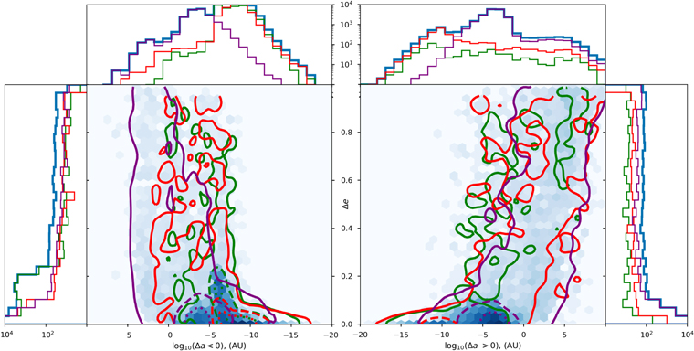
Figure 5. Total change in orbital elements a and e of exoplanets at the point of their host star's ejection from the cluster. The background hexagon-binned histogram is the total for all planets and the contours represent the three planetary populations: green for Terrestrials, red for Jovians, and purple for Neptunians. Dotted lines represent the contour containing greater than 100 counts; dashed lines represent the contour containing greater than 10 counts, and solid lines represent the contour containing greater than one count.(The data used to create this figure are available.)
Download figure:
Standard image High-resolution imageWe note that most of our systems do not have large changes in eccentricity or semimajor axis even though all of the systems included in our catalog have undergone at least one stellar encounter. Those systems that do experience significant changes in their semimajor axes usually experience changes in their eccentricities as well. We see that more of our systems that retain three planets after the encounter (as plotted in Figures 5–9) experience hardening (i.e., shrinking of the semimajor axis) due to stellar encounters. Apparently, encounters that soften the orbits are either less common, or are more likely to lead to the disruption of the planetary system.
Furthermore, the eccentricity histogram of the left graph of Figure 5 shows that as the system shrinks, our terrestrial population experiences large changes in eccentricity while staying near the original semimajor axis.
Figure 6 compares the change in eccentricity in each of our planetary types drawn from systems that retain all three original planets. The color indicates the long-term stability of the system as determined by the AMD framework. We see that, while all of our systems begin as AMD stable, 37.5% become weakly unstable and 0.81% become fully unstable after 2 Gyr. Of this unstable population, a significant portion of outer planets meet the criteria for eventual collision with an inner body rather than instability generated via the MMR mechanism, with no system becoming Hill unstable. As expected, there is a high concentration of unstable systems in which Jovians and Neptunians both experience large changes in eccentricity. However, very few Jovians reach a point where their AMD stability coefficients exceed unity. In weakly stable systems, most arise from instability in their companion Terrestrial that results in orbital decay and inspiral into the parent star.

Figure 6. Eccentricity distribution of planet pairs for systems that retained their initial structure after the encounter finished. Systems that are long-term stable are in blue, weakly unstable in orange, and completely unstable in red. We note that there are no systems that are unstable in which there is no significant change to the Jovian or Neptunian orbital eccentricity. Additionally, we have included an example unstable system which is marked by a star in the eccentricity graphs. Here, the orbits are denoted as follows: Terrestrial is red, Jovian is aqua, and Neptunian is purple.(The data used to create this figure are available.)
Download figure:
Standard image High-resolution imageTo provide an example from the catalog, we have included a very unstable system in Figure 6. This system is the result of a binary stellar system (Mb1 = 0.133 M⊙ and Mb2 = 0.369 M⊙; period = 9746 days, a = 7.105 au, and e = 0.248) encountering the host star ( ). The encounter has a closest approach of 10.001 au over its 35.6 kyr lifetime (a = 1224.27 au and e = 1.008), placing the binary well within the planetary system. A summary of the final orbital elements of the system can be found in Table 4. As a result of this encounter, the planetary system is predicted to result in an eventual collision between the Jovian and Neptunian while the Terrestrial inspirals toward the host star.
Table 4. Resulting System around Star Number 339
| Eccentricity | Semi-major Axis (au) | Relative Inclination | βAMD | |
|---|---|---|---|---|
| Terrestrial | 0.031 (+0.021) | 0.898 (+0.005) | −18 137 137 |
570.68 |
| Jovian | 0.752 (+0.704) | 4.687 (−0.232) | ⋯ | 3.498 |
| Neptunian | 0.99 (+0.981) | 363.889 (+336.726) | +23570 |
1.878 |
Note. This system can be found in the catalog provided to the publisher under the System Key: Adam_N1000_W6/S1340/Enc-0_Rot-63. The table includes the final value of each parameter and the difference from the initial condition, indicated in parenthesis. We take our inclination measurements from the orbital plane of the most massive planet, which in these proof-of-concept simulations is the system's Jovian.
Download table as: ASCIITypeset image
Finally, we turn to the relationship between changes in the orbits and the mass of the system's stellar host. As the stellar mass increases so does the change in the semimajor axis, with the Neptunian population strongly following this trend (as seen in Figure 7). Meanwhile, planets experience more dispersion of their eccentricity at lower stellar host masses. As expected, the relative inclinations of the planetary systems resemble that of a Gaussian distribution centered about the co-planar starting condition (σT = 47 and σN = 59; see Figure 8). Additionally, Figure 9 shows that planets orbiting lower-mass stars have the highest amount of dispersion in their AMD stability coefficient. Note that medians of the three planetary types stay nearly constant across the range of host masses (centered around  = 0.90, βJ = 0.24, and βN = 0.02).

Figure 7. Total change in semimajor axis, a, and eccentricity, e, of exoplanets at the point of their host star's ejection from the cluster as a function of stellar mass of the host star. The background hexagon-binned histogram is the total for all planets and the contours represent the three planetary populations: green for Terrestrials, red for Jovians, and purple for Neptunians. Dotted lines represent the contour containing greater than 100 counts, dashed lines represent the contour containing greater than 10 counts, and solid lines represent the contour containing greater than one count. (The data used to create this figure are available.)
Download figure:
Standard image High-resolution image
Figure 8. Distribution of orbital inclination relative to the corresponding system's Jovian. The background hexagon-binned histogram is the total for all planets (excluding the reference Jovians) and the contours represent the two planetary populations: green for Terrestrials and purple for Neptunians. Dotted lines represent the contour containing greater than 100 counts, dashed lines represent the contour containing greater than 10 counts, and solid lines represent the contour containing greater than one count.(The data used to create this figure are available.)
Download figure:
Standard image High-resolution image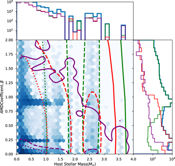
Figure 9. Distribution of AMD stability coefficient βAMD for all exoplanets at the point of their host star's ejection from the cluster as a function of the final mass of the host star. The background hexagon-binned histogram is the total for all planets and the contours represent the three planetary populations: green for Terrestrials, red for Jovians, and purple for Neptunians. Dotted lines represent the contour containing greater than 100 counts, dashed lines represent the contour containing greater than 10 counts, and solid lines represent the contour containing greater than one count.(The data used to create this figure are available.)
Download figure:
Standard image High-resolution image
5. Discussion and Closing Remarks
5.1. Discussion
The results from these simulations are revealing; they predict that a significant portion of planets within gas-ejected open clusters experience long-term stability changes due to stellar close encounters. From planetary ejections to inner-planet inspiral, it is clear that encounters fitting the parameters described in Sections 2.4 and 4.1 can drive dynamical changes in the structure of the planetary system.
As previously noted, we see that systems that become unstable always have a Neptune with a significant eccentricity change. This is expected, as when stellar systems encounter one another, the outer planets will have the largest orbital perturbation. By increasing the orbital eccentricities, these changes lower the outer planets' periapses, resulting in further orbital shifts via planet–planet interactions and, eventually, long-term instability.
We can understand the trends in our planetary systems' orbital changes through the lens of dynamical mass segregation (McMillan et al. 2007). As an open cluster evolves, stellar encounters redistribute energy throughout the cluster, attempting to drive the stars toward energy equipartition. This leads the more massive stars to move more slowly and hence sink toward the center of the cluster. As a result, more massive stars are more likely to encounter other massive stars, leading to larger encounter energies and thus greater perturbations to a planet's semimajor axis. Additionally, lower-mass stars pass through this dense core before being ejected from the cluster via evaporation, often after a single strong encounter. During such strong encounters (which our cuts highlight), even tightly packed planetary systems around these low-mass hosts can experience dramatic orbital perturbations.
Regarding the significant population of unstable Terrestrials, we note that these planets are near the critical point of β = 1 before any encounters. As such, only a small change in the angular momentum of the system is required to push this category of planet toward an instability criterion either via inspiral into its stellar host or a collision in the densely packed system. We find that while the median of our Terrestrial population remains at β = 0.945, they exceed β = 1 at the 61.63 percentile. Conversely, the Jovian and Neptunian populations only exceed β = 1 at the 99.5 percentile despite their tendency toward significant orbital change. Indeed, Dotti et al. (2019) saw similar behaviors in the stability of Terrestrials, where perturbations to the system's Jovian easily caused instability of the inner planets.
5.2. Future Work
In future papers we will improve and expand our initial conditions to better match observed clusters, such as those presented in Table 2, and implement new numerical tools to enhance Tycho's capabilities in order to make more quantitative predictions about the expected observational sample of exoplanets.
As mentioned in Section 2.1, our current methodology does not actively simulate planetary systems between stellar encounters. While this does not affect the validity of our results thanks to the robustness of the AMD stability criterion, integrating a system over long timescales will expose important nuances in its evolution. Recently, a generalized hierarchical approach to the long-term secular integration of planetary systems was described by Hamers & Portegies Zwart (2016). It was further expanded to include a secular treatment of close encounters between such hierarchical systems and is now included in AMUSE (see the SecularMultiples community code; Hamers 2018). To improve both Tycho's physical accuracy and computational efficiency, we plan to integrate this approach into our scattering experiments in the next iteration.
Additionally, Tycho does not follow planetary systems through multiple stellar encounters. Rather, it treats encounters as wholly separate from one another, regardless of a system's history or future. Most stars in these clusters only encounter one other star during the cluster lifetime and thus Tycho's approach is appropriate for the simulations presented here. However, in future larger simulations, the number of stars that undergo several encounters in their lifetime, and particularly those that migrate to the center of the cluster during the core-collapse epoch, will not be insignificant. The implementation of SecularMultiples will allow planetary systems that undergo multiple encounters to be efficiently evolved between encounters, and therefore enable proper handling of such encounter chains.
5.3. Conclusions
In this paper, we present a robust methodology, Tycho, that aims to solve the multifaceted problem of evolving planetary systems from their birth in their natal clusters to their eventual dispersion into the Galactic disk. Our proof-of-concept simulations verify that Tycho can simulate such clusters within a reasonable amount of time without compromising the physical integrity required for such work.
Examining the results of our proof-of-concept runs, we find that a significant portion (37.5%) of our remaining solar system analogs become weakly unstable due to close encounters with other stellar systems. A smaller portion become fully unstable, mainly due to the collisional criterion with the inner planet. Additionally, while systems orbiting high-mass stars experience larger changes in their semimajor axes than those around lower-mass stars, the latter experience larger dispersion in βj. Finally, 0.8% of the planets in our population were ejected from their host system and/or captured by another stellar system due to stellar close encounters.
In summary, we have developed a methodology that allows us to explore how stellar birth environments influence the evolution of planetary systems. Building upon previous numerical solutions, Tycho strikes a balance between computational efficiency of scattering experiments and direct N-body simulations. Furthermore, we plan to continue developing Tycho to enable direct comparisons between simulated and observational planetary populations, the progress of which can be followed on the project's GitHub repository (https://github.com/JPGlaser/Tycho).
This research has been supported by Drexel University's College of Arts and Science under their Doctoral Research Fellowship and their STAR program. This research made use of the NASA Exoplanet Archive, which is operated by the California Institute of Technology, under contract with the National Aeronautics and Space Administration under the Exoplanet Exploration Program. Computational resources were supported by Drexel's University Research Computing Facility through NSF Award AST-0959884. A.G. acknowledges support from NSF Astronomy and Astrophysics Postdoctoral Fellowship Award AST-1302765. The authors would also like to acknowledge Adam Dempsey (CIERA, Northwestern University) for his help in discussing the AMD stability criteria, and the AMUSE User Group.
Appendix: Summary of the Relative Angular Moment Deficit Framework
We summarize here some details of the literature on the AMD framework formalism. We assume a planetary system of Np planets orbiting a single star of mass Ms, where we may work within the heliocentric reference frame such that each planet of mass, mn has an orbit that can be described by (an, en, in, νn, ωn, Ωn) and that the total linear momentum is zero.9 Further, we assume that the normal to the reference plane is in the z direction. Thus, the vector norm of the total angular momentum is

where  . The AMD of the system, C, is defined as "the difference between the difference between the norm of the angular momentum of a coplanar and circular system with the same semimajor axis values and the norm of the angular momentum (G)" (Laskar 2000; Laskar & Petit 2017). Therefore, the relative AMD of the jth planet in the system is defined as
For each pair of planets within the system, there is a series of stability criteria which can be imposed within the AMD framework, each resulting in a specific critical AMD, Cc, where the system becomes long-term unstable if at any point for any planet  . We therefore define the AMD stability coefficient as
  , where βj > 1 results in an unstable system.
First, we consider the possibility of planetary collisions and first-order effects of MMR between planet pairs. As detailed in Laskar & Petit (2017) and Petit et al. (2017), when taking those effects into account the critical AMD can be expressed as
allowing

The piecewise nature of Cc comes from the dual stability conditions imposed (α < αR relates to collisional conditions and α ≥ αR relates to MMR conditions). It follows that there exists an αR such that Equation (A2) is continuous. We note that it makes little sense to take into account MMR effects for αR < 0.63 which corresponds to the 2:1 resonance. Using this boundary condition and evaluating the collision-based criteria of Cc with α ≈ 1 presented in Laskar & Petit (2017), αR becomes the solution to the following equation:  .
.
For α < αR, we will need to calculate the critical eccentricities which are such that the inner (m, a, e) and outer (m', a', e') planets would collide. These can be obtained from the following set of equations:
For the case when α ≥ αR, we must consider the instabilities caused by MMR overlaps. As presented in Petit et al. (2017), the square of the normalized minimal AMD to enter a resonance,  , can be written as the piecewise function, g(α, ε), defined as
where:
with Kn(x) being the modified Bessel function of the second kind. The function g(α, ε) goes to zero after α ≥ αcirc because this is the point where all orbits (including circular ones) incur MMR overlap and thus there is no configuration of stable orbits after this point.
Finally, we consider another criterion that is important for closely packed planetary systems with large mass differences: Hill stability. As presented in Petit et al. (2018), we find that the critical AMD is
This criterion is notably stricter than our previously presented Cc. As such, Hill stability may be used to quickly check if a system is AMD stable. If such a system is not Hill stable, it is still possible that it can be stabilized by the collision criterion until the point at which MMR overlap dominates (α ≥ αR) where there exist orbits that are chaotic but still satisfy the Hill stability. For visual guidance on this logic, see Figures 4 and 5 of Petit et al. (2018).
Footnotes
- 5
The Python-based interface is a community effort with its main development team based at the Leiden Observatory. It is available freely via its GitHub repository at https://github.com/amusecode/amuse.
- 6
Statistics retrieved from the NASA Exoplanet Archive on 2020 February 18 drawing from the Kepler, K2, KELT, SuperWASP, TESS, and UKIRT surveys in addition to a number of ground-based observatories and related surveys.
- 7
It should be noted that if an eccentric Galactic orbit were to be chosen for our clusters, the spatial distribution of a cluster described in Küpper et al. (2010) would be more appropriate.
- 8
We chose to vary only these parameters to demonstrate key attributes of this approach. In subsequent papers we will include initial conditions that are more directly associated with observed star clusters.
- 9
Allowing the following definitions: an is the semimajor axis, en the eccentricity, ik the inclination, νn the true anomaly, ωn the argument of periapsis, and Ωn the longitude of the ascending node.