


Abstract
Previous studies have suggested that the scattered disk is populated by planetesimals that once orbited in the reservoirs between the Jovian planets. Other studies have concluded that the source region for the Centaurs and Jupiter family comets (JFCs) is the scattered disk. Still other studies have suggested dynamical links between Centaurs and JFCs. The overarching goal of this study is to build upon our previous work and, using data mining techniques derived from big data applications, explore a database of close planet/planetesimal approaches in order to both examine these claims and demonstrate how complicated the trajectories of planetesimals wending between the Jovian planets can be—as they are subjected to impulsive alterations by close planetary encounters and resonant effects. Our results show that Centaurs, JFCs, and scattered disk objects are not dynamically distinct populations, and the paths planetesimals take over their lifetimes can be extremely complex. An understanding of this complexity offers solutions to other outstanding questions about the current solar system architecture.
Export citation and abstract BibTeX RIS
1. Introduction
The solar system metes out clues regarding its early origin and evolution grudgingly. One of the important keys to understanding the architecture of today's system lies in understanding the interactions between the Jovian planets and the primordial population of planetesimals orbiting between them. Unfortunately, the solar system has hidden or eliminated the bulk of the evidence: most members of that primitive planetesimal swarm have been accreted by planets, cast into the distant reaches of our system, or ejected into interstellar space. As a result, researchers attempting to understand the history and formation of the solar system have to piece together the clues that remain in the form of those objects that have survived this gigayears-long process of dynamical evolution.
The most numerous of these are small bodies trapped in dynamically stable reservoirs: the main-belt asteroids, the Jovian planet Trojans (de la Barre et al. 1996, Jewitt et al. 2000; Sheppard & Trujillo 2006), the Edgeworth–Kuiper Belt (EKB; Edgeworth 1949; Kuiper 1951; Fernandez 1980; Gladman et al. 2001), and the Oort cloud (Oort 1950; Morbidelli 2005; Lewis et al. 2013). Perhaps more interesting, however, are their dynamically unstable cousins: the near-Earth asteroids, Centaur objects, scattered disk objects, and short- and long-period comets (Duncan et al. 1988; Horner et al. 2003; Mumma & Charnley 2011).
Small bodies in the trans-Neptunian region are often subdivided into four broad categories: resonant objects, detached objects, scattered disk objects, and members of the "classical" EKB (e.g., Bannister et al. 2018). The classical EKB contains objects moving on stable orbits with semimajor axes between ∼40 and ∼47 au (e.g., Petit et al. 2011) and are still sometimes referred to as "cubewanos," after the first member discovered, 1992 QB1 (Jewitt & Luu 1993). This population is sometimes divided into two subpopulations: the "cold classical" and "hot classical" objects (e.g., Doressoundiram et al. 2002). The "cold classical" objects move on dynamically "cold" orbits, with low eccentricities and inclinations, while the orbits of "hot" disk objects are more excited, with greater inclinations and/or eccentricities.
Unlike the asteroid belt, where member objects reside in a dynamical abode with 4.6 billion yr of near-permanence, the orbits of many outer solar system bodies are more ephemeral. The scattered disk is a dynamically unstable counterpart to the EKB, containing objects whose orbits bring them sufficiently close to the orbit of Neptune that they exhibit dynamical instability on billion-year timescales (e.g., Lykawka & Mukai 2007a). This population has been regularly invoked as being the most likely proximate parent population for the solar system's Centaurs: dynamically unstable objects with perihelia between the orbits of Jupiter and Neptune (e.g.; Grazier et al. 1999a, 1999b; Horner et al. 2004a, 2004b).
The detached trans-Neptunian objects are those that move on orbits that take them beyond the traditional bounds of the EKB (with aphelia in excess of 50 au) while having perihelia sufficiently distant from the Sun that they are essentially decoupled from the strong gravitational influence of Neptune (e.g., Emel'yanenko et al. 2003; Brown et al. 2004). It has been speculated that these objects might be the result of perturbations from an additional, as yet unseen planet (e.g., Gomes et al. 2006; Batygin & Brown 2016; Sheppard & Trujillo 2016) or produced directly from objects in the scattered disk through a process of resonance sticking and orbital circularization (e.g., Lykawka & Mukai 2007a).
Due to the chaotic processes that drove solar system formation, it is highly likely that the scattered disk and detached trans-Neptunian populations are heavily polluted with material that formed in the interplanet reservoirs. The same is likely true for the hot classical disk, the plutinos, and the Jovian and Neptunian Trojans (e.g., Walsh et al. 2011; Seccull et al. 2018). Those objects were then cast and nudged and hurled into orbits beyond Neptune's present orbit through a combination of resonant effects and close encounters with the Jovian planets. These populations have continued to be sculpted by the planets' influence over the age of the solar system.
Observations of these small-body populations at the current epoch provide clues to the solar system's past and hints at the evolutionary pathways that brought the solar system to its current configuration, but observations alone are insufficient to fully disentangle the history of our planetary system. Numerical simulations allow researchers to create and test a wide variety of scenarios in order to progress with our understanding of solar system architecture using an assortment of different hypothetical starting conditions to advance these systems over time and assess whether the final states mirror observational truth. Such simulations have long been used to study the formation and evolution of the solar system's small-body populations, attempting to tie observed features in the distribution of those objects to the orbital evolution that must have created them. Such work has led to a wide variety of potential "pasts" for the solar system, some of which feature large-scale migration of the giant planets to their current orbits (e.g., Malhotra 1995; Tsiganis et al. 2005; Lykawka et al. 2009; Lykawka & Horner 2010; Walsh et al. 2011).
The dynamical evolution of planetesimals over time is driven by a variety of physical processes and by both gravitational and nongravitational forces. For bodies larger than ∼1 mm in diameter, although nongravitational forces such as the Yarkovsky effect (Farinella et al. 1998; Bottke et al. 2006), solar radiation pressure, and cometary outgassing (Marsden et al. 1973) can play roles in influencing their long-term evolution, the lives of these bodies are dominated by the effect of gravitational perturbations.
Resonant influences of the planets can shepherd and sculpt bodies in metastable niches like the asteroid belt and classical EKB, leading to the fine structure observed in their distributions (e.g., Chiang et al. 2003; Minton & Malhotra 2009). For bodies that experience close planetary passages, however, such encounters are chaotic in nature and can radically alter their orbital elements (e.g., Koon et al. 2001; Horner et al. 2004b; Grazier 2016, hereafter G16). Such encounters are akin to the gravity assists that spacecraft navigators use to propel probes into the inner- and outermost reaches of the solar system and play a vital role in transporting small bodies from one region of the solar system to another. Large and/or multiple encounters also ensure that, in the end, most unstable objects are removed from the system entirely, often after following highly circuitous trajectories through the solar system. The overarching goal of this study is to build upon our previous work and demonstrate how complicated the trajectories of planetesimals wending between the Jovian planets can be—as they are subjected to impulsive alterations by close planetary encounters and resonant effects—and to develop an understanding of the complexity that results and new insights into the structure of the solar system today.
In assessing the validity of simulated dynamical models, a common data analysis strategy is to output state vectors—heliocentric or barycentric positions and velocities—or orbital elements for all objects at the beginning of the simulation, synchronously, at regular intervals, as the simulation evolves, and, finally, at simulation end. In the interstices between periodic data outputs, aperiodic, or asynchronous, scenarios are playing out in the simulation's virtual realm–scenarios whose effects can be more challenging to record and analyze, sometimes due simply to the data volume or computational expenditure necessary to capture and analyze them in their entirety. The asynchronous dynamical events that occur within these interstices provide context for the synchronous information, however, and yield important insights into the architecture of the solar system of today.
G16 reported on a large series of simulations that sought to revisit the work of George Wetherill (Wetherill 1994), whose study is often cited as the basis for the concept—once widely accepted in the astronomical/astrobiological literature and still regularly discussed in popular-culture documentaries—that Jupiter defends the terrestrial planets from comets raining from the depths of the solar system. In recent years, that argument has been largely refuted, with a series of studies (Grazier et al. 2008; Horner & Jones 2008, 2009; Horner et al. 2010; G16) showing that Jupiter is at least equally likely to hurl objects onto Earth-threatening orbits as it is to protect us from that threat. Nevertheless, it is still interesting to revisit the work of Wetherill with modern computational methods to examine in more detail the fate of objects that initially move on orbits between those of the giant planets. In that light, part of the G16 study was an exploration of the evolution of 60,000 simulated massless planetesimals evolving from initial orbits located in the reservoirs between both fully formed Jovian planets and their planetary cores—what Wetherill called "failed Jupiters"—over a period of 100 Myr. One important outcome of that study was the confirmation that, today, rather than being an impenetrable shield, Jupiter is equally likely to send comets on Earth-threatening trajectories as it is to deflect them away or accrete them.
The main focus of this study is to explore possible planetesimal evolutionary paths both at the current epoch and during the late stages of planet formation—in particular, the influence of planet/planetesimal close approaches—by performing a deeper dive into the full-mass simulation output from G16 by mining a separate data set generated as part of that study but heretofore unanalyzed. This study differs in approach in that it does not solely examine the state of the simulation synchronously. Instead, the approach undertaken in this study is more similar to a "big data" trend analysis using structured asynchronous data: in particular, the impulsive changes to planetesimal orbits resulting from close planetary approaches, a novel methodology with respect to the state of the art.
We discuss this data analysis process in greater detail in a companion paper (Grazier et al. 2018, hereafter GHC18), where we present a model for the process by which Centaur objects are converted into Jupiter family comets (JFCs). Among other findings, in this study, we present the inverse model—how JFCs are converted back into Centaurs—and also explore the implications of the process of converting Centaurs to JFCs.
In the sections to follow, we first present our modeling approach, based largely upon previous work by Grazier et al. (2005a, 2005b, 2013) and G16, in Section 2. In Section 3, we explore the output of this analysis in order to identify trends and correlations in the behavior of the simulated planetesimals. Then, in Section 4, we focus on specific applications—in particular, planetesimal migration to the scattered disk and back and into JFC orbits, with implications for the outer asteroid belt (OAB), the formation of the irregular satellites, the blue and red populations of Centaurs and trans-Neptunian objects, and the origin of Ceres. We present our conclusions in Section 5. Taken as a whole, our study reveals the rich complexity of planetesimal evolution in the solar system—past, present, and future—and sheds light on several outstanding issues in solar system dynamics.
2. Method
For one component of the G16 study, the author carried out a suite of 100 Myr simulations that followed the orbital evolutions of particles from three 10,000 particle ensembles originating within the Jupiter/Saturn (JS), Saturn/Uranus (SU), and Uranus/Neptune (UN) interplanet gaps. The initial particle distributions covered a broad range of inclinations and eccentricities (and are described in more detail in G16). In all cases, however, their perihelia were exterior to the orbit of Jupiter and their aphelia interior to Neptune. As a result, the entire suite of test particles studied initially fell under the dynamical class of Centaur objects.
It is an important distinction that there is a difference between simulating 10,000 test particles originating in the gaps between the Jovian planets and simulating a protoplanetary disk. Since particles in these simulations are treated as massless and exert no influence on the planets or other particles, each 10,000 particle simulation can be viewed equivalently as a study of a lone particle with 10,000 different initial conditions. This is a useful way of viewing simulations of this nature relative to the solar system of today. Given the rate at which the Jovian planets, and even planetary cores, would have ejected planetesimals from the early solar system (e.g., Dones et al. 2015; G16), it is highly unlikely that an appreciable amount of planetesimal material remained in the reservoirs between the Jovian planets by the time they reached their final masses (Grazier et al. 1999a, 1999b, 2014, hereafter GCS14; G16). What was there will, in the main, have been significantly more excited—with higher average eccentricities and inclinations—than the initial conditions in these simulations. Consequently, despite the high number of particles in the Centaur region in these simulations relative to what is observed today, and irrespective of what evolutionary method drove the solar system to its current configuration, the dynamics reflected in these simulations is analogous to the dynamics in the late stages of planetary formation in addition to what is possible in the present day.
The numerical integration scheme employed in the simulations was a modified 13th-order Störmer multistep integrator (Störmer 1907) that both achieves and maintains the error growth limit known as Brouwer's Law (Brouwer 1937) for long-term integrations of the Sun and Jovian planets. For all simulations explored in this study, the final system energy error after 100 Myr is  (10−10) or less, while the position errors of all Jovian planets are not more than
  (Neptune) and
  (10−3) (Jupiter) rad. The details of the method and its implementation are reported in Grazier et al. (1999a, 2005a, 2005b).
In those simulations, the Sun and planets interacted gravitationally, while planetesimals were massless and influenced by only the Sun and Jovian planets, not one another. Initial planet and Sun GM values were extracted from JPL Ephemeris DE 245, and although terrestrial planets were not included in the simulation, their masses were added to that of the Sun.
The code that accommodates the varying dynamical timescales associated with planet/planetesimal close approaches—as well as collision detection—is a time-adaptive coupling of the modified Störmer integrator to a high-order interpolation scheme. Whenever the simulation software detects that a particle has entered a planet's gravitational sphere of influence (Danby 1988), it stores heliocentric state vectors for the planetesimal, as well as those for all massive objects in the simulation. Upon exit from the planet's sphere of influence, the particle state vectors are again stored, so that the encounter's effect on the planetesimal's orbital elements are easily calculated and "interesting" encounters can be reexamined readily and/or visualized in closer detail. Particles were removed from the simulations by colliding with the Sun or Jovian planets or when they were ejected from the solar system. The method is described in detail in Grazier et al. (2013).
The analysis approach taken in this study is more aligned with the big data analytics used by consumer retail stores or Hollywood studios (see GHC18) than the analyses used in previous dynamical studies. The data mining code was written in C on a single-processor machine, rather than on a multiprocessor machine and employing a dedicated data reduction language. The procedure used to extract information from the close-approach database is akin to the two-part map and reduce procedures used to analyze trends and relationships that exist within big data sets. In the first pass, information is extracted from the database and preliminarily filtered by zone of origin or even a particular simulation instance, and values of interest for each event are calculated and stored. During the second pass—what would be the reduce pass—event instances are tallied, interrelationships calculated, or correlations established.
The overall project proceeded from general to specific: the first dive into our data set was with the intent of determining basic close-encounter statistics and correlations, such as orbital element changes due to close approaches and implications of correlations in orbital element changes. The second dive was to establish all possible planetesimal evolutionary pathways that exist within the data set, and subsequent efforts were with the intent of answering specific or outstanding questions raised in the first two efforts.
3. Results
3.1. Close Approaches: Bulk Statistics and Correlations
An examination of the close approaches modeled in these simulations revealed that they mirrored the same wide variety of complex behavior seen observationally. While some particles were simply accreted by the planets or had their orbital energies boosted to ejection velocities, some became temporarily gravitationally bound to the planet they encountered, with some of these captures—known as temporary satellite captures, or TSC orbits—lasting for years, decades, and, in some instances, centuries. Some particles were even temporarily captured into orbits around a planet before impacting it much the same way comet Shoemaker–Levy 9 impacted Jupiter (e.g., Hammel et al. 1995).
We began our investigation by exploring the statistics of these encounters with an emphasis on how select orbital elements change across encounters. Tables 1–3 show the changes in semimajor axes, eccentricities, and inclinations for close encounters with each of the Jovian planets within each of the simulations. Table 1 displays the tally and percentages of encounters that lead to both increases and decreases in particle semimajor axes.
Table 1. The Percentages of All Encounters as a Function of Planet and Simulation that Result in Semimajor Axis Increases (% Out) and Decreases (% In), as Well as the Average Semimajor Axis Decrease per Encounter in au
| JS | |||||||
|---|---|---|---|---|---|---|---|
| Count a Increase | Ave Δa Inc.(au) | Count a Decrease | Ave Δa Dec. (au) | % Out | % In | Ave Δa (au) | |
| Jupiter | 163570 | 3.53 | 169994 | −2.78 | 49.1 | 50.9 | 0.32 |
| Saturn | 71221 | 5.40 | 74650 | −3.89 | 47.0 | 53.0 | 0.65 |
| Uranus | 9529 | 2.47 | 9554 | −2.32 | 50.1 | 49.9 | 0.07 |
| Neptune | 3144 | 6.73 | 3186 | −4.75 | 49.9 | 50.1 | 0.95 |
| SU | |||||||
| Jupiter | 106063 | 3.56 | 110116 | −2.84 | 49.1 | 50.9 | 0.30 |
| Saturn | 74151 | 6.13 | 83618 | −4.50 | 47.0 | 53.0 | 0.50 |
| Uranus | 31239 | 2.82 | 31149 | −2.35 | 50.1 | 49.9 | 0.24 |
| Neptune | 14178 | 8.36 | 14237 | −6.29 | 49.9 | 50.1 | 1.02 |
| UN | |||||||
| Jupiter | 58964 | 3.51 | 60990 | −2.75 | 49.2 | 50.8 | 0.33 |
| Saturn | 46747 | 6.79 | 53517 | −5.18 | 46.6 | 53.4 | 0.40 |
| Uranus | 51781 | 3.00 | 53363 | −2.55 | 49.2 | 50.8 | 0.18 |
| Neptune | 40719 | 7.86 | 41788 | −6.21 | 49.4 | 50.6 | 0.73 |
Note. With one exception (Uranus in the JS simulation), every planet has more encounters where particles acquire a net decrease in semimajor axis post-encounter, rather than an increase. When the magnitudes of the changes for the encounters are averaged, the overall trend is that particles migrate generally away from the Sun and to the outer solar system.
Download table as: ASCIITypeset image
Table 2. The Percentages of All Encounters—as a Function of Planet and Simulation—that Result in Eccentricity Increases (% Inc) and Decreases (% Dec), as Well as the Average Eccentricity Decrease per Encounter
| JS | |||||||
|---|---|---|---|---|---|---|---|
| Count e increase | Ave Δe Inc. | Count e decrease | Ave Δe Dec. | % Inc. | % Dec. | Ave Δe | |
| Jupiter | 167232 | 0.072 | 166332 | −0.071 | 50.1 | 49.9 | 0.001 |
| Saturn | 73804 | 0.042 | 72067 | −0.038 | 50.6 | 49.4 | 0.002 |
| Uranus | 9587 | 0.011 | 9496 | −0.010 | 50.2 | 49.8 | 0.000 |
| Neptune | 3199 | 0.018 | 3131 | −0.016 | 50.5 | 49.5 | 0.001 |
| SU | |||||||
| Jupiter | 108253 | 0.072 | 107926 | −0.071 | 50.1 | 49.9 | 0.001 |
| Saturn | 78628 | 0.049 | 79141 | −0.048 | 49.8 | 50.2 | 0.000 |
| Uranus | 31621 | 0.026 | 30767 | −0.022 | 50.7 | 49.3 | 0.002 |
| Neptune | 14531 | 0.038 | 13884 | −0.037 | 51.1 | 48.9 | 0.002 |
| UN | |||||||
| Jupiter | 60373 | 0.070 | 59581 | −0.069 | 50.3 | 49.7 | 0.001 |
| Saturn | 49226 | 0.048 | 51038 | −0.049 | 49.1 | 50.9 | −0.001 |
| Uranus | 54199 | 0.031 | 50945 | −0.027 | 51.5 | 48.5 | 0.003 |
| Neptune | 42468 | 0.047 | 40039 | −0.044 | 51.5 | 48.5 | 0.003 |
Note. With one exception (Saturn in the UN simulation), every planet has more encounters where particles acquire a net decrease in eccentricity—circularizing the orbit—post-encounter than an increase.
Download table as: ASCIITypeset image
Table 3. The Percentages of All Encounters—as a Function of Planet and Simulation—that Result in Inclination Increases (% Inc) and Decreases (% Dec), as Well as the Average Inclination Change (in Degrees) per Encounter
| JS | |||||||
|---|---|---|---|---|---|---|---|
| Count I Increase | Ave ΔI Inc. (deg) | Count I decrease | Ave ΔI Dec. (deg) | % Out | % In | Ave ΔI (deg) | |
| Jupiter | 166847 | 2.707 | 166717 | −2.718 | 50.0 | 50.0 | −0.005 |
| Saturn | 74704 | 1.585 | 71167 | −1.556 | 51.2 | 48.8 | 0.052 |
| Uranus | 9701 | 0.676 | 9382 | −0.636 | 50.8 | 49.2 | 0.031 |
| Neptune | 3347 | 1.285 | 2983 | −1.252 | 52.9 | 47.1 | 0.089 |
| SU | |||||||
| Jupiter | 108179 | 2.719 | 108000 | −2.716 | 50.0 | 50.0 | 0.004 |
| Saturn | 81069 | 1.706 | 76700 | −1.661 | 51.4 | 48.6 | 0.069 |
| Uranus | 31716 | 1.065 | 30672 | −1.026 | 50.8 | 49.2 | 0.037 |
| Neptune | 14517 | 1.784 | 13898 | −1.657 | 51.1 | 48.9 | 0.101 |
| UN | |||||||
| Jupiter | 59892 | 2.690 | 60062 | −2.689 | 49.9 | 50.1 | −0.004 |
| Saturn | 51393 | 1.635 | 48871 | −1.609 | 51.3 | 48.7 | 0.054 |
| Uranus | 53071 | 1.116 | 52073 | −1.104 | 50.5 | 49.5 | 0.016 |
| Neptune | 42052 | 1.936 | 40455 | −1.857 | 51.0 | 49.0 | 0.077 |
Download table as: ASCIITypeset image
In this analysis, we excluded those encounters where particles either began or ended their close approach on escape trajectories and those for which the magnitude of the change in semimajor axis (Δa) was greater than 1000 au. This was done for two primary reasons. First, this study focused more on planetesimal migration in the solar system interior to the EKB, rather than migration to and from the Oort cloud. More importantly, for particles on orbits with large semimajor axes and eccentricities, small perturbations from the Jovian planets—even those that do not register as formal close encounters in our code—can result in very large changes in particle semimajor axes. In those instances, a very small number of encounters can have a disproportionate effect on encounter statistics.
Though the total number of encounters that produce increases and decreases in particle semimajor axis are close in every case, each planet has more encounters where particles acquire a net decrease in semimajor axis post-encounter than increase, with the exception of particles approaching Uranus in the JS simulation. The average magnitude of Δa increases were larger than Δa decreases, often significantly so, and as a result, the average change in semimajor axis was positive—indicating that the overall migration of particles in these simulations was outward, toward the EKB.
Table 2 shows the counts and percentages of encounters that lead to increases and decreases in particle eccentricity. Unlike the changes in semimajor axes, the percentages of increases and decreases were similar, as were the magnitudes of the changes, yielding small overall average changes. The same can be said for changes in inclination, as shown in Table 3, which displays the tallies and percentages of encounters that lead to increases and decreases in particle inclination. In contrast to the behavior of particle semimajor axes, which trend increasingly outward, both eccentricities and inclinations perform statistical random walks.
In Figure 1, we see the duration of all particle close encounters with each planet—separated by simulation—as a function of when they occurred in the simulations. In the Jupiter and Saturn plots for the JS simulations, there are few encounters after 20 Myr into the simulations. This is due to the rapidity with which planetesimals are cast out of the JS reservoir and the fact that most particles that begin in this zone are ejected from the solar system entirely (Grazier et al. 1999a, 1999b; CGS14; G16).

Figure 1. Plots of close encounter time of ingress vs. duration for all three origin zones for Jupiter (upper left), Saturn (upper right), Uranus (lower left), and Neptune (lower right).
Download figure:
Standard image High-resolution imageThe vertical structure evident in these plots is due to neither sample aliasing nor discretization; it is a manifestation of a phenomenon encountered previously in G16, where particles undergo a rapid series of encounters with the same planet. We elaborate on this in detail in Section 4.
Figure 2 displays the relative occurrences of prograde and retrograde close approaches in 10,000 yr intervals spanning the first 5 Myr of the three sets of simulations. Close approaches to all planets shared a nearly equal occurrence of being prograde and retrograde. This was independent of the planet and source zone from which the test particle originated. Moreover, the ratio showed no time dependence and only varied significantly from 50/50 when the simulations were pared down to few or distant survivors, and encounters fell prey to small-number statistics. When the investigation is extended to 100 Myr, the numbers of prograde and retrograde encounters still remain comparable.

Figure 2. Stacked column plot displaying, for each zone, the fraction of close encounters that began with the particle in a prograde orbit vs. retrograde. The plot shows only the first 5 million yr of the simulation—where the majority of the systems' dynamical evolution occurs—but a constant across simulations is that encounters are partitioned into roughly equal numbers of prograde vs. retrograde encounters.
Download figure:
Standard image High-resolution imageWhen studying the chaotic evolution of the solar system's small bodies, many studies have made use of the Tisserand parameter as a means to distinguish between different types of objects, particularly in the context of comet-like bodies (e.g., Kresák 1980; Carusi & Valsecchi 1987; Levison & Duncan 1994; Horner et al. 2003; Emel'yanenko et al. 2005; and many others).
The Tisserand parameter is a numerical quantity calculated from the orbital parameters of a small body and a planet with which it could undergo a close encounter that, to first order, is conserved over a close encounter with that planet. For cases where the orbital eccentricity of a planet can be considered to be approximately zero (and hence be neglected), the Tisserand parameter of a given small body's orbit with respect to a particular planet is defined as
where ap and a are the semimajor axes of the planet and small body, respectively, and e and i are the eccentricity and inclination of the small body's heliocentric orbit.
The calculation of TP offers insight into the degree to which a close encounter with a given planet can modify a small body's orbit. It is also used by spacecraft navigators exploring trajectory trade studies to see what bodies may be reached due to the energy boost of a gravity assist.
If TP > 3, then close encounters between the planet and small body cannot happen—the small body is decoupled from strong perturbations by the planet, and its orbit is either wholly interior to or wholly exterior to that of the planet. Values of TP between ∼2.8 and 3.0 suggest that a close encounter between the planet and the small body has the potential to vastly alter the body's orbit, while values of TP less than ∼2.0 suggest that a given close encounter will likely only result in a small change in the body's orbit. For more detailed discussion of the impact of the Tisserand parameter on the study of small-body populations, we direct the interested reader to Horner et al. (2003) and references therein.
A core tenet of studies that use the Tisserand parameter as a means to distinguish between objects that should exhibit markedly different behaviors and/or histories is the idea that the Tisserand parameter with respect to a given planet will be conserved through the course of a single close encounter with that planet. At the same time, that encounter would be expected to modify the orbit of the small body in question, which would naturally alter the value of the Tisserand parameter of that object's orbit with each of the other giant planets. In other words, through the course of an encounter with Jupiter, the value of TJ would not change, but the values for the other Jovian planets—TS, TU, and TN—could be dramatically changed.
Given our large data set of close encounters, we decided to test the commonly held assumption that the value of TP would not change through the course of an encounter with a given planet. For each close encounter we cataloged, we calculated the value of TIN at the onset of the encounter and TOUT as the particle exited the planetary sphere of influence.
In Figure 3, we plot the results from each of our individual simulations. The top row shows the results for test particles that began their lives between the orbits of Jupiter and Saturn; the middle row shows the results for those that began between the orbits of Saturn and Uranus, and the bottom row shows the results for objects that began in the region between Uranus and Neptune. From left to right, the plots show the results for encounters with Jupiter, Saturn, Uranus, and Neptune.
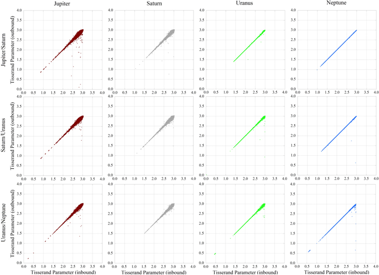
Figure 3. Tisserand parameter calculated at the close-approach entry (TIN) vs. close-approach exit (TOUT) for approaches to each planet as a function of zone of origin. One constraint was that neither the inbound nor outbound trajectory was unbound to the solar system. Events where TOUT falls far off the TIN == TOUT line are particles that ended the simulation impacting the planet that were traveling at a high heliocentric velocity at the time they were removed from the simulation.
Download figure:
Standard image High-resolution imageOn the whole, our results support the hypothesis that TP is conserved through an encounter with a given planet—with one notable exception. A tiny fraction of encounters lead to a significant reduction in the Tisserand parameter with respect to the encountered planet. Such encounters are by far the minority of cases, and a follow-on data mining pass through the output indicates that these particles were ultimately accreted by the planet and thus moving at a high heliocentric velocity when they were removed from the simulation.
3.2. Planetesimal Evolutionary Paths I
In order to explain why early observations of EKB objects seemed to reflect a blend of two populations with different eccentricity and inclination distributions, Gomes (2003) proposed a model by which outward migration of Uranus and Neptune cast some Centaur objects into the scattered disk and some into interstellar space.
Figure 4 is a recreation of Figure 1 from Morbidelli & Levison (2003), the goal of which was to illustrate the details of Gomes's model. That figure was not intended to represent an exhaustive description of all possible close-encounter scenarios or successions of encounters, but it invites the question of how such a plot might appear. Our software and database of close encounters allows us to recreate the entire evolutionary history of any particle post-simulation, including the order in which they experience close planetary encounters.

Figure 4. Recreation of Figure 1 from Morbidelli & Levison (2003), which was a graphical explanation of the Gomes (2003) model for the formation of what is now known as the scattered disk or Kuiper scattered disk.
Download figure:
Standard image High-resolution imageTable 4 shows, for all three reservoirs, two-encounter successions for the entire 100 Myr simulation. The row entries represent "From" and the column entries represent "To." Each tabulated entry, then, is the number of times an object had a close approach to the object at the left of its row followed by the object at the top of its column. For example, there were 25,344 instances when a particle underwent a close encounter with Jupiter followed by one with Saturn. By far, the most common two-encounter scenario is the progression when a particle undergoes successive encounters with the same planet. The last column represents the number of encounters where a particle exits the encounter on an escape trajectory.
Table 4. Number of Times a Planetesimal Had a Close Encounter with an Object Named in Its Row Title that Was Followed by an Encounter with the Object in Its Column Label for Different Assumptions on the Reservoir of Origin
| JS Zone | Jupiter | Saturn | Uranus | Neptune | Escape Trajectory |
|---|---|---|---|---|---|
| Jupiter | 304,649 | 25,344 | 1777 | 434 | 2943 |
| Saturn | 26,287 | 108,063 | 7755 | 2024 | 1692 |
| Uranus | 1532 | 7173 | 7868 | 2058 | 340 |
| Neptune | 319 | 1790 | 1962 | 1977 | 163 |
| SU Zone | Jupiter | Saturn | Uranus | Neptune | Ejected |
| Jupiter | 196,173 | 16,337 | 1203 | 310 | 1938 |
| Saturn | 195,30 | 124,027 | 10,280 | 2673 | 1973 |
| Uranus | 1069 | 12,442 | 38,676 | 9526 | 1059 |
| Neptune | 253 | 2589 | 8675 | 16,317 | 655 |
| UN Zone | Jupiter | Saturn | Uranus | Neptune | Ejected |
| Jupiter | 109,909 | 8774 | 637 | 157 | 1080 |
| Saturn | 10,586 | 79,766 | 7159 | 1968 | 1287 |
| Uranus | 630 | 10,751 | 72,585 | 20,500 | 1773 |
| Neptune | 155 | 2355 | 21,569 | 57,125 | 1865 |
Note. The last column represents the number of encounters where a particle exits the encounter on an escape trajectory, which is not synonymous with and is significantly less than the actual number of ejections.
Download table as: ASCIITypeset image
3.3. Planetesimal Evolutionary Paths II: Delivery to the Outer Solar System... and Back
As a follow-up to our previous studies examining the delivery of volatiles to the OAB and the terrestrial planet region (GCS14; G16), we polled the close-encounter database to explore the mechanisms that could deliver material into the inner solar system. While a small number of Uranus and Neptune encounters give particles the final gravitational kick into the inner solar system, this occurs only when the particles are on highly-eccentric orbits prior to the encounter. Only Jupiter and Saturn can deliver significant amounts of material to the OAB or deeper.
Like other studies (Gomes 2003; Horner et al. 2004a; Wood et al. 2017, 2018), our simulations show that Centaur objects migrate outward to become residents of the scattered disk. Previous studies have suggested that objects from the EKB, particularly ones on Neptune-approaching orbits, can migrate sunward to become Centaur objects. Since Horner et al. (2004a), Grazier et al. (2008), Horner & Jones (2009), and G16 showed that Centaurs originating in any interplanet reservoir can evolve into terrestrial planet–crossing orbits, it is interesting to ask: do we see evidence for planetesimals migrating first outward into the scattered disk and then inward into Earth-crossing orbits? Can we confirm that the scattered disk is a reservoir that can yield potentially hazardous objects? These hypotheses can be tested by blending synchronous state vector output with the asynchronous information in our close-approach database.
Table 5 represents our exploration of these issues. For two different values of ε (0.0 and 0.5 au), for Centaur particles starting in each interplanet reservoir, column 2 reflects the number of particles that evolve to become "fully trans-Neptunian"—defined as an object that undergoes a close planet approach where the particle has an aphelion before the encounter of less than 30 au and a perihelion post-encounter greater than (30 + ε) au.
Table 5. Fates of Particles Representing Trans-Neptunian Objects for Two Different Values of ε and Each Interplanet Reservoir
| qTNO = 30.0 ε = 0.0 au | Transitions Out | Transitions In | Max No. of Transitions | Earth Crossers |
|---|---|---|---|---|
| (1) | (2) | (3) | (4) | (5) |
| JS | 833 | 5 | 9 | 5 |
| SU | 1196 | 28 | 6 | 14 |
| UN | 1318 | 211 | 13 | 75 |
| qTNO = 30.5 ε = 0.5 au | ||||
| JS | 828 | 5 | 5 | 5 |
| SU | 1192 | 28 | 4 | 4 |
| UN | 1185 | 211 | 10 | 10 |
Note. Column 2 reflects the number of particles out of 10,000 that undergo a "transition out," defined here as a close planet approach where the particle has an aphelion before the encounter of less than 30 au and a perihelion post-encounter greater than (30 + ε) au. Column 3 is the number of particles that undergo encounters with a pre-encounter perihelion greater than 30 au and a post-encounter aphelion less than 30 au. Column 4 is the maximum number of times a particle transitions between the two groups. Column 5 represents the number of particles that have ever had a perihelion beyond (30 + ε) au and subsequently evolved to become Earth-crossing.
Download table as: ASCIITypeset image
Column 3 displays the number of trans-Neptunian particles with pre-encounter perihelia greater than 30 au that undergo close approaches with Neptune and have post-encounter orbits with aphelia less than 30 au. Column 4 is the maximum number of times a particle from each of the reservoirs transitions between being classified as a Centaur and a trans-Neptunian object.
Finally, column 5 displays the number of particles that have ever had a perihelion beyond (30 + ε) au—fully trans-Neptunian—and subsequently evolved to become Earth-crossing. While it may not be surprising, based on previous studies, that UN particles can be swept up by Neptune's sphere of influence, transported into the scattered disk, transported back, and ultimately diverted into Earth-crossing orbits, these simulations revealed that a small number of particles originating in the JS and SU zones experienced a similarly convoluted dynamical evolution.
When ε is set to 1.0 au—beyond Neptune's dynamical sphere of influence (just under 0.6 au)—we find that, although objects can evolve to become trans-Neptunian, no objects that achieve perihelion of 31.0 au or beyond returned to become Earth-crossing over the 100 Myr of our integrations.
We now explore the complex and surprising implications of the results presented in Figures 1–3 and Tables 1–5.
4. Discussion and Implications
The results of this study perform four functions. They provide useful insights into the details of the results from previous studies, including some of ours (Horner et al. 2004a, 2004b; Horner & Jones 2009; CGS14; G16; Wood et al. 2017). They corroborate results from previous studies using a vastly different numerical method: nearly all of the previous dynamical studies cited in this work were performed with symplectic or hybrid-symplectic integration schemes, as opposed to the highly accurate modified Störmer multistep integrator employed in G16. The results shed light on outstanding questions in solar system dynamics, such as the relationship between JFCs and Centaur objects and the red/blue dichotomy of Centaur, EKB, and scattered disk objects. Finally, by performing a deep dive into the G16 simulation output, we explore the intricate complexity of planetesimal trajectories both in the late stage of planetary formation and today.
The existence of the EKB (Edgeworth 1949; Kuiper 1951) was initially postulated based upon the number of observed short-period comets in low-inclination orbits. Later studies (e.g., Fernandez 1980; Duncan et al. 1988; Quinn et al. 1990) found that short-period comets could not be the result of objects captured from the long-period comet flux inbound from the Oort cloud. The long-period comets have a near-isotropic distribution (e.g., Horner & Evans 2002; Dones et al. 2004), while the short-period comets have orbits that cluster around the plane of the ecliptic. Those early studies instead suggested that the short-period comets must originate in a band of material beyond the (then) observable edge of the solar system. This prediction was soon borne out with the discovery of the first trans-Neptunian objects, starting with the archetypal EKB object 1992 QB1 (Jewitt & Luu 1993). In the two and a half decades since that discovery, our understanding of the trans-Neptunian region has blossomed, revealing a complexity far greater than we could have imagined (e.g., Bannister et al. 2018).
While the trans-Neptunian region is now considered the most likely source for the short-period comet population, dynamical studies similar to ours have speculated that, particularly in the early days of solar system evolution, planetesimals originating in the Centaur region of the solar system, through close approaches to the Jovian planets and resonant sweeping, were cast into the trans-Neptunian region, creating the population we see today (e.g., Hahn & Malhotra 1999; Levison & Morbidelli 2003; Lykawka et al. 2009). The interchange of material from orbits in the Centaur region to those in the scattered disk support this hypothesis, thus revealing that, in the present planetary configuration, it is possible for material from the Jovian planet region to become emplaced on trans-Neptunian orbits.
At the same time, the flux of material from scattered disk orbits back to the Centaur region, coupled with the fact that purely dynamical simulations are time-reversible, supports the hypothesis that the scattered disk is likely a significant source of material for the Centaur population. In summary, objects in the scattered disk originate in the Centaur region, and Centaur objects originate in the scattered disk. The two results are not mutually exclusive. One constant across all of our results is that most of the categories into which we classify small bodies in the outer solar system are equally ephemeral.
4.1. Basic Encounter Statistics and Particle Fates
Previous dynamical studies similar to G16 have disagreed in their conclusions. Some found that the net eventual particle migration is outward (e.g., Horner et al. 2004a; Wood et al. 2017, 2018). Some studies claim that the overall migration is sunward (Fernandez 1980; Duncan & Levison 1997). G16 concluded that most particles migrate to the outer solar system, but due to dynamically increased eccentricities, many pass through the inner solar system first. Indeed, the most likely story here, as seen in both Horner et al. (2004a) and G16, is that a significant collection of objects random walk in semimajor axis, journeying both inward and outward over the age of the solar system. It should be noted, too, that many comets disintegrate and decay as a result of their general friability and ongoing mass loss through outgassing (e.g., Sekanina 1984; Bockelée-Morvan et al. 2001; Sekanina & Chodas 2004, 2007), a fate that is typically not considered in dynamical studies of massless test particles.
In Table 1, we examine the statistics of particle semimajor axis changes due to close encounters with the Jovian planets. Though in all cases, the numbers are close, more particles experience close encounters that result in a decrease in semimajor axis rather than an increase, but the larger magnitudes of the positive semimajor axis changes result in an overall outward migration. This makes sense, however, since a positive impulsive Δv will increase the semimajor axis of an orbit more than a negative Δv of equal magnitude will decrease it. For example, if a body orbiting the Sun at 1 au experiences an impulsive Δv of 1000 m s−1, its semimajor axis increases by approximately 0.07 au, but an impulsive decrease of the same magnitude results in a semimajor axis decrease of only 0.06 au.
Figure 2, as well as several previous studies (cf. Holman & Wisdom 1993; Grazier et al. 1999a, 1999b), shows how rapidly the zone between Jupiter and Saturn is evacuated, and all previous studies have concluded that most of the objects between the planets are ejected from the system entirely. Consequently, it seems highly unlikely that a Jupiter and Saturn—with masses anywhere near their current values—migrating through a disk of planetesimals would leave significant material in their wake. This is even less likely if Jupiter and Saturn were closer than they are at present, and/or they passed through the same region of the solar system twice, as has been suggested in recent planetary migration models (e.g., Grand Tack; Walsh et al. 2011).
4.2. The Relationship between Centaurs and Scattered Disk Objects
In Figure 5, panel (A) displays the semimajor axes and eccentricities for all particles surviving the full 100 Myr integration time (G16), focused on the semimajor axis range of 10–103 au. Panel (B) shows the semimajor axes and inclinations of the same ensemble. There were a small number of survivors interior to 10 au, all co-orbiting with Jupiter. The simulations also yielded Saturn, Uranus, and Neptune co-orbiters, but the Saturn co-orbiters would most likely have been perturbed out of these orbits had the simulations run to 500 Myr (e.g., de la Barre et al. 1996). Populations of planetesimals remained in the SU and UN gaps. The kinetic theory developed in Grazier et al. (1999a) indicates that an integration time of 100 Myr does not allow these zones enough time to evolve fully.
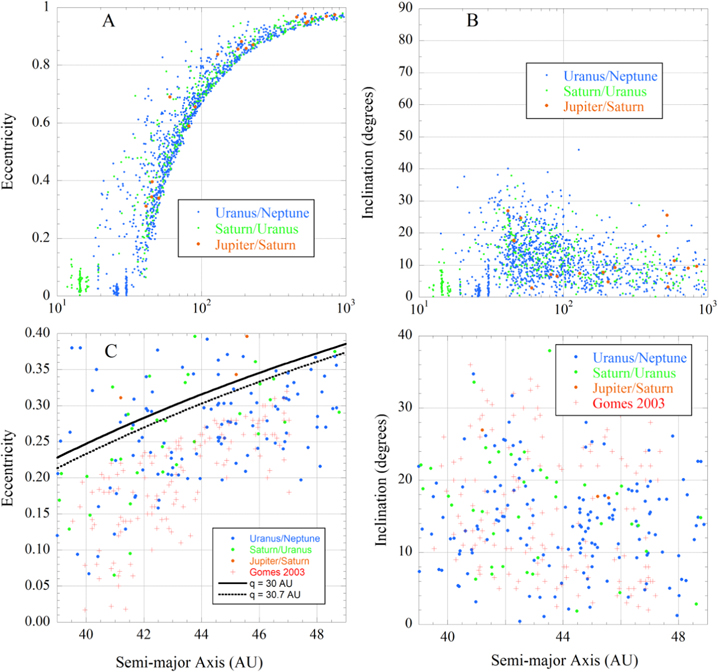
Figure 5. Plots of the semimajor axis vs. eccentricity and inclination for all particle survivors from 10 to 1000 au. Panel (A) is a subset of the particles plotted in Figure 2(b) from G16. Panel (B) displays the semimajor axis vs. the inclination for the same particle ensemble. Panels (C) and (D) plot the same information but focus (approximately) on the particles that ended the simulation between the Neptune 1:2 and 2:3 resonances at 39.4 and 47.7 au. In panel (C), the solid line corresponds to orbits whose perihelion lies at the orbit of Neptune; the dashed line represents orbits that skirt Neptune's sphere of influence.
Download figure:
Standard image High-resolution imageMany more objects that survived 100 Myr were cast still farther into the outer solar system, some to extreme distances and most on highly eccentric orbits consistent with current models of Oort cloud formation (e.g., Duncan et al. 1987; Grazier et al. 1999a, 1999b; Goldreich et al. 2004; Dones et al. 2015). Although these particles may remain bound to the solar system in a simulation, they are "practical ejectees." Once the aphelia of objects lie at distances of order 105 au or more, their orbits can be readily perturbed by the influence of the galactic tide, passing stars, and other perturbations (e.g., Biermann et al. 1983; Duncan et al. 1987). As a result, their inbound, post-aphelion orbits would be expected to differ markedly from their outbound, pre-aphelion orbits, with a typical outcome being the lifting of their perihelion distance out of the regime of the planets, decoupling them from the inner solar system. In addition to this population of "practical ejectees," many of the other particles that remained in the simulation until its termination had semimajor axes, eccentricity, and inclination distributions consistent with objects in the scattered disk.
Panels (C) and (D) of Figure 5 display the same information as panels (A) and (B) but focus narrowly on the particles that survived 100 Myr in the range between the 2:3 and 1:2 Neptune resonances. The distributions are qualitatively similar to the final states in the Gomes (2003) simulations (also displayed): re-creating a population of objects similar to those observed in the scattered disk.
Gomes's model was developed to explain the observation that the trans-Neptunian objects seemed to represent two separate populations (which we now know as the classical disk and scattered disk), and a requirement of that model is that the migration of Uranus and Neptune facilitated the implantation of objects from the then Centaur population to the scattered disk. Those implanted objects would have preferentially come from the region ranging from just interior to Uranus's orbit to just exterior to that of Neptune. The eccentricities and inclinations of the particles in panels (C) and (D) in Figure 5 are qualitatively similar to those in Gomes's work and the observed "hot" population of scattered disk objects. The most eccentric objects remaining in Gomes's study were approximately equidistant from the dashed line denoting Neptune's sphere of influence (Danby 1988). This may be another subtle indicator that distant encounters have tangible long-term influences. Such a result is not, perhaps, unexpected, as previous studies have often revealed that dynamically relevant interactions can occur for orbits that are relatively widely separated (e.g., Lykawka & Mukai 2007a).
Panel (C) contains a number of objects with higher eccentricities than in Gomes's study. This may be for a couple of reasons. This study spanned only 100 Myr, and many objects finished the simulation on either Neptune-crossing orbits or Neptune-approaching orbits that skirted the periphery of Neptune's sphere of influence. These particles—including the entirety of the JS-zone contribution to the cubewano population—would very likely have been perturbed out of these orbits had the simulation been allowed to run longer. In addition, we cannot rule out the possibility that the different numerical methods used in these two studies produce subtly different results. Nevertheless, a qualitatively similar ensemble of "hot" population objects is emergent in these simulations when neither Uranus nor Neptune migrate.
Another manner in which our results resemble those of Gomes (2003) is that the final population shows only a small number of "twotino" particles, with semimajor axes at Neptune's 1:2 resonance and plutinos at the 2:3 resonance. This could, again, be due to the fact that the present study covers only 100 Myr, or because some migration is necessary in order to make the process of resonant capture efficient (e.g., Malhotra 1995; Lykawka et al. 2009). How these objects were captured at these distances, and if they were in fact "captured" at all or randomly boosted to these orbits by close-encounter geometry—a natural outcome of a large number of particles and of close approaches—would be worthy of further study.
4.3. Close Approach–driven Migration and More on the Relationship between Centaurs, JFCs, and Scattered Disk Objects
In GHC18, the companion paper to this, we present a model for the process by which Centaur objects are converted into JFCs. In that model, once a Centaur enters a Jovian sphere of influence, the sole determinant of whether it becomes a JFC is the egress geometry. Figure 6, which is Figure 3 in GCH18, depicts a gravity-assist geometry on the left-hand side and a Centaur-to-JFC geometry on the right-hand side.
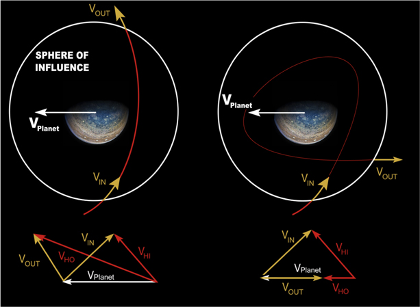
Figure 6. Two depictions of the ways in which close approaches alter planetesimal trajectories. Most encounters are of the geometry shown on the left-hand side: a single hyperbolic pass. The vector diagram beneath shows that although the magnitudes of the inbound (vin) and outbound (vout) planet/planetesimal relative velocity vectors are equal, when translated into the heliocentric frame by adding the velocity of the planet (yielding vHI and vHO), the velocity vector changes direction and increases in magnitude. This is a gravity-assist geometry—also the geometry by which JFCs are converted into Centaurs. Depicted on the right-hand side is an idealized illustration of the process by which a Centaur is converted into a JFC. In the vector diagram describing the encounter, the particle would be moving parallel to Jupiter upon exit from the close approach but much slower in the heliocentric frame, making the point where the particle leaves Jupiter's sphere of influence the particle's new aphelion.
Download figure:
Standard image High-resolution imagePrevious studies (such as Duncan & Levison 1997; Horner et al. 2004a; Horner & Jones 2009; G16) have shown that Neptune-approaching trans-Neptunian and Centaur objects can evolve to become JFCs. In order to migrate inward from more distant orbits, Table 4 suggests that this process requires many close planetary approaches, oftentimes to the same planet, in order for a planetesimal to migrate inward to Jupiter.
Levison & Duncan (1997; see also Morbidelli 2005) calculated that limits imposed by the Tisserand parameter constrained the degree to which a single close planetary approach can affect a planetesimal orbit. Both Levison & Duncan (1997) and Horner et al. (2003, 2004a) suggested that any inward migration of Centaurs was necessarily piecewise and driven by a next-neighbor hand-me-down process, with Neptune transferring a given object to Uranus's control, Uranus passing it on to Saturn, and so on.
The "close-approach network" suggested by Table 4 may initially seem to be at odds with this claim, but although Table 4 indicates that a planetesimal encounter with Neptune can immediately be followed by one with Jupiter, this does not entirely contradict those earlier works. A key point is that the Tisserand parameter is "approximately conserved" across a close approach. The earlier studies suggested that planetesimal evolution is principally driven by a series of single passes that hand a planetesimal to its neighbor, but Table 4 shows overwhelmingly that the most common sequence of consecutive close approaches is successive encounters with the same Jovian planet. So, in much the same way as the Galileo or Cassini spacecraft—both of which used multiple gravity assists with one specific planet to reach the outer solar system—our simulations reveal that planetesimals can evolve similarly, with multiple close passes by the same planet, before being "handed" to another planet, one that may not be a "next-orbit neighbor."
In our simulations, out of the 2935 UN-zone particles that eventually encounter Jupiter, only 30 particles reached Jupiter by lone encounters with Uranus and then Saturn and only one by a series of single encounters starting with Neptune. Owing to a combination of multiple passes by the same planet, resonant interactions, and distant encounters, 750 particles from the UN zone encountered Jupiter yet skipped encounters with either Uranus or Saturn. Of the particles from the UN zone that eventually encounter Jupiter, the "average" particle has one encounter with Neptune, five encounters with Uranus, and 21 encounters with Saturn before its first encounter with Jupiter.
There is an old expression that states, "An orbit always returns to the scene of the crime." Unless intercepted or scattered by another planet, a planetesimal will typically return to the point where it exited a planet's sphere of influence, and in our simulations, there were many instances where particles left Jupiter's sphere of influence on orbits having periods that were near-resonant with Jupiter's. What typically followed such encounters was a succession of close approaches with sequentially increasing or decreasing durations owing to the different depths at which the planetesimal passed through the Jovian sphere of influence. Shallow passes yield brief durations; closer planetary approaches have longer durations. These types of sequences of events give rise to the vertical structure seen in multiple panels in Figure 1.
This is, in fact, the self-same scenario that occurred more than two centuries ago, which led to the remarkably close encounter between the Earth and comet Lexell. In 1767, that comet underwent a close encounter with Jupiter, which emplaced it on a new orbit that brought it perilously close to the Earth. In 1770 July, comet Lexell passed just 0.015 au from Earth—a record close encounter between our planet and a comet. In the years that followed, comet Lexell completed two orbits in the time it took Jupiter to complete one—at which point, a second close encounter occurred (in 1779) that led to the comet being ejected from the inner solar system and potentially out to interstellar space.
Such scenarios are evident in the lower two panels of Figure 2, which display the time encounters occurred within the simulations versus their durations. The vertical structure seen in the plot for Jupiter in the upper left represents such rapid successions of encounters—with varying durations reflecting successively deeper or shallower passes through Jupiter's sphere of influence—or even TSC orbits. It is possible that, in some cases, it takes more than one pass to convert a Centaur into a JFC, and this might also be part of these series of encounters (a scenario we do not explore here, but worthy of further study). The same succession of close approaches is apparent for Saturn and the Saturn Family Comets (SFCs) in the upper right of Figure 1.
In some instances, the particle had a perihelion in the inner solar system, and successive approaches drove the particle's perihelion sunward, causing it to sequentially cross the orbits of multiple terrestrial planets. In other instances, the initial encounter placed the particle into a JFC orbit with a small perihelion distance, and subsequent encounters acted to gradually raise the perihelion. There were also instances where a rapid series of encounters suddenly stopped, there were none for a short period, and then they resumed. This occurred when successive passes occurred with increasingly distant closest points of approach and the passes "marched" out of Jupiter's sphere of influence, only to march back in from the opposite side. In G1, this effect was easier to detect in plots displaying Jovian embryo aphelion versus perihelion simply because it occurred so frequently in the simulations with full-mass planets that any structure was obscured by the sheer volume of data points.
Finally, we have also seen in the simulations that planetesimals in JFC (or Saturn family comet) orbits can undergo close approaches deep enough into the Jovian sphere of influence that the geometry is that of a gravity assist, as shown on the left-hand side of Figure 6, thus boosting the planetesimal to a more distant semimajor axis. The body may be converted into a Centaur, or the perihelion may not be distant enough for it to be Centaur, but the object is, nevertheless, no longer a JFC.
This sequence of close approaches/temporary captures has been observed on several occasions in just the past few decades in the solar system. Carusi et al. (1985) reported that several JFCs have been captured into Jupiter TSC orbits. The JFC 111-P/Helin-Roman-Crockett was captured into a Jupiter TSC orbit from 1973 December until 1985 July (Tancredi et al. 1990) and will be recaptured again in 2075. The latter encounter was used as a test case for the close-approach algorithm used in GCS14, G16, and this study (Grazier 1997; Grazier et al. 2013). We plan on an expanded exploration of the role of encounter geometry on the JFC/Centaur conversion process in a follow-up paper.
In order to assess if a link existed between photometric properties and composition, Dalle Ore et al. (2012) performed a statistical cluster analysis of the colors and albedos of trans-Neptunian objects to infer their surface composition. They found no correlation between the color and composition of objects and their semimajor axes and felt that the colors reflected the location where the bodies were formed prior to orbital evolution. Bauer et al. (2013) observed Centaurs and trans-Neptunian objects with the Wide-field Infrared Survey Explorer spacecraft and from the ground and found no significant correlation between semimajor axis, eccentricity, size, and albedo. This was taken to indicate a reshuffling of material where the source reservoir has been lost. However, Tegler et al. (2016) observed that red Centaurs display a broader distribution of colors than their blue–gray counterparts. Their orbital inclination is also narrower.
Several sets of simulations, including ours, have shown that scattered disk objects can evolve to become Centaurs, but it is likely that some objects from the classical EKB can also migrate into the Centaur region through a process of collision grinding and then slow, secular evolution. Such a process is analogous to the mechanism by which near-Earth asteroids are injected through the influence of the ν6 resonance at the inner edge of the asteroid belt (e.g., Morbidelli et al. 1994; Smallwood et al. 2018). Durda & Stern (2000) calculated that objects 4 m or larger impact comet-sized bodies every few days. Weak resonant effects acting over millions and even billions of years also contribute to the infall of objects from the trans-Neptunian region (e.g., Volk & Malhotra 2008; Lykawka et al. 2012).
Furthermore, Bauer et al. (2013) suggested that the blue–gray Centaurs are related to JFCs, consistent with their very low albedos, whereas their red counterparts may be more akin to asteroids, although the red color is more generally believed to be a signature of methanol and/or organics subject to space weathering (Strazzulla et al. 2003).
Consequently, the results of Dalle Ore, Bauer, and other spectroscopic surveys (e.g., Lacerda et al. 2014; Tegler et al. 2016) can be put into context given Figures 1 and 6 coupled with Table 4. The difficulty in determining a spectroscopic/dynamical correlation between Centaurs, objects in the scattered disk, and, to a small degree, objects in the classical EKB lies in the fact that these are not dynamically distinct populations, and their colors are not reflective of their source regions.
One possible scenario is that, because Centaurs can evolve to become JFCs and SFCs (G16; GHC18) irrespective of the interplanet reservoir of origin, and given that they can randomly walk from cometary to Centaur orbits, the dichotomy may be a reflection of surface age rather than dynamical source region (cf. Bauer et al. 2013). An object that remains distant from the Sun for extended periods, or even its entire lifetime, is exposed to cosmic rays and solar wind, which interact with methanol, organics (Strazzulla et al. 2003), or sulfur compounds (e.g., Mahjoub et al. 2017), yielding the red color. Lacerda et al. (2014) derived from albedo observations using the Herschel Space Observatory that all classical-disk objects in their data set were confined to the red group, which would be consistent with these objects being in long-term dynamically stable orbits subject to space weathering effects over the full lifetime of the solar system. On the other hand, Grundy (2009) showed, based on radiative transfer models, that a red mixture of ice and refractory organics could become darker and less red as a result of ice sublimation. This suggestion is also supported by experimental work (e.g., Poch et al. 2016). Hence, an ice- and organic-rich object plunging into the inner reaches of the terrestrial planet region is likely to outgas, yielding a younger, bluer surface. The bluer surfaces of some Centaur and scattered disk objects may simply indicate that they have been JFCs or SFCs at recent points in their dynamical lifetimes and have since migrated out of these orbits.
4.4. Delivery of Volatiles (and Ceres) to the OAB and Terrestrial Planets
GCS14 sought to compare the relative efficiencies of full-mass Jovian planets and their embryonic precursors in delivering volatile-laden planetesimals to the asteroid belt, and G16 examined the delivery of planetesimals to the terrestrial planet region. Both sets of simulations deliver hundreds to thousands of particles to the asteroid belt and terrestrial planet region over 100 Myr, most of which are delivered within the first 10 Myr and many much sooner. Those studies also showed that a less massive Jupiter and Saturn are more efficient at delivering material to these regions than they are when fully grown (Horner & Jones 2008, 2009; GCS14; G16); the full-mass planets deliver more planetesimals to the inner solar system but perturb them out of OAB- or planet-crossing orbits—or even eject them out of the solar system—much more rapidly. In much the same way that this study found that it can take multiple close approaches to a single planet in order for a planetesimal to be "handed off" to a neighbor, that study found that it may take a number of passes to a Jovian embryo in order to achieve the same effect as a lone encounter with a fully formed planet. Once perturbed into orbits that take them through the inner solar system, however, the particles in question are perturbed out of them far more slowly by embryos than the full-mass planets.
GCS14 suggested that a Ceres formed in situ could have acquired part of its volatiles, e.g., ammonia and carbon dioxide (De Sanctis et al. 2015), from the accretion of planetesimals originating in different reservoirs and across a broad range of distances. As an alternative, Ceres itself could have migrated from the outer solar system after formation beyond Jupiter's orbit. Several other large volatile-rich asteroids share similar spectral properties with Ceres (e.g., Hygiea; Vernazza et al. 2017), suggesting a common accretional environment. Many other large wet asteroids might also come from regions enriched in volatiles with respect to their current location in the main belt, but the lack of spectral characteristics of these very dark objects makes it difficult to elaborate further. It is, however, possible to envision that a large fraction of the volatiles in the asteroid belt originated in the colder regions of the solar system.
Based on these considerations, it seems plausible that Ceres could have migrated inward, had a close approach with Jupiter that placed it in a JFC orbit, with its perihelion in the OAB, then had its aphelion reduced—and moved too distant from Jupiter for the planet to cause significant influence—by collisions with extant belt material, or even as a result of dynamical friction among the potentially much more massive primordial belt.
4.5. Irregular Satellites of the Giant Planets
In addition to the "free-range" small solar system bodies discussed thus far, there is one more population of objects proposed to share a common origin with those bodies. The giant planets are accompanied by swarms of small satellites moving on highly excited, loosely bound orbits: the irregular satellites (e.g., Jewitt & Haghighipour 2007; Nesvorný et al. 2007; Holt et al. 2018). Those satellites are clustered in families that are thought to be collisional in origin and are widely accepted to have been captured by the giant planets during the latter stages of their formation, rather than having formed in situ.
When the irregular satellites are considered in terms of their spectral type, they can be broadly broken down in to two broad families: those that are red, like D-type bodies, and those that look like C-type asteroids: Phoebe, for example. The origin of the latter is debated; spectral similarities between Phoebe and C-type asteroids were originally interpreted as evidence for a migration of Phoebe from the main belt of asteroids to the outer solar system (Cuk & Burns 2004). Considering that the volatile-rich asteroids of the belt might find an origin in the region between the giant-planet orbits (Raymond & Izidoro 2017; this work), Phoebe might also have formed in that region before being kicked outward by interaction with Jupiter. On the other hand, D-type irregular satellites likely originated in the trans-Neptunian region (Nesvorný et al. 2007).
How might this evolution have proceeded? Given Table 4, Phoebe might have experienced a very convoluted series of encounters before being captured by Saturn—as may have each of the irregular satellite progenitor bodies before being captured into orbit around their current Jovian planet host. One potential scenario worthy of future study might be that red irregular satellites migrated sunward from further out into the solar system before undergoing a low-velocity capture encounter with their host planet. Figure 2 indicates that planetocentric prograde and retrograde orbits are of nearly equal probability, explaining the large population of retrograde irregular satellite orbits.
There are three possible capture scenarios.
Figure 7 shows encounter durations versus initial planet/planetesimal encounter velocity (and is a subset of the information plotted in Figure 3 of GHC18) for all encounters in the G16 full-mass simulations that did not result in ejections. All four Jovian planets capture particles into long-term TSC orbits lasting years, even decades, with Jupiter capturing more particles over a much higher velocity range than the other Jovian planets. If Saturn captured Phoebe into a loosely bound TSC orbit, which is ubiquitous in Figure 7, then a collision with an extant moon or, for a body skirting the separatrix between bound and unbound, even a passage through the rings or Saturn's upper atmosphere might dissipate enough energy to turn a TSC into a permanent satellite capture.

Figure 7. Encounter duration in days vs. planetesimal/planet relative velocity at the ingress of a close approach to Jupiter (A), Saturn (B), Uranus (C), and Neptune (D). Each plot represents encounters with a planet for particles from all three sets of simulations: JS, SU, and UN. Negative duration values represent retrograde encounters.
Download figure:
Standard image High-resolution imageAlternatively, if the planetesimal had a close approach to Saturn that placed it on a Saturn family comet orbit or a Centaur with an aphelion fixed at Saturn, subsequent approaches would occur at the particle's aphelia, and those approaches would be at low velocities. Results presented in GHC18 show that Saturn can capture objects into both TSC and SFC orbits. For a body with a perihelion at Jupiter and an aphelion at Saturn, the approach velocity is approximately 9.1 × 10⁻⁴ au day–1 if the object approached Saturn from the direction opposite to the planet's travel—a "tail chase" and the case with the most likelihood of capture. If the perihelion is near Ceres, the approach velocity is 1.8 × 10⁻³ au day–1, which, Figure 7 suggests, is too fast for Saturn to capture into a long-term encounter. An alternative to this is that Jupiter may capture a body into a JFC orbit and then, through subsequent encounters, kick the object back out to Saturn.
Depending upon the method by which the particle was handed to Saturn, it may even have approached the planet slowly during its initial encounter. Table 4 indicates that both Uranus and Neptune can pass particles directly to Saturn through an encounter or a series of encounters. If an encounter with Uranus or Neptune placed the particle's perihelion near Saturn, and the particle's initial approach to Saturn is from a tail-chase geometry, an orbit that has an aphelion near Uranus and a perihelion at Saturn's orbit would result in an approach velocity of 8.6 × 10⁻⁴ au day–1, which Figure 7 would suggest is within Saturn's ability to deflect significantly or capture. For a similar orbit with the aphelion near Neptune, the approach velocity is approximately 1.3 × 10⁻³ au day–1. Figure 7 would suggest that this initial relative velocity most likely leads to hyperbolic encounters, since a straight transit through Saturn's sphere of influence at that velocity would take over 560 days, and Figure 7 shows no encounters of that duration for that initial relative velocity.
Triton is another example of an object that is thought to have been captured from the trans-Neptunian region, making it kin to the dwarf planets currently found in the EKB (and potentially also to Ceres). The capture mechanism at Neptune may be far less complicated than that for the innermost Jovian planets, however. Indeed, long-duration encounters are to be expected for Uranus and Neptune, given the low velocities at which objects are moving in the outer solar system. In the case of Neptune, this is compounded by a quirk in the planetary masses and distances: while the radii of the gravitational spheres of influence for Jupiter, Saturn, and Uranus are similar in magnitude, at approximately one-third of an au, the radius of Neptune's sphere of influence is nearly twice this size. It is predictable that particle encounters with Neptune would necessarily be significantly longer in duration than for Jupiter, Saturn, and Uranus, thus increasing the probability of capture. Figure 7 does show that Uranus and Neptune are both capable of capturing particles into long-term encounters spanning years and even decades, implying that, along with Jupiter and Saturn, the ice giants can also capture planetesimals into TSC orbits, creating potential permanent capture opportunities.
4.6. A Cautionary Note on Close-approach Data Mining
An important outcome of this study is a cautionary one. We set out to determine what new results may be gleaned from a deep dive into the database of close approaches that are output from our simulations. That process is not without its pitfalls.
A mining of the close-approach data set reveals that 51% of JS-zone particles, 56% of SU, and 60% of UN underwent close encounters directly resulting in their ejections—but this is not synonymous with, and these numbers are significantly less than, the actual number of ejections. G16 reported that approximately 70% (70% for JS, 72% for SU, 69% for UN) of all particles are ejected in simulations with full-mass Jovian planets. This disparity grows when we account for the 1189 instances noted in G16 where particles were boosted to heliocentric escape trajectories, only to undergo a subsequent close approach causing them to be rebound to the solar system.
This implies that perturbations from distant, nonresonant encounters—those outside our definition of the sphere of influence and what constitutes a formal "close approach"—have a nontrivial influence on particle evolution. This has an observational precedent: comet Hale–Bopp passed 0.77 au from Jupiter in 1996 April as it began its long journey outward toward aphelion (Jupiter's sphere of influence is under 0.35 au). Jupiter's influence, even at that distance, was enough to alter Hale–Bopp's semimajor axis from 525 au (4200 yr period) to 370 au (2500 yr period). Grazier et al. (1999a, 1999b) showed that resonant effects and distant encounters alone can lead to planetesimal ejections when close approaches are unmodeled in the software.
In the same way that the number of formal close approaches—as registered in the software—that result in particle ejections does not recreate the number of particles actually ejected in these simulations, an examination of particles that pass through the OAB revealed that it takes care to recreate the number of particles that ever have their perihelia in the OAB from the number of particles that ever undergo encounters that inject them into the OAB—the evolutionary paths are varied and not always instantly obvious. Presumably, the results would be identical if we undertook a study of particles injected into the inner asteroid belt (IAB) or terrestrial planet region.
Figure 8 is a plot of the number of close planetary approaches that result in a particle with its perihelion in the OAB versus the number of particles that actually ever pass through that part of the belt for the JS, SU, and UN zones. After 5 Myr in the JS simulation, 5379 particles had made at least one pass through the OAB, but when close encounters were scrutinized, there were 6000 encounters that left a particle with a perihelion in the OAB. Of the 6000 encounters, 5876 were with Jupiter, 891 with Saturn, eight with Uranus, and zero with Neptune—equaling 6775 encounters, a value higher still. Subtracting 768 from this value for particles that arrived in the OAB due to encounters with both Jupiter and Saturn (implying that the particle had to migrate into the OAB, out, then back in owing to an encounter with a different planet than for the first instance) and seven due to Uranus that also experienced multiple forays into the OAB, adding the one that encountered only Uranus arrives at 6000.
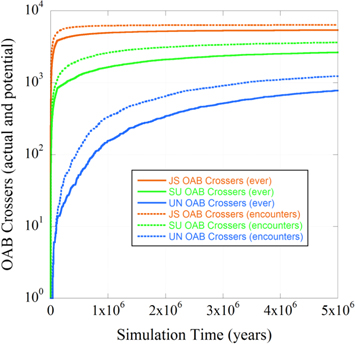
Figure 8. Number of planetesimals that undergo planetary close approaches resulting in a perihelion in the OAB compared to the number that actually ever reach the belt.
Download figure:
Standard image High-resolution imageThat particles migrate both into and out of the OAB explains why 5876 + 891 + 8 = 6000 in context, but this still falls short of explaining why more particles undergo encounters that should put them into the OAB than actually arrive there. The key to the disparity lies in encounter geometry. Of the 5876 Jupiter encounters that rendered particles OAB-bound, 4653 occurred when the particle was inbound to the Sun (defined by heliocentric r · v < 0), and 4665 were outbound (r · v > 0). Of these, 3442 arrived in the OAB through both inbound and outbound encounters, again with the constraint that the particle had to leave the belt before a subsequent encounter registered in any of the counts. Of the 891 Saturn encounters that inject particles into the OAB, 498 were inbound encounters and 492 were outbound (99 were injected both ways).
For outbound Jupiter encounters and inbound/outbound Saturn and Uranus encounters, there were hundreds of instances when an OAB-bound particle was "intercepted" by another Jovian planet. There is no disparity: a simple comparison of OAB passages versus projected passages paints an incomplete picture.
An examination of the mechanism by which close approaches caused planetesimals to pass through the OAB revealed that 5480 particles encountered Jupiter and had their perihelia lowered such that the particle passed between 2.5 and 3.3 au at perihelion. Another 3606 particles were injected deeper into the IAB, or even the terrestrial planet region, and a subsequent encounter with Jupiter raised the particle's perihelion to reside within the OAB. The intersection of these two sets—particles that were injected by both scenarios—is 3194 particles.
We found numerous examples where a simple analysis of close approaches did not yield a complete picture and should be analyzed with caution. This reveals that although our examination of close-approach data lends valuable insight into the dynamics that played out asynchronously in these simulations, a study based upon this output alone—without the supporting context of synchronous information—must be undertaken with care.
4.7. The Final Picture
In Section 3.2, we examined how a plot of all possible encounter successions from planet to planet would appear. How might planetesimals wend their way through the solar system? Table 4 indicates what possible close-approach interactions are possible, as well as which planets can eject objects into interstellar space. G16 showed that Jupiter and Saturn can convert Centaurs to inner solar system–crossing JFCs and "Saturn family" comets, and GHC18 showed how. In Section 4.4, we saw how Centaurs can migrate into the scattered disk and back. Figure 9 shows the fabulous complexity of possible planetesimal pathways constructed from these building blocks.

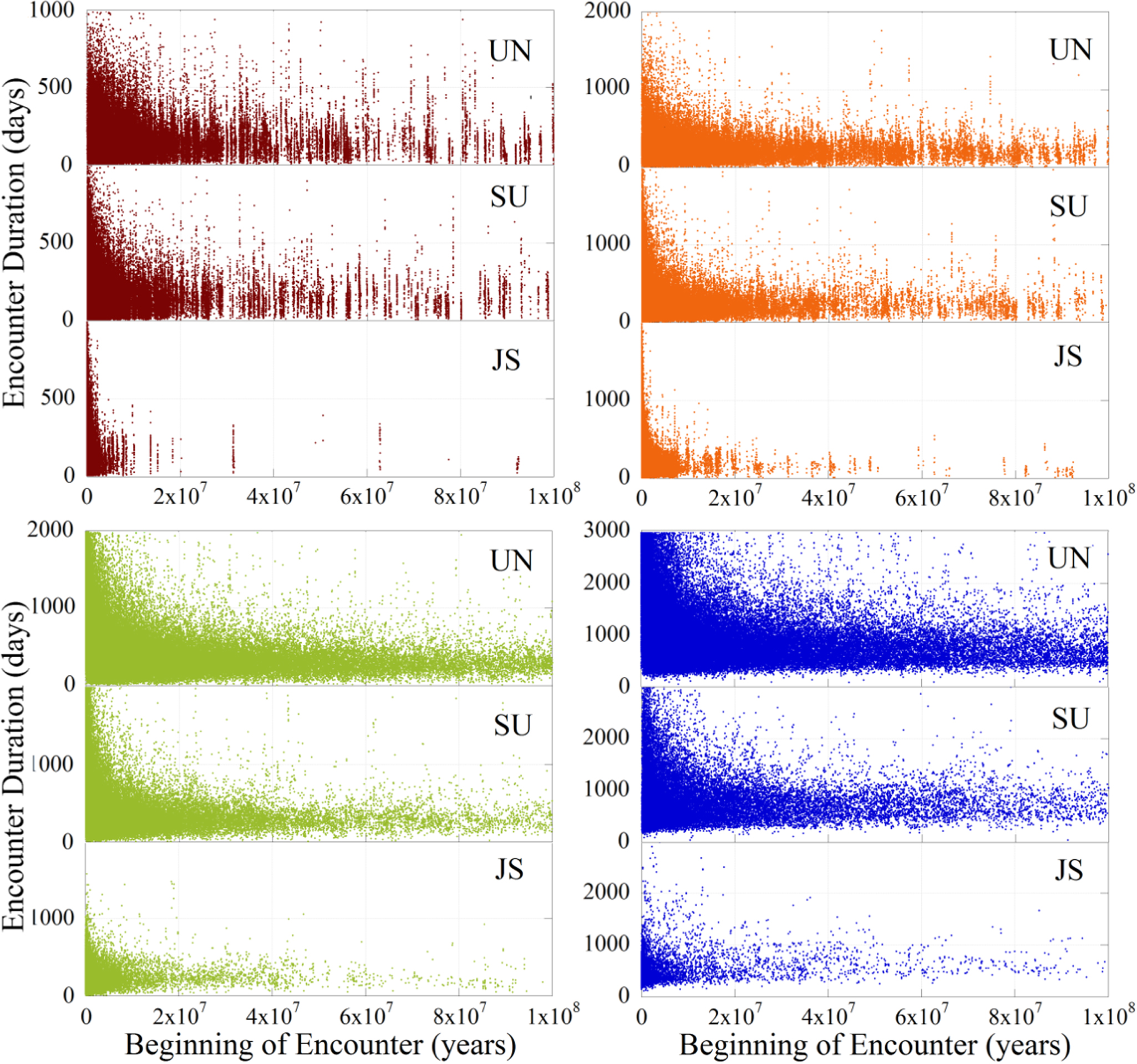
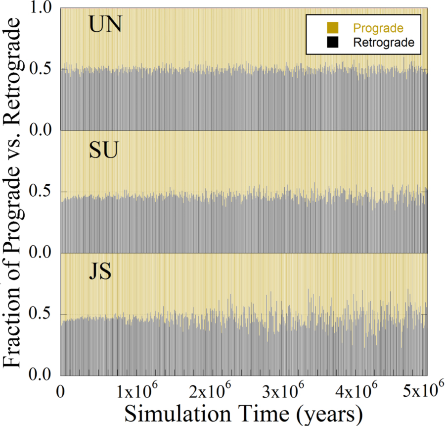
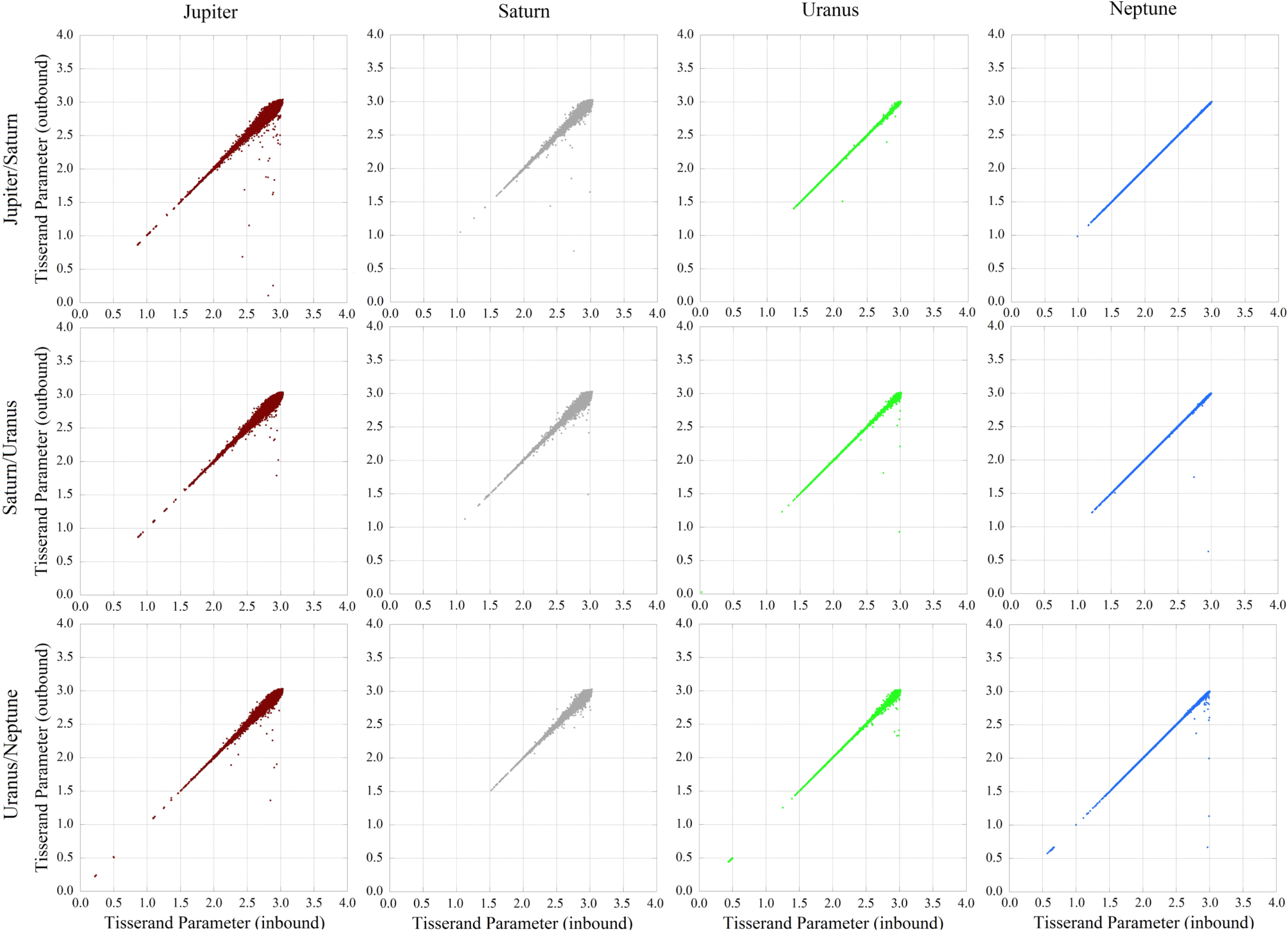
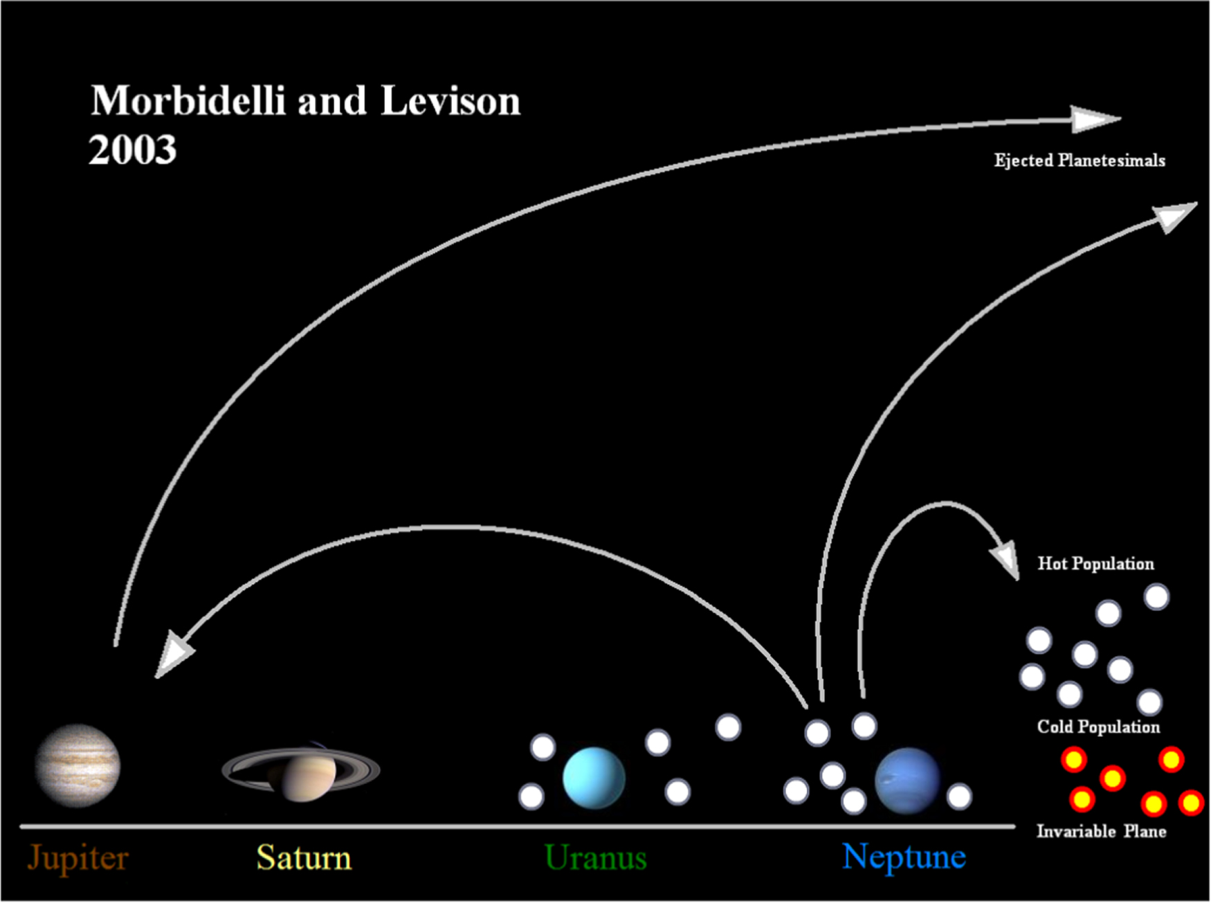
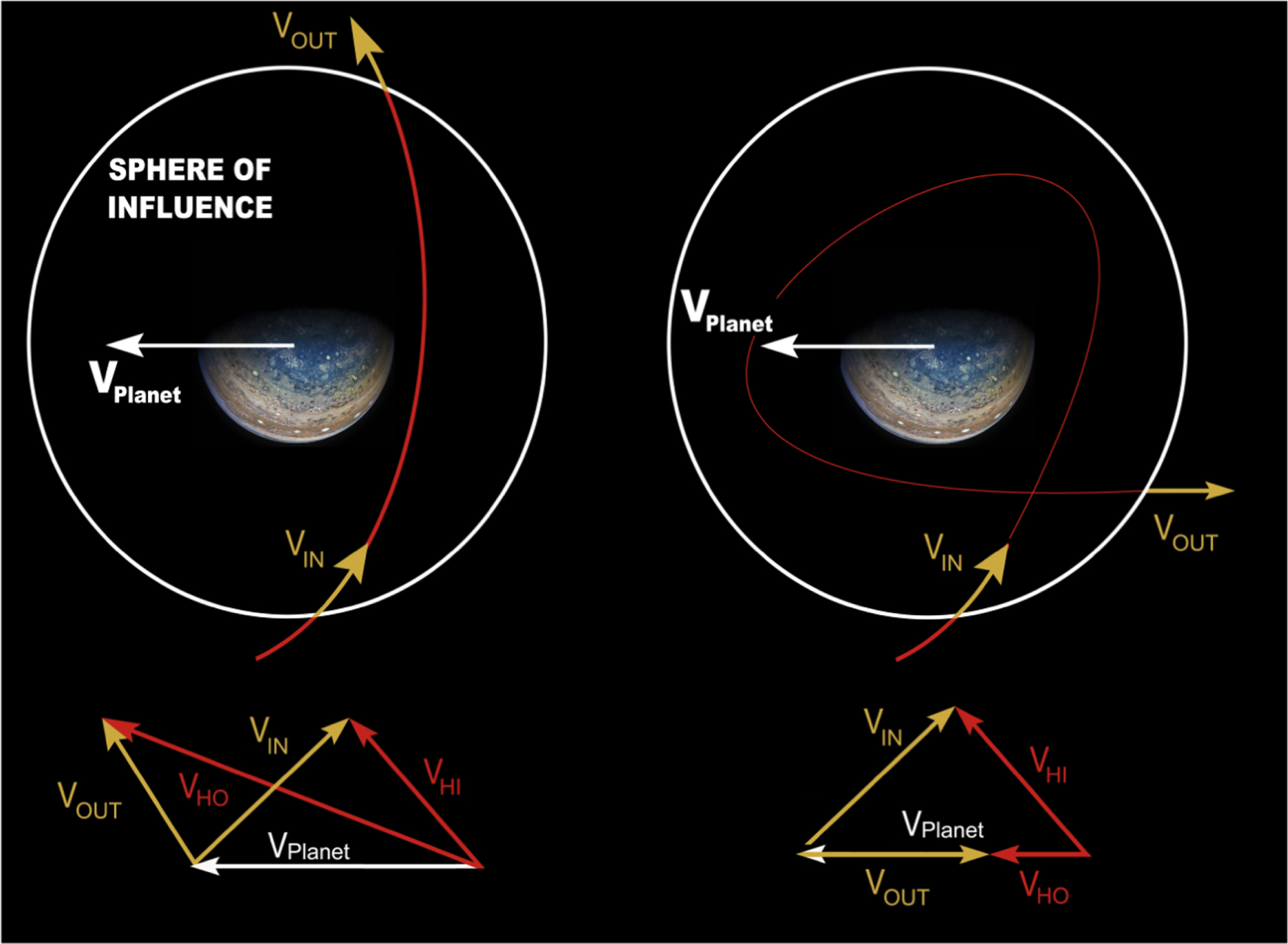
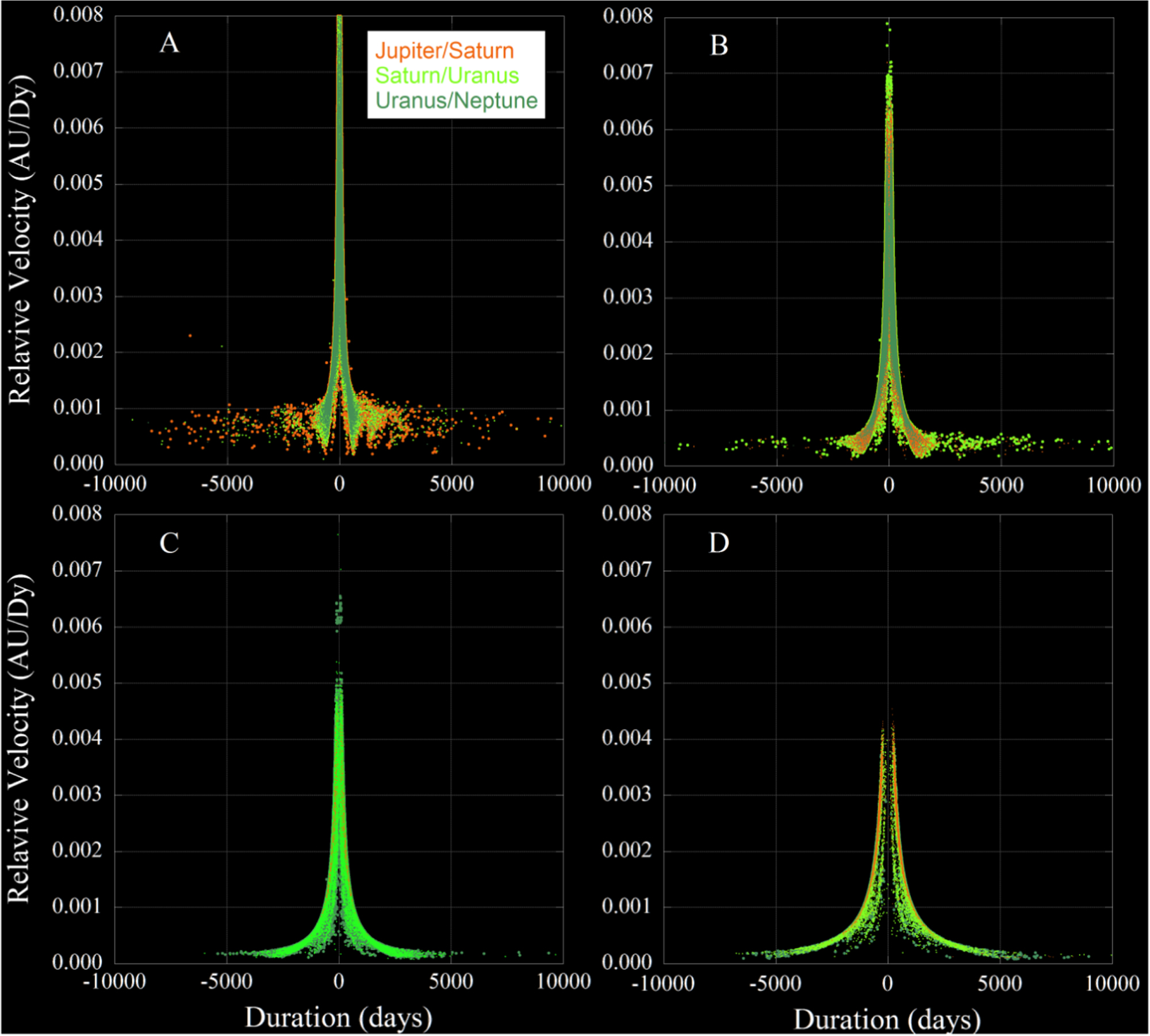
Figure 9. Graphic distillation of Tables 1 and 4, as well as results from G16 and GHC18, indicating every configuration of close-approach/ejection succession that occurred within the 100 Myr simulation. Jupiter and Saturn, and to a much lesser degree Uranus and Neptune, are able to hand material to the OAB and terrestrial planet region.
Download figure:
Standard image High-resolution image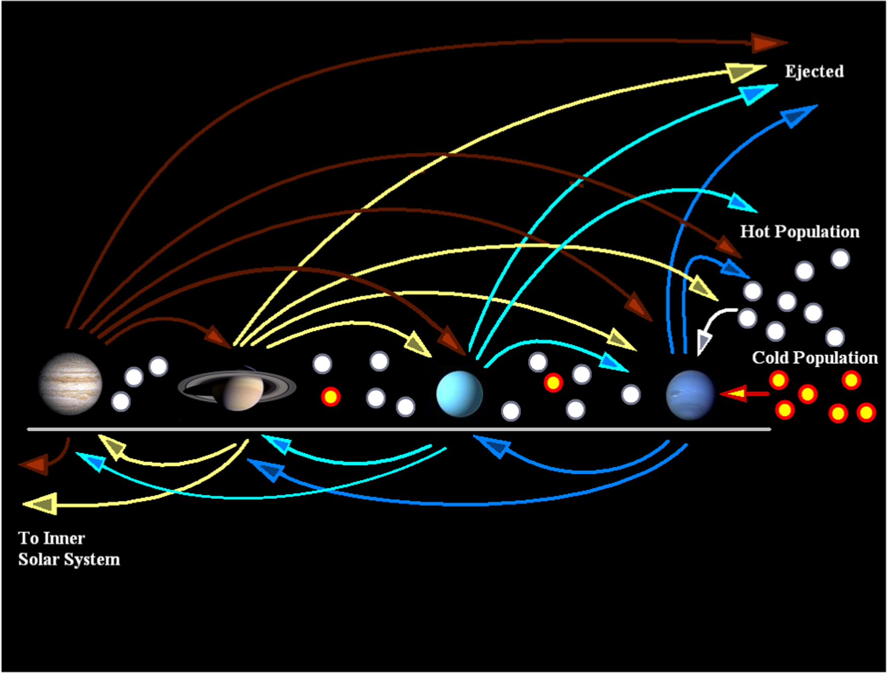
While Figure 9 opens up numerous possibilities for explaining the architecture of our solar system—like the notion that the blue/red dichotomy of solar system bodies reflects a body's history, not its dynamical source region—it simultaneously adds complications. Present taxonomic classifications are now murky. Is a mission to explore an object in the EKB really a mission to explore a very distant Centaur? Horner et al. (2004a) observed that outer solar system small bodies put into any classification scheme will change classes repeatedly over their dynamical lifetimes, often revisiting bins multiple times. Not only did this study find ample support for this, we now have a good indication of how an object changes its dynamical taxonomy: by repeated encounters with Jovian planets, often repeated encounters with a single Jovian planet—or by being captured into a JFC-type orbit.
5. Conclusions
Using a simulation output analysis approach derived from big data analytics, we have demonstrated the degree to which planetesimal evolution in the presence of Jovian planets can follow highly convoluted paths. In particular, Centaurs do not reside on orbits that remain stable over long time periods. Throughout the course of their dynamical evolution, some will be injected into the Oort cloud and scattered disk and some into the inner solar system, while most will be ejected from the system entirely. As part of this process of "planetary pinball," some scattered disk objects become Centaurs en route to the inner solar system and then to interstellar oblivion. We find that the G16 full-mass simulation, which did not employ planetary migration, produced a population of scattered disk objects similar to simulations that did employ migration. This suggests that planetary growth dominates the fate of planetesimals formed within the orbits of giant planets.
Our results show that planetesimals can follow extremely circuitous paths over time, and this may assist in resolving several outstanding solar system questions. (1) Scattered disk objects, Centaurs, and JS family comets are not dynamically distinct populations, and planetesimals can transition between these classifications many times over their dynamical lifetimes. (2) Ceres may have originated much farther out in the solar system, and it, too, may have been routed into an OAB-crossing JFC orbit before that orbit was made less eccentric, perhaps by a collision pulling its aphelion away from Jupiter. (3) The blue/red dichotomy of outer solar system planetesimals may have little to do with the dynamical source region but may reflect that blue objects were, at some point, JFCs. (4) Several processes allow planetesimals to approach the Jovian planets slowly, allowing them to be captured into irregular satellite-like orbits.
Overall, our results serve as a reminder of the glorious complexity that bedevils our study of the formation and evolution of the solar system. As ever more objects are discovered by the next generation of survey instruments, our understanding of that complexity is bound to grow still further. But through the analysis of that big data, we will eventually be able to use that complexity to disentangle the narrative of the solar system's past.
The authors thank Philip Sharp for allowing some of the simulations presented in this study to run on the University of Auckland Math Department computer network. A portion of this work was conducted at the U.S. Military Academy, West Point, NY, and part at the Jet Propulsion Laboratory, California Institute of Technology, under contract to NASA. U.S. Government sponsorship is acknowledged. The views expressed in this article are those of the authors and do not reflect the official policy or position of the Department of the Army, the Department of Defense, the National Aeronautics and Space Administration, the California Institute of Technology, or the U.S. Government.