


Abstract
We use NEOWISE data from the four-band and three-band cryogenic phases of the Wide-field Infrared Survey Explorer mission to constrain size distributions of the comet populations and debias measurements of the short- and long-period comet (LPC) populations. We find that the fit to the debiased LPC population yields a cumulative size−frequency distribution (SFD) power-law slope (β) of −1.0 ± 0.1, while the debiased Jupiter-family comet (JFC) SFD has a steeper slope with β = −2.3 ± 0.2. The JFCs in our debiased sample yielded a mean nucleus size of 1.3 km in diameter, while the LPCs' mean size is roughly twice as large, 2.1 km, yielding mean size ratios ( ) that differ by a factor of 1.6. Over the course of the 8 months of the survey, our results indicate that the number of LPCs passing within 1.5 au are a factor of several higher than previous estimates, while JFCs are within the previous range of estimates of a few thousand down to sizes near 1.3 km in diameter. Finally, we also observe evidence for structure in the orbital distribution of LPCs, with an overdensity of comets clustered near 110° inclination and perihelion near 2.9 au that is not attributable to observational bias.
Export citation and abstract BibTeX RIS
1. Introduction
Comets are the most accessible primordial bodies in our solar system, providing measurable constraints on the formation environments within the protoplanetary disk and subsequent volatile evolution that has taken place. Maintained in deep storage over much of their existence (see Dones et al. 2015), these bodies have retained a larger fraction of their volatiles as compared with other small bodies (Mumma & Charnley 2011; Ootsubo et al. 2012), such as the main-belt asteroids, which have absorbed a significantly larger solar flux over the past 4.5 Gyr. That comets hold on to their volatiles, at least in proximity to their surfaces, is what makes these bodies peculiar as the presence of ices leads to the sublimation and active mass loss as they approach the Sun that drives material from the comet nucleus surface, which in turn creates the comet's coma, tail, and trail structures.
The basic dynamical classes of comets and their implications for cometary reservoirs have been investigated for over half a century (see Oort 1950; Kuiper 1951). Although the orbital properties of comets have long been studied, efforts to constrain the most basic physical properties of the comets are more recent (see Meech et al. 2004). Statistically meaningful samplings of quantities such as volatile and dust production rates have been accumulated for several decades (e.g., A'Hearn et al. 1995; Cochran et al. 2012). However, the size distributions of comets have only recently been explored. These studies are greatly aided by the operation of space-based visual-band observatories, such as the Hubble Space Telescope (Lamy et al. 2004), and thermal-infrared observatories, such as the Spitzer Space Telescope (SST; Lisse et al. 2005, 2009; Kelley et al. 2006; Woodward et al. 2007; Bauer et al. 2008; Reach et al. 2009; Fernández et al. 2013) and the Infrared Space Observatory (Lisse et al. 1998, 2004). The bulk of these targeted observations focused on short-period comet (SPC) populations, in particular the Jupiter-family comets (JFCs). These observations are targeted at objects discovered by a variety of ground-based optical surveys, and thus they reflect the surveys' selection effects.
Observational biases can be better constrained with data from all-sky surveys that detect small bodies over a regular search pattern regardless of dynamical class. The process of accounting for observational biases when extrapolating an observed sample to an entire population is known as debiasing. Francis (2005) undertook an effort to debias observations of the underlying long-period comet (LPC) population from the comets observed by the Lincoln Labs Imaging Near Earth Asteroid Reconnaissance survey (LINEAR). This work found that only a few bodies per year larger than 2 km in diameter from the LPC population come within 1 au of the Sun. The consequential impact rate for Earth for such a population would be on the order of one every few hundred million years. Interpreting the underlying measurements required several assumptions to be made, including the fractional area of the surface that is active, the evolution of cometary behavior over time, and the size distribution. Also, ground-based surveys like LINEAR are subject to weather and seeing variations (and thus changes in sensitivity), which complicate efforts to properly account for their detection and discovery biases.
On 2009 December 14, the Wide-field Infrared Survey Explorer (WISE) mission was launched to survey the sky simultaneously in four infrared bands, at 3.4, 4.6, 12, and 22 μm, referred to as W1, W2, W3, and W4, respectively (Wright et al. 2010; Cutri et al. 2012). NEOWISE was the NASA Planetary Science Division-funded component of the mission tasked with observing and reporting to the Minor Planet Center those comets and asteroids detected by the WISE mission with its moving object pipeline subsystem (Mainzer et al. 2011a). The survey began on 2010 January 14 observing with all four bands. On 2010 August 6 the solid hydrogen cryogen in the outer tank was exhausted and the telescope became too warm for the W4 detector to operate. The W3 band continued to provide useful data until 2010 September 29, when the cryogen in the inner reservoir was exhausted. The NEOWISE post-cryogenic phase of the prime mission began at this point using the two short wavelengths until 2011 February 1, when the spacecraft was placed in hibernation. The spacecraft was reactivated as NEOWISE, with survey observations resuming on 2013 December 13 (Mainzer et al. 2014; Cutri et al. 2015).
The observations discussed here concern the prime mission's cryogenic observations in 2010, with a particular focus on the W3 and W4 data. Wright et al. (2010) present details of the survey sensitivities in each band, as well as methodologies for extracting magnitudes and observed fluxes from the publicly available source and image catalogs (http://irsa.ipac.caltech.edu/Missions/wise.html). Salient features of the survey regarding solar system observations have been discussed in detail by Mainzer et al. (2011a, 2011b, 2011c, 2012), Grav et al. (2011b, 2012a, 2012b), Masiero et al. (2011, 2012), and Cutri et al. (2012), with particular focus on cometary and related outer solar system bodies by Bauer et al. (2011, 2012a, 2012b, 2013, 2015).
To summarize, the survey acquired images of the sky at 11 s intervals near a solar elongation of 90°, as the spacecraft traveled on a Sun-synchronous polar orbit. The scans precessed approximately 1° in ecliptic longitude each day, though the survey pattern included variations for Moon avoidance and to minimize the impact of spacecraft passages through the South Atlantic Anomaly. The exposures were 7.7 s long integrations in W1 and W2, and 8.8 s in W3 and W4, with a 47 × 47 field of view (FOV). Coverage of regions of sky varied depending on the ecliptic latitude, with a minimum of eight exposures near the ecliptic for each pass and up to several hundred exposures near the poles, but on average there were 10–12 exposures of moving objects at a particular epoch. For the purposes of clarity, we call these sets of exposures of a small body in the same region of sky "visits" (see Bauer et al. 2015).
In this work, we present an analysis of the cometary nuclei detected by WISE during its four-band cryogenic phase. The vast majority of the comets were showing extended emission from a dust coma, so we discuss our nucleus extraction method that yielded flux densities of the nuclei alone. We provide nucleus size estimates for both LPCs and SPCs from these flux measurements. We compute the observed size distributions of comet nuclei for each major dynamical class (LPCs and JFCs). Finally, we use the observed size–frequency distributions (SFDs) and observations of JFC and LPC activity from Bauer et al. (2015), and Kramer (2014) to debias these observations and provide constraints on the underlying populations following the methodology of Mainzer et al. (2011c) and Grav et al. (2012a, 2012b).
2. Observations, Photometry, and Coma Subtraction
NEOWISE/WISE detected 164 recognized cometary bodies during the four-band mission, including 56 LPCs and 108 SPCs. A total of 71 of these were detected by creating stacked images in the co-moving reference frames of previously known comets that were undetectable in the individual frames. Objects recovered from stacked images will be affected by different detection biases (e.g., they were found at different sensitivity levels) than those detected by the WISE Moving Object Processing System (WMOPS) and so are excluded from the debiasing analyses. A total of 95 of the 108 SPCs were JFCs, the remainder being 7 active main-belt asteroids, 4 active centaurs, and 2 Halley-type comets.
Several comets have been discussed in previous publications. Bauer et al. (2011) provided in-depth analysis of 103P/Hartley 2, including CO and CO2 production rates, as well as nucleus size estimates and characteristics of the comet's dust coma, tail, and trail. Bauer et al. (2012b) discussed the main-belt comets detected by NEOWISE, and Bauer et al. (2012a) reported the WISE cryogenic observations of 67P, also providing a nucleus size, CO+CO2 production constraints, and dust tail analysis that were confirmed by observations made by the Rosetta mission (see Rotundi et al. 2015). Bauer et al. (2015) discussed the W1 and W2 detections in detail, with particular emphasis on the CO+CO2 production measurements provided by observations of 39 comets, as well as the nucleus sizes extracted for the 20 cometary discoveries made during the four-band cryogenic phase of the mission. Kramer (2014) presented preliminary analyses of the dust tail in the two longest wavelength bands. Bauer et al. (2013) included Centaur comets observed by WISE as well, including C/2011 KP36 (Spacewatch), 95P/Chiron, and 174P/Echeclus.
In the course of analysis, we found a concentration of observed comets in orbital-parameter space ranging near 110° ± 20° inclination and perihelion distances between 2.5 and 3.25 au (Figure 1). To test the validity of the apparent cluster, we ran 10,000 Monte Carlo instances of a random 2D uniform distribution in inclination (0–180) and perihelion (0–6 au) and found a 99.98% significance that this clustering was not appearing by random chance. The comets in this cluster tend to have higher eccentricities as well, in excess of 0.99. However, one of the eight comets within the cluster has an orbital eccentricity <0.99. If we only consider the seven other comets, we obtain a 99.77% significance. In either case, the clustering has a >3σ significance. Several causes have been suggested for potential anisotropies in LPC orbital distributions. Dybczynski (2002), for example, examined the possibility of a single stellar passage and speculated an approximate rate of seven comets per year from such an approach, with a directional clustering and a duration of the related cometary influx on million-year timescales. Matese et al. (1999) studied the anisotropies that a planetary body in the Oort cloud region may introduce. Their work speculated on planets that were on the order of a few Jupiter masses, and such planets would likely have been detected by the WISE cryogenic mission (see Wright et al. 2014). However, recent work by Batygin & Brown (2016) indicates that planetary perturbers may fall within a smaller mass range. We speculate here that the cluster may instead be caused by a particular breakup of an object. This is the first such cluster associated among the non-sungrazing LPCs. Given that this suggested breakup would have occurred at larger heliocentric distances than the breakup of the Sun-grazer parent, the larger spread in orbital parameters is expected, as orbital modifications due to activity will have a larger effect.
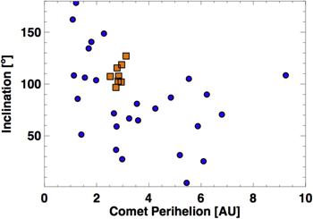
Figure 1. Cluster of LPCs in inclination and perihelion found in the NEOWISE four-band mission data. The cluster of eight comets is shown by the orange squares, and the remaining comets outside the cluster are shown in blue. Monte Carlo simulations of uniform distribution indicate a >3σ significance to the cluster.
Download figure:
Standard image High-resolution imageNEOWISE observations of those comets not discussed in previous publications and their extracted fluxes from the stacked images are summarized in Table 1. See Bauer et al. (2015) for a description of the stacking, image selection technique, and the extraction of the photometry from the images. Note that as in Bauer et al. (2015), the derived fluxes in W3 and W4 were corrected for color as prescribed in Wright et al. (2010). Stacking may produce significant signal in one or more bands depending on several factors, including the comet's activity, distance at the time of observation, and the density of background (confusion) sources in a particular band. W1 and W2 have higher confusion noise because of the higher surface density of background objects, and so they do not yield significant signal very often. Furthermore, many of the comets are detected at large heliocentric distances so that they have weak or no thermal signal in W1 or W2, while showing strong signal at W3 and W4, or only in W4 for the farthest heliocentric detections. For this reason we concentrate only on W3 and W4 detections here.
Table 1. Comet Observations
| Comet | Rhelio (au) | Delta (au) | W3 Flux (mJy) | W3_ferr | W4 Flux (mJy) | W4_ferr | Apparent Activity? (Y/N/U)a | Mid-Exposure (MJD) | Number of Frames |
|---|---|---|---|---|---|---|---|---|---|
| 7P | 4.14 | 3.94 | 0.73 | 0.14 | 11.5 | 2.4 | U | 55218.76716 | 15 |
| 14P | 3.39 | 3.16 | 2.73 | 0.51 | 14.6 | 2.94 | N | 55235.83697 | 16 |
| 17P | 5.13 | 4.93 | 0.66 | 0.13 | 8.69 | 1.86 | Y | 55330.84578 | 11 |
Note.
aY indicates apparent activity in the image (dust coma or tail), N indicates no apparent sign of activity, and U indicates the presence of coma could not be ruled out. The first column lists the comet designations. The heliocentric distance (Rhelio) and comet–spacecraft distance (Delta) are also shown in units of au. W3 and W4 fluxes (W3 flux and W4 flux) and associated uncertainties (W3_ferr, W4_Ferr) provided are from 11 aperture in units of millijanskys (mJy). Conversion from DNs to flux was carried out as described in Wright et al. (2010). The presence of coma is indicated in the eighth column ("Coma?"; Y = yes there's obvious coma, N = no obvious coma, and U = coma presence is uncertain). Values of "nan" indicate extracted flux values with no detectable signal. The midtime of the stacked image (Mid_Date) in units of Modified Julian Date (MJD) and the number of frames (Nf) co-added in the stacked image of each comet are in the last two columns.
Only a portion of this table is shown here to demonstrate its form and content. A machine-readable version of the full table is available.
Download table as: DataTypeset image
The coma subtraction methodology is the same as described in Bauer et al. (2011, 2012a, 2015) and in Fernández et al. (2013), and it was initially developed by Lamy & Toth (1995) and further modified by Lisse et al. (1999). The wings of the coma are fit along summed 3° wedges of azimuth around the location of peak brightness with a (1/r)n profile, where 0.65 < n < 1.85, in combination with a point-spread function (PSF) at the center. The W3 and W4 PSF shapes were drawn from the profiles produced by the WISE Science Data System and accessible online (Cutri et al. 2012); these are the only two bands where nucleus sizes were fit. The optimum selection of the radial extent for fitting the coma wings relative to the nucleus depends on the individual comet image characteristics, including the noisiness of the background. If the radial extent chosen is too small, the coma subtraction starts to eliminate the outer portion of the PSF, impacting nucleus size determination. If the radial extent is too large, then background noise will dominate the fit. If there is too little signal, over too small a margin, the subtraction will be dominated by noise as well, artificially increasing the measured extent of the coma.
We used four sets of wing-fitting model parameters (Table 2) in each band and selected from a subset of the model outputs. The coma subtraction removed more or less of the total signal (i.e., were "more aggressive" or "less aggressive") depending on how far out in the wings and how far in to the central condensation the coma was fit. The subset of model parameters used in each diameter fit is listed in Table 3 (complete version available online). Figure 2 shows three demonstrative examples of the stacked images of comets, along with the resulting coma-subtracted W3 and W4 images used in the derivation of nucleus diameters. We also include one example of a comet where the technique fails; this happened for only 6% of our sample and thus should not significantly affect our results. The standard deviation of the extracted nucleus magnitudes from the coma-subtracted images for the subset of models applied is folded into the photometry uncertainty.
3. Analysis
3.1. Diameters and Beaming Parameters
Table 3 gives the derived diameters for the comet nuclei. The analysis was carried out using 11 apertures except in a few cases, where 9 or 22 apertures were used (as noted in the table) to avoid image artifacts or sample more extended coma signal. Note that the value derived from aperture photometry of a comet at infrared wavelengths, the product of average grain emissivity, ε, the fractional area filled by the coma, f, and the projected size of the aperture radius at the distance of the comet, ρ, i.e., εfρ, is a proxy for the quantity of dust produced by the comet and was computed directly from the 11 aperture signal (see Table 3 for W3 and W4), and analogous to the value of Afρ more commonly used for visual wavelength observations (see A'Hearn et al. 1984). For comets observed in the infrared, the average grain emissivity ε is substituted for albedo in the value εfρ (Lisse et al. 1998; Kelley et al. 2013); the values are expressed here in units of log cm. Many comets did not have any significant W1 signal, typically because the confusion noise was higher at 3.4 μm than at 12 and 22 μm. After subtracting out the flux contributions from the nucleus in W3 and W4, εfρ values were calculated for those comets with significant coma signal. As noted in the table, several comets appeared inactive and did not have significant coma signal. For these objects, εfρ was not measurable above the nucleus contribution to the signal. Fluxes from 11 aperture photometry were converted to εfρ as shown in Bauer et al. (2012a, 2015). Comets with larger nuclei produced larger εfρ values (Figure 5), and we find that LPCs on average produce more dust than JFCs.
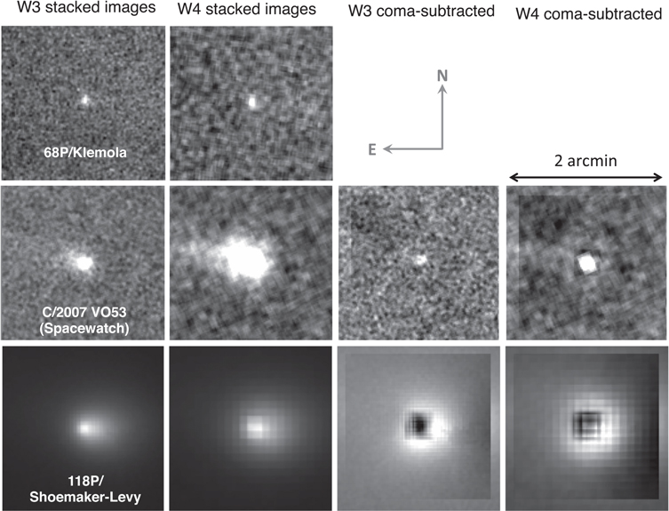
Figure 2. Examples of the comet coma subtraction technique. The images are oriented north up and east to the left and are 2 on a side. Comet 68P/Klemola (top row) exhibits no obvious coma, and the diameter estimate was derived from direct 11 aperture photometry on the stacked images. C/2007 VO53 (Spacewatch; central row) shows an example of coma subtraction on an active LPC. The remaining nucleus signal in the coma-subtracted W3 and W4 images was used to derive the diameter of the nucleus. Comet 118P/Shoemaker–Levy exhibited too complex of coma structure to successfully apply the coma subtraction technique. Comets that did not have successful coma subtraction were excluded from the nucleus size–frequency distribution analyses. A total of 2 out of the 56 LPCs and 7 out of the 108 SPCs yielded no nucleus size constraints, so that ∼94% yielded constraints.
Download figure:
Standard image High-resolution imageTable 2. Coma Subtraction Model Fit Parameters
| WISE Band | Model | Coma Fit Interval ( from Central Condensation) |
Comments |
|---|---|---|---|
| W3 | 1 | 8.5–20.0 | Least aggressive; fitted coma signal lowest |
| 2 | 7.0–19.0 | ||
| 3 | 7.0–15.0 | ||
| 4 | 2.0–13.0 | Most aggressive; fitted coma signal greatest | |
| 5 | No Subtraction, stacked image alone | No Coma apparent | |
| W4 | 1 | 7.0–15.0 | |
| 2 | 5.0–13.0 | ||
| 3 | 7.0–19.0 | Least aggressive; fitted coma signal lowest | |
| 4 | 3.0–16.0 | Most aggressive; fitted coma signal greatest | |
| 5 | No Subtraction, stacked image alone | No Coma apparent | |
Download table as: ASCIITypeset image
Table 3. Diameters and εfρ
| Design. | eta | eta_err | D[km] | Derr |
 [log cm] [log cm] |

|
W3CS Mod. | W4CS Mod. | Comments |
|---|---|---|---|---|---|---|---|---|---|
| SPCs | |||||||||
| 7Pa | 1.52 | 0.13 | 4.92 | 0.32 | 1.72 | 0.41 | 1, 3 | 2, 4 | |
| 9P | 0.65 | 0.05 | 5.95 | 0.24 | 2.20 | 0.38 | 5 | 5 | |
| LPCs | |||||||||
| C/2005 L3 | 4.05 | 0.12 | n/a | n/a | Too Dusty, no nucleus signal | ||||
| C/2006 OF2 | 12.54 | 2.67 | 3.11 | 0.09 | 1, 2, 4 | 1–4 | |||
Notes.
aIndicates that the comet was not detected by WMOPS, but found in co-moving image stacks. bSee Table 2. The first column lists the comet name. The dimensionless beaming parameter (eta) and associated uncertainty (eta_err) from the fits are also provided for those fits where eta was a free parameter. The "nan" values in the eta-related columns indicate that the beaming parameter was fixed (see text). Diameters (D) and their uncertainties (Derr) are reported in km units, while εfρ values and their associated uncertainties (σεfρ) are in base-10 log cm units. The "nan" value signal was too weak to constrain εfρ. Values of 0 for εfρ indicate no evidence of coma. The coma subtraction models for W3 and W4 that were used for the nucleus effective diameter fits, as listed in Table 2 and described in the text, are indicated by the W3CS and W4CS columns. Where diameter fits were previously published, the reference was given in these two columns. The "nan" values in these two columns indicate that the signal in that band was not used in the diameter fit, usually owing to the weak signal in that band. Comments regarding the fits and signal are listed in the last column.Only a portion of this table is shown here to demonstrate its form and content. A machine-readable version of the full table is available.
Download table as: DataTypeset image
The nucleus magnitudes and uncertainties for W3 and W4 are input to the thermal fits, yielding diameters and diameter uncertainties (Mainzer et al. 2011c). More often than not, the larger uncertainty in the photometry from the coma subtraction did not sufficiently restrict the beaming parameter in the thermal fits. Except where noted, therefore, most beaming parameters were set to 1.0, with an assumed uncertainty of 0.2, in line with the beaming parameter values found for other comets by Fernández et al. (2013). Those 56 nuclei that were successfully fit for the beaming parameter yielded an average value of 1.1 ± 0.2 for 20 LPCs and 1.1 ± 0.3 for 32 JFCs, excluding the Halley-type comets (Bauer et al. 2015) and active centaurs (Bauer et al. 2013) in our sample.
The extracted diameters were compared to the SST's Survey of the Ensemble Physical Properties of Cometary Nuclei (SEPPCon; Fernández et al. 2013) diameters and those derived from spacecraft (Figure 3) and were found to correspond to within a fractional mean of 0.25. Note that while three out of four spacecraft-encounter diameters match the NEOWISE-derived diameter values within the statistical uncertainties, NEOWISE observed 81P/Wild 2 while it was strongly active, so the coma subtraction method was less effective for these observations. While this point dominates the uncertainties of the spacecraft-encounter-derived diameter comparisons, we have included it still, since the sample of spacecraft-encounter comet nuclei is so small. As expected in a flux-limited survey, there is an apparent selection bias against comets with small diameter at large heliocentric distance (Figure 4).

Figure 3. Comparison of the NEOWISE-derived diameters with diameters derived from spacecraft encounters (dark-red triangles; A'Hearn et al. 2005, 2011; Duxbury et al. 2004; Soderblom et al. 2002 and Sierks et al. 2015) and SST (green triangles; Fernández et al. 2013). Vertical error bars represent the 1σ uncertainty based on the NEOWISE results, while horizontal uncertainty represents the uncertainties based on the comets' elongated shape for the spacecraft data and the uncertainties from Fernández et al. (2013) for the SST-derived diameters. The solid blue line represents a 1-to-1 correspondence. The data are consistent within the quoted uncertainty. The mean fractional offset between the NEOWISE and SST diameters is 0.22, and that between the NEOWISE and spacecraft-encounter diameters is 0.25.
Download figure:
Standard image High-resolution image
Figure 4. NEOWISE comet diameters vs. heliocentric distance at the time of observation by NEOWISE. The red triangles are JFCs, and the blue triangles are LPCs. The selection bias against small objects at large heliocentric distances is apparent, as well as inherent to a flux-limited survey.
Download figure:
Standard image High-resolution image3.2. Observed Undebiased Size Distributions
The population summaries of the comet sizes are shown in Figure 6, which presents a subsample of the observed cumulative SFDs for the two major dynamical types. In order to compare our raw diameter distributions with those in the literature, it was necessary to get a sense of the observed distributions down to at least the larger sizes. We therefore selected LPCs and JFCs observed within 4 au (Rh). The mean size for both the subsample and total sample of JFCs was 3 km in diameter. For the LPCs, the mean size for the subsample was 6 km, while for the total sample, the average was 8.5 km in diameter.
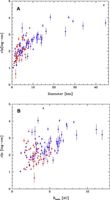
Figure 5. Diameter vs. εfρ (Panel A) and Rh vs. εfρ (Panel B). The red triangles represent the SPCs, while the blue triangles show the LPCs. A bifurcation or spread between the diameter and εfρ values exists out to sizes approaching 20 km. This effect is robust to debiasing, such that the quantity of dust ejected grows with diameter. Note that the εfρ values have no significant correlation with Rh, but at large distances there is an inherent observational selection effect where the survey is less sensitive to comets that generate smaller quantities of dust, i.e., those with smaller nuclei, at large distances.
Download figure:
Standard image High-resolution imageSFD fits to the raw observed subsamples are in agreement with Fernández et al. (2013) for the JFC comet population. For the number of comets, N, with diameter exceeding D, the SFD follows a power-law relation:  . The power-law parameter found from our data, β = −1.93 ± 0.06, closely matches the value obtained using the SST data by Fernández et al. (2013) of β = −1.92 ± 0.23. Furthermore, the median diameter is 3 km, which is midway between the Meech et al. (2004) median JFC size of 3.2 km and the Fernández et al. (2013) median of 2.8 km. The Meech et al. (2004) result for the LPC SFD slope parameter (β = −1.45 ± 0.05) for the subsample inside of 4 au also agrees well with the fit to our data (β = −1.44 ± 0.01). Our NEOWISE undebiased SFD for the JFC population shows a "knee" around 3–5.5 km and rollover below 4.3 km. Such features were observed by Fernández et al. (2013) as well.
3.3. Debiased Comet Populations
NEOWISE provides a data set that regularly samples the sky, uninterrupted by seeing, transparency, weather, or daytime, and so renders a data set that is uniquely suited to debiasing methodologies that compensate for coverage and sensitivity to constrain the underlying populations. Mainzer et al. (2011b) and Grav et al. (2012a, 2012b) provide examples of the debiasing techniques that may be employed to determine both nearby near-Earth object and more distant Hilda and Trojan asteroid populations, respectively. We employ similar techniques to remove the effects of systematic survey biases in the observed comets.
We start by constructing an accurate simulation of the NEOWISE survey that re-creates the sensitivity and per-exposure sky position footprint. Sample populations of LPCs and SPCs were then randomly distributed according to the orbital distributions of their respective populations, as in the solar system simulator (S3M) of Grav et al. (2011a). Input objects were then binned according to size, orbital inclination, eccentricity, perihelion distance, and heliocentric distance values. The number of objects detected in the simulated survey was determined, and their fractional detection rate was calculated in each bin and applied to the observed populations, identically binned. This yielded the total population in each bin and so allowed derivation of the debiased SFD and underlying total population.
The main difference between cometary and other small-body populations is that comets are active; therefore, a model representing their activity as a function of heliocentric distance, diameter, and days from perihelion was applied. We applied the following relation for εfρ (log cm units; Figure 5) and in turn derived the combined coma and nucleus flux:

where the fitted value of N(0, 0.25) is a normal distribution with a mean of 0 and a standard deviation of 0.5 (or variance of 0.25) added to match the uncertainties. We note, as stated in Figure 5, that the Kendall τ and the corresponding p-values for our sample of εfρ values compared to heliocentric distance out to 4 au are 0.16 and 0.052, respectively, which do not indicate significant confidence of a correlation. However, for the εfρ values compared to the square of the diameter values, τ = 0.6 and p < 1.E−7, respectively, indicating a strong correlation.
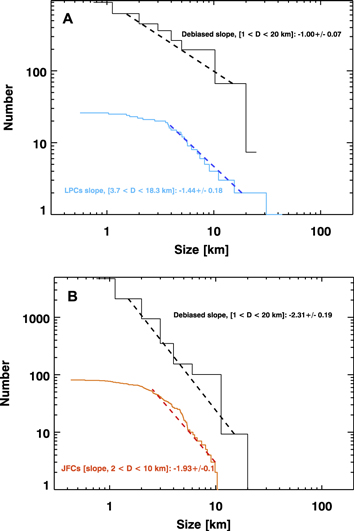
Figure 6. Undebiased SFD of the NEOWISE comets observed during the cryogenic mission (log scale). The total combined sample of LPCs (Panel A) and JFCs (Panel B) is shown. In order to obtain a raw, biased distribution down to diameters of ∼2 km for comparison to literature data sets, a subset of comets observed within 4 au was selected from the JFCs (orange histogram) and the LPCs (cyan histogram), and the linear fits are shown by the red and blue dashed lines, respectively. The debiased population is shown by the solid black line in each panel, with a linear slope fit shown with a dashed black line.
Download figure:
Standard image High-resolution image
The results of the debiasing are shown in Figure 6. Size bins spanning diameters of 25 km down to 0.75 km were used to derive SFD slopes, resulting in debiased power laws of β = −2.3 ± 0.2 for the JFCs and β = −1.0 ± 0.1 for the LPCs. The differences in slope became more significant after debiasing. For the debiased mean diameter in each sample, the ratio of the mean diameter for the LPCs to that of the JFCs is ∼1.6 (mean debiased LPC diameter of 2.1 km/mean debiased JFC diameter of 1.3 km). The debiased population has a larger number of smaller-diameter objects in both the LPC and JFC populations, as expected. However, the smallest size bin, 0.75 km (spanning 0.5–1 km diameters), roughly agrees with the β slope law fitted from the other bins, and we find no evidence of a deficiency of smaller-sized objects down to the ∼0.8 km diameter size range. The predicted size at which this may occur is ≤2 km (see Francis 2005 and Dones et al. 2015). It should be noted that the results in the smallest bin for each population are based on small-number statistics, as only a few subkilometer nuclei were measured for each population. Therefore, in interpreting the total number of objects in the comet populations, we use the next-largest 1.5 km bin to compare with the total numbers of the debiased populations from Oort (1950) and Francis (2005) for the LPCs and Brasser & Wang (2014) and Fernandez et al. (1999) for the JFCs. For the LPCs, we found 626 comets with nuclei ∼1.5 or greater in diameter out to 7 au, and 2116 JFCs. Our LPC debiased population is not dissimilar to that found by Everhart (1967) for the numbers out to 4 au, when scaling by diameter and perihelion distance. The debiased LPC population indicates that ∼7 comets >1 km in size passed within 1.5 au of the Sun over the course of a year, which is greater by a factor of 7.2 than the Oort (1950) results and by a factor of 2.6 than the Francis (2005) results. For the JFC populations, our ∼2100 comets compare with the Fernandez et al. (1999) estimates of a few thousand to 10,000 down to a similar size range, while it is about a factor of 7 greater than the Brasser & Wang (2014) estimate of ∼300 comets. However, the comparison with Brasser & Wang is not as straightforward owing to the fact that their limits are pinned to observed magnitudes and the differences in brightening models they employ, which may not be appropriate for the different wavelength regime of our data.
4. Discussion
Thermal-infrared observations from space-based platforms provide an effective means of determining the primary physical parameter, size, of small-body populations. The results of the undebiased NEOWISE cometary diameters affirm three of the key elements found in the SEPPCoN survey results for the JFCs, an SFD slope parameter of β = −1.93, the existence of a "knee" in the JFC size distribution near diameters of 4.3 km, and a median value for JFC cometary nucleus diameters near 3 km, also seen by Meech et al. (2004). However, it is important to note that this "knee" is not apparent in the debiased size–frequency distribution. Related populations, such as the Centaurs, have shown similar β values (Stansberry et al. 2008; Bauer et al. 2013; Licandro et al. 2016) in their observed SFDs. The moderately steeper debiased SFD slope of β = −2.3 is driven by the increase at the smaller size end of the population owing to the debiasing that also shows no lack of comets in the smaller nucleus size bins.
While a second value affirmed now by two surveys is the LPC observed SFD slope parameter, the debiased SFD slope value of β = −1.0 is even shallower. The LPC β parameter is distinct from the JFC β value, and considering that the population of LPCs may represent or be derived from the small bodies least altered by insolation processes, i.e., the Oort cloud objects, this may be a primordial feature of the LPCs. It thus could be emblematic of the scales at which these bodies formed. Morbidelli et al. (2008) have speculated that small bodies under 100 km in diameter are likely products of primordial collisions. Perhaps that is why the LPCs have a shallower SFD, while evolutionary processing, such as mass loss, has moved the JFCs and related bodies away from a similar β value.
Size and εfρ.—Large-grained dust particles from cometary comae can remain in the vicinity of the nucleus for years (Stevenson et al. 2014), and observations at infrared wavelengths tend to be more sensitive to the presence of larger grains (Bauer et al. 2008; Kramer 2014; Kramer et al. 2017). We thus expect the observed weaker correlation with distance as compared to the production of gas species such as CO or CO2 (Bauer et al. 2015). Other infrared dust studies find no correlation with dust production and the perihelion distance (Kelley et al. 2013). However, there is an apparent relation between εfρ and diameter for both populations we investigated, with a dispersion of about ±0.5 in log cm. We see a correlation that scales approximately with the square of the nucleus size (or nearly linearly with surface area). Hence, a constant fraction of active area may be common up to large sizes. We should not, then, expect larger comets to have a higher reflectance even for LPCs as compared to JFCs, since the trend is seen for both. However, no albedo values are reported here, since our simultaneous reflectance constraints are only available for the W1 band, where the signal is often too weak to reliably extract the coma using the same methodology as for W3 and W4. Furthermore, the variation in εfρ for comets with similarly sized nuclei at similar heliocentric distance dominates over the variation with heliocentric distance for the same individual objects.
The debiasing of comet populations facilitated by the NEOWISE observations yields unique insight into their structure and the role in the inner solar system's evolution. Proceeding along the methodology of Oort (1950) and using our debiased sample of ∼600 LPCs with nuclei >1 km in diameter out to 7 au, approximately seven LPCs per year pass within 1.5 au. Oort (1950) derives a population of 1.8 × 10¹¹ comets given a flux of ∼1 comet per year that comes within 1.5 au, and Francis (2005) derives approximately 5 × 10¹¹, so that our debiased sample would imply approximately 1.3 × 10¹² Oort cloud objects, nearly three times the Francis (2005) estimate based on data from the LINEAR survey.
5. Conclusions
- 1.In the course of analysis of our observed distributions, we find a cluster of comets with orbital elements near 100° inclination and perihelion distances near 2.5 au that may have been caused by the breakup of an object. This is the first such cluster associated with the distribution of LPCs.
- 2.
- 3.The debiased populations show a slightly steeper power-law slope relation for JFCs than the raw distribution and a significantly shallower distribution slope for the LPCs. We suspect that the more shallow size distribution in the LPCs is primordial from their era of formation, rather than evolutionary, but that the steeper β value for JFCs is dominated by evolutionary mass-loss processes over time that have reduced the size of all members and maybe even destroyed the smallest members. The debiased populations maintain that the average size for the JFCs is smaller than for the LPCs, but the difference is a factor of 1.6, rather than the factor of 2 seen in the raw distributions, though the difference is still significant.
- 4.There is no apparent drop-off in the numbers of either the LPC or JFC populations at smaller size in the debiased population. However, as the debiased distribution in the smallest size bin is based on small-number statistics, a turnover at small sizes cannot be ruled out or confirmed for either class.
- 5.
This article makes use of data products from the Wide-field Infrared Survey Explorer, a joint project of the University of California, Los Angeles, and the Jet Propulsion Laboratory/California Institute of Technology, funded by the National Aeronautics and Space Administration. This article also makes use of data products from NEOWISE, which is a project of JPL/Caltech, funded by the Planetary Science Division of NASA. The material is based in part on work supported by NASA through the NASA Astrobiology Institute under Cooperative Agreement no. NNA09DA77A issued through the Office of Space Science. E.A.K. and R.A.S. were supported by the NASA Postdoctoral Program. We thank the Astronomical Journal editor for the very helpful comments regarding manuscript drafts and the anonymous reviewer for providing valuable comments, both of whom greatly improved the paper content.