


ABSTRACT
We report a new study of the V i atom using a combination of time-resolved laser-induced fluorescence and Fourier transform spectroscopy that contains newly measured radiative lifetimes for 25 levels between 24,648 cm−1 and 37,518 cm−1 and oscillator strengths for 208 lines between 3040 and 20000 Å from 39 upper energy levels. Thirteen of these oscillator strengths have not been reported previously. This work was conducted independently of the recent studies of neutral vanadium lifetimes and oscillator strengths carried out by Den Hartog et al. and Lawler et al., and thus serves as a means to verify those measurements. Where our data overlap with their data, we generally find extremely good agreement in both level lifetimes and oscillator strengths. However, we also find evidence that Lawler et al. have systematically underestimated oscillator strengths for lines in the region of 9000 ± 100 Å. We suggest a correction of 0.18 ± 0.03 dex for these values to bring them into agreement with our results and those of Whaling et al. We also report new measurements of hyperfine structure splitting factors for three odd levels of V i lying between 24,700 and 28,400 cm−1.
Export citation and abstract BibTeX RIS
1. INTRODUCTION
Studies of iron-group elements have long been an important part of astronomy and astrophysics. Due to their large binding energy per nucleon, they are both the heaviest elements that can be produced through nuclear fusion in stellar cores, and the lightest elements produced through the decay of heavy elements by nuclear fission. As a result, iron-group elements are relatively more abundant in stellar atmospheres than might otherwise be expected, forming what is known as the "iron peak."
In addition to this, partially filled 3d shells in their atomic structure lead to extremely line-rich spectra. The Fe i spectrum, for example, contains up to 10,000 lines that can be observed in the laboratory, spanning a region from the near infrared to the vacuum ultraviolet. Consequently, most of the opacity we observe in stars is due to iron-group elements.
In recent years, we have undertaken experimental measurements of oscillator strengths and level lifetimes in iron-group elements to improve models of stellar and solar spectra. To date, this survey has included Fe (Ruffoni et al. 2013, 2014; Den Hartog et al. 2014b), Mn (Blackwell-Whitehead & Bergemann 2007; Blackwell-Whitehead et al. 2011), Co (Bergemann et al. 2010), and Ti (Blackwell-Whitehead et al. 2006). In this paper, we turn our attention to neutral vanadium (V i).
The most notable previous studies of V i experimentally measured oscillator strengths were conducted by Doerr et al. (1985) and Whaling et al. (1985), and more recently by Lawler et al. (2014) and Den Hartog et al. (2014a). In general, the lifetimes and log(gf) values reported in these papers are of extremely good quality, but nonetheless the database remains incomplete, and historical values are frequently quoted with large uncertainties. In particular, astronomers have requested improvements be made to log(gf) values of neutral vanadium in the region 3500–8000 Å to improve modeling of the vanadium abundance in the Sun (M. Bergemann 2009, private communication).
Here, we report the results of a new, independent set of measurements of level lifetimes and oscillator strengths (log(gf)), obtained through a collaboration between Imperial College, Lund Laser Center, and Lund Observatory, which also serve as a means to assess the reliability of the data in the literature. As has become standard practice for such work, our new level lifetimes were obtained by time-resolved laser-induced fluorescence (TR-LIF), and log(gf) values found by combining these lifetimes with branching fractions, measured by high-resolution Fourier transform (FT) spectroscopy.
Overall, we find that previously published lifetimes and log(gf) values for V i are typically of good quality, especially those published by Lawler et al. (2014) and Den Hartog et al. (2014a) using the same techniques adopted in this study. However, by quantitatively comparing log(gf) values from Doerr et al. (1985), Whaling et al. (1985), Lawler et al. (2014), and this study, we have been able to highlight and suggest corrective action for a number of problems that appear in the literature. These are discussed in Section 3. We also compare theoretically calculated log(gf) values of Kurucz (2007) and recent results of Wang et al. (2014), which combine measured lifetimes and theoretical branching fractions, with our new data, and confirm that experimentally measured log(gf) values are more reliable where these exist. Additionally, we provide log(gf) values for 13 lines that have not been reported in any previous study, nine of which are in the infrared at wavelengths longer than 1.6 μm, which was the longest wavelength for any previously reported log(gf) value in V i (Whaling et al. 1985).
2. EXPERIMENTAL PROCEDURES
2.1. Radiative Lifetime Measurements
The experimental set-up used for our radiative lifetime measurements is shown schematically in Figure 1. A pure vanadium foil was placed on a rotating target in a vacuum chamber at a pressure between 10−4 and 10−3 Pa. This was then irradiated perpendicularly by ablation pulses of 10 ns duration and energies between 2 and 10 mJ, emitted from a Nd:YAG laser (Continuum Surelite) of 532 nm wavelength at a repetition rate of 10 Hz. These pulses entered the top of the vacuum system through a fused-silica window, and were focused vertically onto the surface of the rotating vanadium foil, producing a plasma of both neutral and ionized atoms that expanded into an interaction zone at the center of the chamber, about 10 mm above the foil. The ionized atoms traverse the chamber much faster than the neutrals, meaning that after a short delay, the plasma in the interaction zone contains only neutral atoms. At this moment, an excitation laser beam from a tunable nanosecond laser system intersects the plasma at right angles. This beam was linearly polarized and tuned in wavelength to the resonant transition of an upper state of interest.

Figure 1. Schematic diagram showing the main components of the TR-LIF apparatus used in this study. Solid lines between components indicate electrical connections and dashed lines represent light paths. The names of components with abbreviated labels are given in full in the text.
Download figure:
Standard image High-resolution imageThe tunable laser system consisted of an injection-seeded and Q-switched Nd:YAG laser (Continuum NY-82), a stimulated Brillouin scattering (SBS) temporal compressor, a DCM dye laser (Continuum Nd-60), a potassium dihydrogen phosphate (KDP) crystal, retarding plate (RP) and β-barium borate (BBO) crystal, and a stimulated Stokes Raman scattering (SSRS) cell.
The Nd:YAG seeded laser produced pulses of light at 532 nm wavelength, 8 ns duration, and 400 mJ energy, at a repetition rate of 10 Hz. These pulses were shortened in length to approximately 1 ns duration using an SBS compressor, and then sent to pump a DCM dye laser. To obtain the ultraviolet radiation needed to excite the vanadium atoms, light from the dye laser was passed through a frequency-doubling KDP crystal, producing second harmonic radiation that was mixed with the fundamental laser frequency in a BBO crystal to produce light at the third harmonic frequency. Finally, to expand the spectral range of the laser light, both the second and third harmonic radiation was focused onto a SSRS hydrogen cell at a pressure of 106 Pa, in which different orders of stimulated Stokes and anti-Stokes Raman scattering were produced.
Depending on the excitation requirements of a particular measurement, the appropriate component of the excitation laser was selected with a CaF2 Pellin–Broca (PB) prism, passed through two apertures and sent horizontally into a vacuum chamber where it struck the expanding plasma produced by the ablation laser. The two Nd:YAG lasers were controlled externally by a digital delay generator (Stanford Research Systems Model 535), which adjusted the delay between the ablation and excitation laser pulses, ensuring that the excitation laser met with the vanadium plasma only after the fast moving ionized atoms had traversed the laser interaction zone.
Fluorescence from the spontaneous decay of the targeted excited levels was focused by a fused-silica lens onto the entrance slit of a 1/8 m monochromator (resolution 6.4 nm mm−1), that was used as a filter to select a particular fluorescence line and to block stray light. This selected light was then detected by a Hamamatsu 1564U microchannel-plate photomultiplier tube (PMT, 200 ps rise time and sensitive between 200 and 600 nm), which was connected to a digital transient oscilloscope (Tektronix Model DSA 602), triggered by a Thorlabs SV2-FC photodiode (120 ps rise time) driven by a reflection from the excitation laser beam. These fluorescence signals were averaged in the oscilloscope and sent to a computer, where the level radiative lifetimes were measured. For the shorter lifetimes the temporal shape of the exciting laser pulses was recorded after the ablation beam was blocked and the decay curves then analyzed by deconvolving the observed signal and the laser pulse using the computer program DECFIT (Palmeri et al. 2008). The longer lifetimes were obtained by fitting a single exponential decay, and a background function, to the region after the pulse had expired.
Many systematic effects were considered and accounted for. A static magnetic field of approximately 100 G, provided by a pair of Helmholtz coils surrounding the laser interaction zone, was used to eliminate potential Zeeman quantum beat effects for long-lived states. Flight-out-of-view effects are also important, particularly for long lifetimes. During the experiment, the position and width of the monochromator entrance slit and the delay times between the ablation and the excitation pulses were adjusted to identify and eliminate the possible influence of such flight-out-of-view effects.
To make sure that the experimental lifetimes were not affected by collisions and radiative trapping—a particular concern when the delay between ablation and excitation pulses is short—the intensity of the ablation pulse was varied and the delay time adjusted within the range 2.8–5.5 μs, changing the plasma atomic density and temperature at the time of excitation. The resulting LIF signal intensities varied, but the lifetime values were found to be nearly constant, implying that the effects of collisional quenching and radiation trapping were negligible.
To avoid saturation effects and to ensure that the response of the detection system is linear, the fluorescence signals were detected with different neutral density filters inserted in the path of the exciting laser light.
A smooth fluorescence decay curve was obtained for each lifetime measurement by averaging fluorescence photons from 1000 pulses to obtain a sufficiently high signal-to-noise ratio (S/N). Between 10 and 20 curves were recorded for each level under the different experimental conditions listed above, and the averaged measured lifetime taken as the final value reported in Table 1. The errors quoted include the statistical scattering between the different recordings and different curve fittings, as well as any remaining systematic effects.
Table 1. Radiative Lifetimes for V i Levels with log(gf) Values Reported in Table 4
| Configuration | Term | J | Energy (cm−1)a | Measured Lifetimes, τ (ns) | |||
|---|---|---|---|---|---|---|---|
| This Study | Whalingb | Den Hartogc | Other LIF Values | ||||
| 3d3 (4F) 4s4p (3P) | z6D | 1/2 | 18085.952 | ⋯ | 390 ± 40 | 407.0 ± 20.4 | ⋯ |
| 3d3 (4F) 4s4p (3P) | z6D | 3/2 | 18126.250 | ⋯ | 395 ± 40 | 411.0 ± 20.6 | ⋯ |
| 3d3 (4F) 4s4p (3P) | z6D | 5/2 | 18198.091 | ⋯ | 395 ± 40 | 410.0 ± 20.5 | ⋯ |
| 3d3 (4F) 4s4p (3P) | z6D | 7/2 | 18302.280 | ⋯ | 385 ± 40 | 406.0 ± 20.3 | ⋯ |
| 3d3 (4F) 4s4p (3P) | z6D | 9/2 | 18438.044 | ⋯ | 370 ± 40 | 393.0 ± 19.7 | ⋯ |
| 3d3 (4F) 4s4p (3P) | z4D | 1/2 | 20606.467 | ⋯ | 86 ± 3 | 84.7 ± 4.2 | ⋯ |
| 3d3 (4F) 4s4p (3P) | z4D | 3/2 | 20687.769 | ⋯ | 83 ± 3 | 86.4 ± 4.3 | ⋯ |
| 3d3 (4F) 4s4p (3P) | z4D | 5/2 | 20828.481 | ⋯ | 89 ± 3 | 88.6 ± 4.4 | ⋯ |
| 3d3 (4F) 4s4p (3P) | z4D | 7/2 | 21032.503 | ⋯ | 92.5 ± 3 | 91.3 ± 4.6 | ⋯ |
| 3d4 (5D) 4p | z6P | 3/2 | 24648.114 | 27.3 ± 1.5 | ⋯ | 28.4 ± 1.4 | ⋯ |
| 3d4 (5D) 4p | z6P | 5/2 | 24727.841 | 27.4 ± 1.5 | ⋯ | 28.2 ± 1.4 | ⋯ |
| 3d4 (5D) 4p | z6P | 7/2 | 24838.578 | 26.6 ± 1.5 | ⋯ | 28.1 ± 1.4 | ⋯ |
| 3d4 (5D) 4p | z4P | 1/2 | 24770.673 | 23.3 ± 1.0 | 24 ± 1 | 24.7 ± 1.2 | ⋯ |
| 3d4 (5D) 4p | z4P | 3/2 | 24915.151 | ⋯ | 24 ± 1 | 25.6 ± 1.3 | ⋯ |
| 3d4 (5D) 4p | z4P | 5/2 | 25131.002 | ⋯ | 25 ± 1 | 25.4 ± 1.3 | ⋯ |
| 3d4 (5D) 4p | y6F | 1/2 | 24789.401 | 9.2 ± 0.3 | ⋯ | 9.4 ± 0.5 | ⋯ |
| 3d4 (5D) 4p | y6F | 3/2 | 24830.221 | 8.9 ± 0.3 | ⋯ | 9.2 ± 0.5 | ⋯ |
| 3d4 (5D) 4p | y6F | 5/2 | 24898.804 | 8.8 ± 0.3 | ⋯ | 9.1 ± 0.5 | ⋯ |
| 3d4 (5D) 4p | y6F | 7/2 | 24992.909 | 8.8 ± 0.3 | ⋯ | 9.1 ± 0.5 | ⋯ |
| 3d4 (5D) 4p | y6F | 9/2 | 25111.473 | 8.9 ± 0.3 | ⋯ | 9.1 ± 0.5 | ⋯ |
| 3d4 (5D) 4p | y6F | 11/2 | 25253.457 | 8.7 ± 0.3 | ⋯ | 9.0 ± 0.5 | ⋯ |
| 3d4 (5D) 4p | y4D | 1/2 | 26182.637 | ⋯ | 12.3 ± 0.5 | 12.4 ± 0.6 | 12.3 ± 0.7d; 12.7 ± 0.9e |
| 3d4 (5D) 4p | y4D | 3/2 | 26249.476 | ⋯ | 12.3 ± 0.5 | 12.5 ± 0.6 | 11.9 ± 0.7d; 12.9 ± 0.9e |
| 3d4 (5D) 4p | y4D | 5/2 | 26352.634 | ⋯ | 12.4 ± 0.5 | 12.5 ± 0.6 | 12.4 ± 0.7d; 13.3 ± 0.9e |
| 3d4 (5D) 4p | y4D | 7/2 | 26480.286 | 12.3 ± 0.5 | 12.5 ± 0.5 | 12.6 ± 0.6 | 12.2 ± 0.7d; 13.8 ± 1.0e |
| 3d4 (5D) 4p | y6D | 1/2 | 26397.633 | ⋯ | 7.7 ± 0.6 | 8.2 ± 0.4 | 8 ± 0.4d |
| 3d4 (5D) 4p | y6D | 3/2 | 26437.754 | ⋯ | 7.8 ± 0.5 | 8.1 ± 0.4 | 8.1 ± 0.4d |
| 3d4 (5D) 4p | y6D | 5/2 | 26505.953 | ⋯ | 7.9 ± 0.5 | 8.1 ± 0.4 | 7.9 ± 0.4d |
| 3d4 (5D) 4p | y6D | 7/2 | 26604.807 | ⋯ | 7.8 ± 0.5 | 8.0 ± 0.4 | 8 ± 0.4d; 7.8 ± 0.5f |
| 3d4 (5D) 4p | y6D | 9/2 | 26738.323 | 7.9 ± 0.4 | 7.9 ± 0.5 | 8.0 ± 0.4 | 7.8 ± 0.4d |
| 3d3 (4P) 4s4p (3P) | x6D | 1/2 | 28313.626 | 35.5 ± 2.0 | ⋯ | 35.6 ± 1.8 | 36.4 ± 2.5f |
| 3d3 (4P) 4s4p (3P) | x6D | 3/2 | 28368.753 | 36.5 ± 2.0 | ⋯ | 35.9 ± 1.8 | 36.5 ± 2.6f |
| 3d3 (4P) 4s4p (3P) | x6D | 5/2 | 28462.177 | 37.0 ± 2.0 | ⋯ | 36.6 ± 1.8 | 37.7 ± 2.6f |
| 3d3 (4P) 4s4p (3P) | x6D | 7/2 | 28595.637 | 37.5 ± 2.0 | ⋯ | 37.7 ± 1.9 | 38.7 ± 2.7f |
| 3d3 (4P) 4s4p (3P) | x6D | 9/2 | 28768.142 | 40.0 ± 2.0 | ⋯ | 39.5 ± 2.0 | 39.7 ± 2.8f |
| 3d3(2G) 4s4p (3P) | y4G | 5/2 | 30635.580 | 72.0 ± 4.0 | ⋯ | 72.4 ± 3.6 | 76.4 ± 4.2f; 74 ± 5.0g |
| 3d3 (4F) 4s4p (1P) | w4F | 3/2 | 32738.130 | 4.6 ± 0.3 | ⋯ | 4.5 ± 0.2 | ⋯ |
| 3d3 (4F) 4s4p (1P) | w4F | 5/2 | 32846.822 | 4.1 ± 0.3 | ⋯ | 4.1 ± 0.2 | ⋯ |
| 3d3 (4F) 4s4p (1P) | w4F | 7/2 | 32988.845 | 4.4 ± 0.3 | ⋯ | 4.2 ± 0.2 | ⋯ |
| 3d3 (4F) 4s4p (1P) | w4F | 9/2 | 33155.331 | 4.1 ± 0.2 | ⋯ | 4.0 ± 0.2 | ⋯ |
| 3d4 (3H) 4p | z4I | 9/2 | 37285.057 | ⋯ | ⋯ | 25.8 ± 1.3 | ⋯ |
| 3d4 (3H) 4p | z4I | 11/2 | 37315.932 | 13.5 ± 0.8 | ⋯ | 14.3 ± 0.7 | ⋯ |
| 3d4 (3H) 4p | z4I | 13/2 | 37404.329 | 11.9 ± 0.8 | ⋯ | 12.5 ± 0.6 | ⋯ |
| 3d4 (3H) 4p | z4I | 15/2 | 37518.445 | 11.6 ± 0.8 | ⋯ | 12.3 ± 0.6 | ⋯ |
Notes.
aThorne et al. (2011). bWhaling et al. (1985). cDen Hartog et al. (2014a). dDoerr et al. (1985). eRudolph & Helbig (1982). fWang et al. (2014). gXu et al. (2006).A machine-readable version of the table is available.
Download table as: DataTypeset image
2.2. log(gf) Measurements
Accurate experimental log(gf) values can be obtained by combining the radiative lifetime of a level, τ, with radiative transition branching fractions (BFs) derived from the relative intensity of all spectral lines emanating from transitions linked to that level (Huber & Sandeman 1986). For the log(gf) values reported in Table 4, BFs were obtained from V i emission line spectra measured by FT spectrometry in several overlapping regions between 2000 cm−1 and 34,500 cm−1 (between 5000 and 290 nm). These spectra are listed in Table 2.
Table 2. Spectra Used in this Analysis
| Spectrum | Spectral | Lamp I | Detector | Filter | Resolution | Spectrum Filename |
|---|---|---|---|---|---|---|
| Range (Å) | (mA) | (cm−1) | ||||
| A (Lund) | 50000–2000 | 500 | InSb | None | 0.02 | V09120416 (2009 Dec 4 ) |
| B (Lund) | 8696–4505 | 500 | R1477-06 PMT | Na | 0.03 | V0911271 (2009 Nov 27) |
| C (Lund) | 8696–4505 | 200 | R1477-06 PMT | Na | 0.03 | V0911273 (2009 Nov 27) |
| D (IC) | 7692–4651 | 500 | R928 PMT | GG475, Na | 0.037 | V130520A, scans 4 to 57 (2013 May 20) |
| E (IC) | 5952–3509 | 500 | R11568 PMT | WG335, Na | 0.037 | V130517A, scans 28 to 49 (2013 May 17) |
| F (IC) | 4808–2899 | 500 | R11568 PMT | BG3 | 0.037 | V130516, scans 2 to 16 (2013 May 16) |
| G (IC) | 4808–2899 | 300 | R11568 PMT | BG3 | 0.037 | V130516, scans 17 to 32 (2013 May 16) |
Note.
aHolographic notch filter blocking light in a 10 nm region centered at 632.8 nm (15802 cm−1). This removes scattered light from the He–Ne laser used to measure the difference in optical path length of the two branches of the FT spectrometer.Download table as: ASCIITypeset image
Spectra A to C were measured at Lund Observatory, Sweden, on a Bruker IFS-125HR infrared FT spectrometer, which has a resolving power R = 106 at 5 μm. The V i emission was generated from a vanadium cathode (99.9% pure) mounted in a water-cooled hollow cathode lamp (HCL) running at currents of up to 500 mA in a neon atmosphere at a pressure between 220 and 230 Pa. Each of the three spectra were constructed from up to 20 repeated measurements, coadded together to improve the S/N of lines of interest. In spectrum B many target lines were observed to be very strong (S/N ≳ 1000). Spectrum C was thus taken across the same spectral range, but at a lower lamp current of 200 mA, to verify that these strong lines were free from any self-absorption.
The spectrum of a tungsten lamp calibrated by the Swedish National Laboratory—with spectral radiance known to ±3% between 400 and 800 nm, and ±5% between 800 and 2500 nm—was also measured before each of the listed vanadium spectra to obtain the response function of the spectrometer as a function of wavenumber. The response functions are shown in Figure 2.
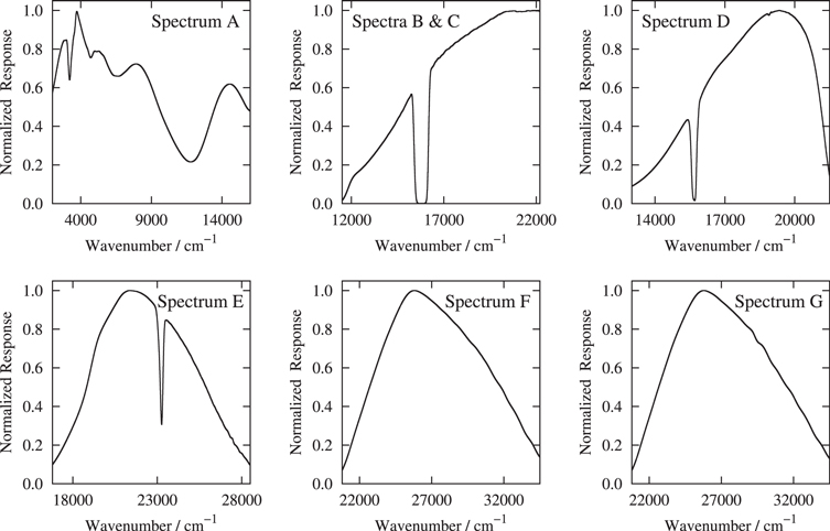
Figure 2. Spectrometer response functions for the seven spectra listed in Table 2. The plotted region in each panel corresponds to the spectral region that was used for analysis, i.e., the region where accurate intensity calibration could be obtained. The response functions for spectra B and C were identical within noise and are overplotted in the same panel.
Download figure:
Standard image High-resolution imageSpectra D to G were measured at Imperial College (IC) London, UK, on a Chelsea Instruments FT spectrometer based on an IC prototype design (Thorne et al. 1987; Thorne 1996) with spectral range down to 135 nm. The V i emission was generated using an HCL of similar design to that employed at Lund, again operated at currents of up to 500 mA, but in an argon atmosphere at a pressure 30 Pa. Spectrum F contained many target lines with S/N ≳ 1000, so as with the Lund measurements, Spectrum G was acquired under similar conditions, but with a lower lamp current of 300 mA, to allow any effects from self-absorption to be corrected.
The spectrometer response functions for spectra D and E were again obtained from a calibrated W lamp, measured before and after each HCL measurement. Uncertainties in the relative spectral radiance of the W lamp used at IC, and calibrated by the UK National Physical Laboratory (NPL), do not exceed ±1.4% between 410 and 800 nm, and rise to ±2.8% at 300 nm. Spectra F and G extended too far into the ultraviolet to be calibrated from the measurement of a W standard lamp alone. For these spectra, an additional measurement was made of a deuterium lamp before and after each HCL measurement. This lamp was calibrated by the Physikalisch-Technische Bundesanstalt (PTB), Germany, and has a relative spectral radiance known to ±7% between 170 and 410 nm. The spectrometer response function obtained from this lamp was combined with that from the W lamp such that the final response function used to calibrate the vanadium line spectrum was defined at longer wavelengths by the W lamp and at shorter wavelengths by the deuterium lamp. The response functions for spectra D to G are also shown in Figure 2.
Of the 39 upper energy levels for which we report log(gf) values, 25 linked to lower energy levels through transitions that produced spectral lines contained entirely within the range of a single spectrum listed in Table 2. For the remaining levels, the spectral lines spanned at least two spectra. In these cases, the intensities of lines observed in regions of overlap between any two spectra were compared, and the intensity scale of all required spectra adjusted to match the spectrum that contributed most to the total upper-level branching fraction. This process of intensity calibration of several spectra overlapping in wavelength is given in more detail in Pickering et al. (2001a, 2001b).
The predicted transitions from each target upper energy level to lower energy levels were taken from the semi-empirical calculations of Kurucz (2007). Emission lines associated from these transitions were then identified in our vanadium HCL spectra, and the XGREMLIN package (Nave et al. 2015) was then used for making center-of-gravity (COG) fits to the observed profiles (Thorne et al. 2011). The V i spectrum is affected by hyperfine structure (Thorne et al. 2011), and all hyperfine components of a given line were included in the COG fit to obtain the total observed intensity of the line, as shown in the example in Figure 3.
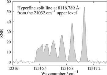
Figure 3. Example COG fit to a hyperfine split line. The total intensity of the line is the shaded area, which is the integrated intensity of the spectrum between two markers. These markers were placed on each side of the line at the point where the intensity was perceived to drop below the spectral noise.
Download figure:
Standard image High-resolution imageThe results from the XGREMLIN line-fitting process (relative line intensities, line S/N) together with the experimental spectra were then transferred to the FAST package (Ruffoni 2013), which was then used to calculate the BFs.

where the subscript u denotes a target upper energy level, and ul, a transition from this level to a lower level, l, resulting in a line of intensity Iul.
Spectra B and F were preferred over spectra C and G, respectively, for lines in those spectral regions, because the higher HCL running current produced lines of greater S/N. However, in cases where any one hyperfine component of a line was observed to have a very large S/N, the BF measurement was repeated using the line profile observed in spectrum C or G to ensure that the final BF value was not affected by self-absorption.
Lines that were too weak to be observed—typically those predicted by Kurucz (2007) to contribute less than 1% of the total BF—were not considered, nor were lines that were either blended or outside the measured spectral range. Their predicted contribution to the total BF was assigned to a "residual" value, which was used to scale the sum over l of Iul. The predicted BFs of Kurucz (2007) are used because we found these to be more reliable than those of Wang et al. (2014) due to the strong cancellation effect reported by Wang et al. (2014) affecting some of the transitions, in particular those depopulating the lowest excited odd-parity levels. Figure 4 shows comparisons of our measured BFs with those of Kurucz (2007) and Wang et al. (2014). For the majority of levels for which we report BFs, the residuals are less than 1%, with the least complete set being 94%.

Figure 4. Comparison between BF values from this work and theoretical values of Kurucz (2007; left panel) and Wang et al. (2014; right panel).
Download figure:
Standard image High-resolution imageThe final BF values were then combined with the measured radiative lifetime of upper level u to obtain the transition probability, or Einstein A coefficient of the transition:

This is equivalent to its log(gf) value, which was obtained from the expression (Thorne et al. 2007)

where λ is the wavelength of the line in nm, and gu the statistical weight of the upper level.
The uncertainty in each log(gf) value quoted in Table 4 arose from a combination of the uncertainty in its BF and that in its upper-level lifetime.
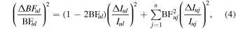
where ΔIul is the sum of uncertainties in intensity of a line due to its measured S/N, the uncertainty in calibrating the intensity scale of the spectrum, and the uncertainty in the factor used to place two overlapping spectra on a common intensity scale (Ruffoni 2013). The uncertainty in Aul, following from Equation (2), is then given by

where Δτul is the uncertainty in the upper-level lifetime. Thus, the uncertainty in log(gf) of a particular line is given by

2.3. The Use of Hyperfine Structure Splitting in Blended Lines to Determine BFs
During the analysis it was found that in the cases of three transitions of interest it was possible to find BF values for transitions that were blends with other V i transitions by fitting the observed hyperfine structure (hfs) of the lines involved in the blends using the hfs Ahfs splitting factor of each energy level involved in the transition. The three transitions appeared in two blended features: at 4408 Å (22,677 cm−1) with transitions  and
and 

 and at 3813 Å (26,215 cm−1) with transitions expected to contribute significantly to the blend

 and
and  .
.
An example of one of the blended features is given in Figure 5. However, initially in each case only one of the two Ahfs factors involved in a transition was known, and so in order to estimate the relative intensity of each transition, the unknown Ahfs factor had to be found. Following methods reported in Pickering (1996) and Blackwell-Whitehead et al. (2005), new Ahfs factors were found by analysing other spectral lines observed that involve the same level (full details may be found in Holmes 2016). The Ahfs factors together with their uncertainties used to find the BFs of three transitions are shown in Table 3. The value for level  has not previously been published and is new. Our new measurements of Ahfs for levels
  and
and  are compared with those recently published by Güzelçimen et al. (2014) and are found to have reasonable agreement considering the given experiment uncertainties.
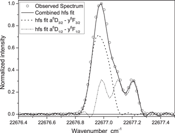
Figure 5. Blended feature at 4408 Å (22,677 cm−1) observed in FT spectrum G of a vanadium hollow cathode lamp run in argon at a pressure of 30 Pa, current 300 mA, with the two fitted transitions contributing to the blend.
Download figure:
Standard image High-resolution imageTable 3. V i New and Previously Published Hyperfine Structure Splitting Factors, Ahfs and Bhfs, Used in Fitting of the 22,677 and 26,215 cm−1 Blended Features
| Level | Level Energy | Ahfs | Bhfs | Source |
|---|---|---|---|---|
| (cm−1) | (×10−3 cm−1) | (×10−3 cm−1) | ||

|
137.383 | 10.7159 ± 0.0001 | 0.132 ± .001 | CPGC |

|
2112.282 | 25.0685 ± 0.0002 | 0 | CPGC |

|
2153.221 | 13.5309 ± 0.0001 | −0.2330 ± 0.0004 | CPGC |

|
24789.401 | 28.3a ± 0.4 | 0 | new |

|
24830.221 | 7.1a ± 0.2 | 0 | new |

|
26352.634 | 0.51 ± 0.03 | 0 | PBAG |

|
28368.753 | 22.5 ± 0.2 | 0 | new |
Notes. Source column: source of published hyperfine structure splitting factors: CPGC, Childs et al. (1979); PBAG, Palmeri et al. (1995); "new," newly found in this work.
aWe note that Güzelçimen et al. (2014) also report new values of Ahfs of (27.9 ± 0.6) × 10−3 cm−1 for the level at 24,789 cm−1 and (6.7 ± 0.1) × 10−3 cm−1 for the level at 24830 cm−1. Energy level values are from Thorne et al. (2011).Download table as: ASCIITypeset image
3. RESULTS
Table 1 lists the energy levels of V i included in this study along with their lifetimes. For 25 of these levels, we provide new lifetime values from our TR-LIF measurements, which agree with the previous work of Whaling et al. (1985), Doerr et al. (1985), or Den Hartog et al. (2014a), where those studies overlap. The close agreement we observe with the recent extensive study of V i lifetimes by Den Hartog et al. (2014a) is not surprising given the maturity of the TR-LIF set-ups at Wisconsin and at Lund. However, it is still reassuring that two independent studies of lifetimes for these levels produce consistent results.
Branching fraction measurements were attempted for all levels listed in Table 1 and completed for 39 of them. These include 21 levels for which we measured new lifetimes and an additional 18 levels of similar configuration and/or energy, which were measurable from our FT spectra. These BFs were then combined with the level lifetimes from this study, where they existed, or the lifetimes with the lowest uncertainty from either Whaling et al. (1985) or Den Hartog et al. (2014a) in all other cases, to produce the log(gf) values reported in Table 4. The remaining five levels in Table 1 were omitted from the log(gf) determinations because one or more important lines were blended or observed with only a very low a S/N, or because important lines spanned more than one spectrum listed in Table 2 but were too far separated to be put on a common intensity scale.
Table 4. Experimental log(gf) Values for 208 Lines of V i from this Study Sorted by Upper Level Energy
| λair (Å) | Upper Level | Lower Level | BF (%) | UBF | log(gf) Values | ||||||||
|---|---|---|---|---|---|---|---|---|---|---|---|---|---|
| E (cm−1) | J | E (cm−1) | J | This work | This work | Lawler | Whaling | Doerr | |||||
| 5527.618 | 18085.952 | 0.5 | 0.000 | 1.5 | −3.99 ± 0.03 | −4.00 ± 0.07 | |||||||
| 6258.571 | 18085.952 | 0.5 | 2112.282 | 0.5 | 29.8 | 1.3 | −2.07 ± 0.02 | −2.06 ± 0.02 | −2.04 ± 0.04 | ||||
| 6274.652 | 18085.952 | 0.5 | 2153.221 | 1.5 | 69.8 | 0.5 | −1.69 ± 0.02 | −1.70 ± 0.02 | −1.67 ± 0.05 | ||||
| 5515.329 | 18126.250 | 1.5 | 0.000 | 1.5 | −3.96 ± 0.03 | −3.93 ± 0.06 | |||||||
| 5557.450 | 18126.250 | 1.5 | 137.383 | 2.5 | 0.58 | 8.3 | −3.47 ± 0.03 | −3.45 ± 0.02 | −3.43 ± 0.04 | ||||
| 6242.822 | 18126.250 | 1.5 | 2112.282 | 0.5 | 44.4 | 0.8 | −1.60 ± 0.02 | −1.59 ± 0.02 | −1.55 ± 0.03 | ||||
| 6285.160 | 18126.250 | 1.5 | 2220.156 | 2.5 | 49.5 | 0.7 | −1.55 ± 0.02 | −1.54 ± 0.02 | −1.51 ± 0.03 | ||||
| 5535.344 | 18198.091 | 2.5 | 137.383 | 2.5 | 0.49 | 10.6 | −3.54 ± 0.05 | −3.57 ± 0.03 | −3.61 ± 0.04 | ||||
| 5592.960 | 18198.091 | 2.5 | 323.432 | 3.5 | 0.74 | 7.7 | −3.24 ± 0.03 | −3.21 ± 0.03 | −3.23 ± 0.04 | ||||
| 6230.798 | 18198.091 | 2.5 | 2153.221 | 1.5 | 49.0 | 0.7 | −1.38 ± 0.02 | −1.37 ± 0.02 | −1.34 ± 0.03 | ||||
| 6256.900 | 18198.091 | 2.5 | 2220.156 | 2.5 | 11.2 | 1.3 | −2.04 ± 0.03 | −2.02 ± 0.02 | −2.01 ± 0.04 | ||||
| 6292.824 | 18198.091 | 2.5 | 2311.369 | 3.5 | 38.4 | 0.9 | −1.47 ± 0.02 | −1.49 ± 0.02 | −1.47 ± 0.04 | ||||
| 5560.547 | 18302.280 | 3.5 | 323.432 | 3.5 | −3.63 ± 0.04 | −3.62 ± 0.04 | |||||||
| 5632.454 | 18302.280 | 3.5 | 552.955 | 4.5 | 0.55 | 9.6 | −3.29 ± 0.04 | −3.23 ± 0.03 | −3.22 ± 0.05 | ||||
| 6216.364 | 18302.280 | 3.5 | 2220.156 | 2.5 | 40.4 | 0.8 | −1.34 ± 0.02 | −1.33 ± 0.02 | −1.29 ± 0.04 | ||||
| 6251.823 | 18302.280 | 3.5 | 2311.369 | 3.5 | 36.7 | 0.8 | −1.37 ± 0.02 | −1.37 ± 0.02 | −1.34 ± 0.04 | ||||
| 6296.491 | 18302.280 | 3.5 | 2424.809 | 4.5 | 21.9 | 1.0 | −1.59 ± 0.02 | −1.61 ± 0.02 | −1.59 ± 0.04 | ||||
| 5589.698 | 18438.044 | 4.5 | 552.955 | 4.5 | −3.85 ± 0.05 | −3.85 ± 0.04 | |||||||
| 6199.191 | 18438.044 | 4.5 | 2311.369 | 3.5 | 23.5 | 1.2 | −1.46 ± 0.02 | −1.46 ± 0.03 | −1.29 ± 0.05a | ||||
| 6243.107 | 18438.044 | 4.5 | 2424.809 | 4.5 | 76.4 | 0.4 | −0.95 ± 0.02 | −0.94 ± 0.02 | −0.98 ± 0.05 | ||||
| 4851.490 | 20606.467 | 0.5 | 0.000 | 1.5 | 82.7 | 0.8 | −1.17 ± 0.02 | −1.14 ± 0.02 | −1.14 ± 0.02 | ||||
| 8198.865 | 20606.467 | 0.5 | 8413.009 | 0.5 | 5.8 | 5.2 | −1.87 ± 0.03 | −1.91 ± 0.07 | −2.26 ± 0.17a | ||||
| 8241.599 | 20606.467 | 0.5 | 8476.234 | 1.5 | 5.7 | 4.7 | −1.87 ± 0.03 | −1.90 ± 0.06 | −1.90 ± 0.04 | ||||
| 9037.613 | 20606.467 | 0.5 | 9544.635 | 0.5 | 4.1 | 8.4 | −1.94 ± 0.04 | −2.12 ± 0.05a | −2.01 ± 0.18 | ||||
| 9113.744 | 20606.467 | 0.5 | 9637.039 | 1.5 | 0.37 | 19.5 | −2.80 ± 0.08 | −2.70 ± 0.18 | |||||
| 20230.568 | 20606.467 | 0.5 | 15664.801 | 1.5 | 0.28 | 14.3 | −2.41 ± 0.06 | ||||||
| 4832.424 | 20687.769 | 1.5 | 0.000 | 1.5 | 18.4 | 3.3 | −1.51 ± 0.02 | −1.50 ± 0.02 | −1.51 ± 0.02 | ||||
| 4864.730 | 20687.769 | 1.5 | 137.383 | 2.5 | 62.6 | 1.4 | −0.97 ± 0.02 | −0.96 ± 0.02 | −0.96 ± 0.02 | ||||
| 8144.560 | 20687.769 | 1.5 | 8413.009 | 0.5 | 3.2 | 4.6 | −1.87 ± 0.03 | −1.90 ± 0.05 | −1.87 ± 0.04 | ||||
| 8186.728 | 20687.769 | 1.5 | 8476.234 | 1.5 | 4.7 | 4.6 | −1.64 ± 0.03 | −1.70 ± 0.06 | −1.68 ± 0.08 | ||||
| 8255.896 | 20687.769 | 1.5 | 8578.542 | 2.5 | 4.0 | 5.4 | −1.70 ± 0.04 | −1.75 ± 0.07 | −1.73 ± 0.04 | ||||
| 8971.673 | 20687.769 | 1.5 | 9544.635 | 0.5 | 1.9 | 8.8 | −1.98 ± 0.05 | −2.13 ± 0.05a | −1.95 ± 0.10 | ||||
| 9046.693 | 20687.769 | 1.5 | 9637.039 | 1.5 | 2.9 | 8.9 | −1.79 ± 0.05 | −2.02 ± 0.05a | −1.88 ± 0.17 | ||||
| 9202.913 | 20687.769 | 1.5 | 9824.626 | 2.5 | −1.99 ± 0.18 | ||||||||
| 17822.409 | 20687.769 | 1.5 | 15078.387 | 0.5 | 0.27 | 11.9 | −2.23 ± 0.06 | ||||||
| 18454.726 | 20687.769 | 1.5 | 15270.582 | 1.5 | 0.17 | 11.9 | −2.39 ± 0.06 | ||||||
| 19998.913 | 20687.769 | 1.5 | 15688.862 | 2.5 | 0.17 | 13.1 | −2.33 ± 0.06 | ||||||
| 4799.777 | 20828.481 | 2.5 | 0.000 | 1.5 | 1.2 | 4.2 | −2.57 ± 0.02 | −2.58 ± 0.02 | −2.58 ± 0.02 | ||||
| 4831.646 | 20828.481 | 2.5 | 137.383 | 2.5 | 17.0 | 3.3 | −1.40 ± 0.02 | −1.38 ± 0.02 | −1.38 ± 0.02 | ||||
| 4875.486 | 20828.481 | 2.5 | 323.432 | 3.5 | 64.0 | 1.3 | −0.81 ± 0.02 | −0.79 ± 0.02 | −0.81 ± 0.02 | ||||
| 5398.909 | 20828.481 | 2.5 | 2311.369 | 3.5 | 0.032 | 18.8 | −3.90 ± 0.08 | −4.10 ± 0.22 | |||||
| 8093.468 | 20828.481 | 2.5 | 8476.234 | 1.5 | 2.7 | 5.5 | −1.76 ± 0.03 | −1.76 ± 0.06 | −1.77 ± 0.03 | ||||
| 8161.062 | 20828.481 | 2.5 | 8578.542 | 2.5 | 7.3 | 4.2 | −1.31 ± 0.02 | −1.37 ± 0.06 | −1.37 ± 0.03 | ||||
| 8253.506 | 20828.481 | 2.5 | 8715.747 | 3.5 | 2.1 | 7.8 | −1.84 ± 0.04 | −1.85 ± 0.07 | −1.81 ± 0.03 | ||||
| 8932.947 | 20828.481 | 2.5 | 9637.039 | 1.5 | 3.3 | 7.2 | −1.58 ± 0.03 | −1.74 ± 0.05a | −1.56 ± 0.04 | ||||
| 9085.231 | 20828.481 | 2.5 | 9824.626 | 2.5 | 1.5 | 10.5 | −1.91 ± 0.05 | −2.08 ± 0.05a | −1.90 ± 0.05 | ||||
| 17987.498 | 20828.481 | 2.5 | 15270.582 | 1.5 | 0.44 | 7.1 | −1.84 ± 0.03 | ||||||
| 19019.068 | 20828.481 | 2.5 | 15572.035 | 2.5 | 0.19 | 11.7 | −2.16 ± 0.05 | ||||||
| 19586.162 | 20828.481 | 2.5 | 15724.229 | 3.5 | 0.21 | 9.9 | −2.09 ± 0.04 | ||||||
| 4784.469 | 21032.503 | 3.5 | 137.383 | 2.5 | 0.63 | 5.8 | −2.73 ± 0.05 | −2.67 ± 0.03 | −2.67 ± 0.02 | ||||
| 4827.453 | 21032.503 | 3.5 | 323.432 | 3.5 | 10.7 | 3.6 | −1.49 ± 0.02 | −1.47 ± 0.02 | −1.48 ± 0.01 | ||||
| 4881.557 | 21032.503 | 3.5 | 552.955 | 4.5 | 70.7 | 1.1 | −0.66 ± 0.02 | −0.64 ± 0.02 | −0.66 ± 0.02 | ||||
| 5372.627 | 21032.503 | 3.5 | 2424.809 | 4.5 | 0.040 | 19.3 | −3.82 ± 0.08 | −3.75 ± 0.06 | −3.86 ± 0.24 | ||||
| 8027.366 | 21032.503 | 3.5 | 8578.542 | 2.5 | 1.7 | 6.5 | −1.86 ± 0.05 | −1.85 ± 0.05 | −1.86 ± 0.02 | ||||
| 8116.789 | 21032.503 | 3.5 | 8715.747 | 3.5 | 11.0 | 4.0 | −1.03 ± 0.03 | −1.07 ± 0.05 | −1.06 ± 0.03 | ||||
| 8919.847 | 21032.503 | 3.5 | 9824.626 | 2.5 | 4.6 | 5.7 | −1.33 ± 0.03 | −1.49 ± 0.06a | −1.30 ± 0.04 | ||||
| 18308.449 | 21032.503 | 3.5 | 15572.035 | 2.5 | 0.48 | 5.2 | −1.68 ± 0.03 | ||||||
| 19000.026 | 21032.503 | 3.5 | 15770.789 | 4.5 | 0.19 | 6.2 | −2.04 ± 0.03 | ||||||
| 4436.132 | 24648.114 | 1.5 | 2112.282 | 0.5 | 28.3 | 1.0 | −0.91 ± 0.02 | −0.93 ± 0.02 | |||||
| 4444.206 | 24648.114 | 1.5 | 2153.221 | 1.5 | 41.7 | 0.8 | −0.74 ± 0.02 | −0.76 ± 0.02 | |||||
| 4457.470 | 24648.114 | 1.5 | 2220.156 | 2.5 | 26.9 | 1.0 | −0.93 ± 0.02 | −0.94 ± 0.02 | |||||
| 6181.862 | 24648.114 | 1.5 | 8476.234 | 1.5 | −2.45 ± 0.04 | ||||||||
| 6221.220 | 24648.114 | 1.5 | 8578.542 | 2.5 | −2.25 ± 0.04 | ||||||||
| 6619.163 | 24648.114 | 1.5 | 9544.635 | 0.5 | −2.97 ± 0.07 | ||||||||
| 4428.510 | 24727.841 | 2.5 | 2153.221 | 1.5 | 11.2 | 1.2 | −1.14 ± 0.02 | −1.14 ± 0.02 | |||||
| 4441.680 | 24727.841 | 2.5 | 2220.156 | 2.5 | 37.2 | 0.9 | −0.62 ± 0.02 | −0.62 ± 0.02 | |||||
| 4459.754 | 24727.841 | 2.5 | 2311.369 | 3.5 | 48.8 | 0.7 | −0.50 ± 0.02 | −0.50 ± 0.02 | |||||
| 6190.506 | 24727.841 | 2.5 | 8578.542 | 2.5 | −2.53 ± 0.04 | ||||||||
| 6708.110 | 24727.841 | 2.5 | 9824.626 | 2.5 | −2.63 ± 0.05 | ||||||||
| 4412.137 | 24770.673 | 0.5 | 2112.282 | 0.5 | 8.9 | 5.7 | −1.65 ± 0.03 | −1.58 ± 0.04 | −1.59 ± 0.02 | ||||
| 6111.651 | 24770.673 | 0.5 | 8413.009 | 0.5 | 40.4 | 1.7 | −0.71 ± 0.02 | −0.74 ± 0.02 | −0.72 ± 0.02 | ||||
| 6135.365 | 24770.673 | 0.5 | 8476.234 | 1.5 | 35.9 | 1.7 | −0.76 ± 0.02 | −0.76 ± 0.02 | −0.75 ± 0.02 | ||||
| 6565.883 | 24770.673 | 0.5 | 9544.635 | 0.5 | 1.6 | 6.3 | −2.05 ± 0.03 | −2.05 ± 0.04 | −2.07 ± 0.02 | ||||
| 6605.974 | 24770.673 | 0.5 | 9637.039 | 1.5 | 8.8 | 2.5 | −1.31 ± 0.02 | −1.34 ± 0.03 | −1.32 ± 0.02 | ||||
| 4032.843 | 24789.401 | 0.5 | 0.000 | 1.5 | 0.20 | 16.6 | −3.01 ± 0.07 | −2.84 ± 0.04 | |||||
| 4408.493 | 24789.401 | 0.5 | 2112.282 | 0.5 | 75.6 | 0.8 | −0.32 ± 0.01b | −0.33 ± 0.02 | |||||
| 4416.466 | 24789.401 | 0.5 | 2153.221 | 1.5 | 23.5 | 2.4 | −0.83 ± 0.02 | −0.83 ± 0.02 | |||||
| 4400.572 | 24830.221 | 1.5 | 2112.282 | 0.5 | 31.9 | 1.8 | −0.38 ± 0.02 | −0.39 ± 0.02 | |||||
| 4408.516 | 24830.221 | 1.5 | 2153.221 | 1.5 | 55.6 | 1.3 | −0.14 ± 0.02b | −0.15 ± 0.02 | |||||
| 4421.567 | 24830.221 | 1.5 | 2220.156 | 2.5 | 12.1 | 2.2 | −0.80 ± 0.02 | −0.81 ± 0.02 | |||||
| 4419.934 | 24838.578 | 3.5 | 2220.156 | 2.5 | 3.2 | 2.2 | −1.55 ± 0.03 | −1.54 ± 0.02 | |||||
| 4437.830 | 24838.578 | 3.5 | 2311.369 | 3.5 | 22.8 | 1.7 | −0.69 ± 0.03 | −0.71 ± 0.02 | |||||
| 4460.291 | 24838.578 | 3.5 | 2424.809 | 4.5 | 72.2 | 0.6 | −0.19 ± 0.02 | −0.21 ± 0.02 | |||||
| 4384.181 | 24915.151 | 1.5 | 2112.282 | 0.5 | 0.82 | 8.3 | −2.41 ± 0.04 | −2.40 ± 0.05 | −2.43 ± 0.03 | ||||
| 4392.067 | 24915.151 | 1.5 | 2153.221 | 1.5 | 2.1 | 9.4 | −2.01 ± 0.04 | −1.92 ± 0.04 | −1.93 ± 0.02 | ||||
| 4405.021 | 24915.151 | 1.5 | 2220.156 | 2.5 | 1.7 | 12.2 | −2.08 ± 0.05 | ||||||
| 6058.142 | 24915.151 | 1.5 | 8413.009 | 0.5 | 4.7 | 2.6 | −1.37 ± 0.02 | −1.40 ± 0.03 | −1.37 ± 0.02 | ||||
| 6081.442 | 24915.151 | 1.5 | 8476.234 | 1.5 | 27.8 | 2.0 | −0.59 ± 0.02 | −0.61 ± 0.02 | −0.58 ± 0.02 | ||||
| 6119.528 | 24915.151 | 1.5 | 8578.542 | 2.5 | 50.1 | 1.3 | −0.33 ± 0.02 | −0.36 ± 0.02 | −0.32 ± 0.02 | ||||
| 6504.165 | 24915.151 | 1.5 | 9544.635 | 0.5 | 5.0 | 2.7 | −1.28 ± 0.02 | −1.28 ± 0.03 | −1.23 ± 0.02 | ||||
| 6543.504 | 24915.151 | 1.5 | 9637.039 | 1.5 | 2.1 | 3.7 | −1.66 ± 0.02 | −1.71 ± 0.03 | −1.66 ± 0.02 | ||||
| 6624.845 | 24915.151 | 1.5 | 9824.626 | 2.5 | 5.0 | 2.7 | −1.26 ± 0.02 | −1.30 ± 0.03 | −1.27 ± 0.02 | ||||
| 4052.448 | 24992.909 | 3.5 | 323.432 | 3.5 | 0.05 | 31.6 | −2.97 ± 0.12 | −3.03 ± 0.05 | |||||
| 4389.979 | 24992.909 | 3.5 | 2220.156 | 2.5 | 63.6 | 0.6 | 0.22 ± 0.02 | 0.22 ± 0.02 | 0.27 ± 0.05 | ||||
| 4407.634 | 24992.909 | 3.5 | 2311.369 | 3.5 | 34.2 | 1.0 | −0.04 ± 0.02 | −0.07 ± 0.02 | |||||
| 4429.789 | 24992.909 | 3.5 | 2424.809 | 4.5 | 2.0 | 2.0 | −1.27 ± 0.02 | −1.28 ± 0.02 | |||||
| 4384.713 | 25111.473 | 4.5 | 2311.369 | 3.5 | 81.6 | 1.3 | 0.42 ± 0.02 | 0.41 ± 0.02 | |||||
| 4406.638 | 25111.473 | 4.5 | 2424.809 | 4.5 | 18.1 | 5.5 | −0.23 ± 0.03 | −0.25 ± 0.02 | |||||
| 6097.463 | 25111.473 | 4.5 | 8715.747 | 3.5 | −2.55 ± 0.08 | ||||||||
| 4029.889 | 25131.002 | 2.5 | 323.432 | 3.5 | 0.15 | 25.8 | −2.74 ± 0.07 | −2.83 ± 0.05 | −2.84 ± 0.02 | ||||
| 4350.807 | 25131.002 | 2.5 | 2153.221 | 1.5 | 0.47 | 9.6 | −2.50 ± 0.04 | −2.41 ± 0.04 | −2.47 ± 0.02 | ||||
| 4363.519 | 25131.002 | 2.5 | 2220.156 | 2.5 | 1.3 | 7.6 | −2.05 ± 0.06 | −2.00 ± 0.04 | −2.02 ± 0.02 | ||||
| 4380.960 | 25131.002 | 2.5 | 2311.369 | 3.5 | −2.54 ± 0.02 | ||||||||
| 6002.624 | 25131.002 | 2.5 | 8476.234 | 1.5 | 2.0 | 2.7 | −1.59 ± 0.02 | −1.57 ± 0.03 | −1.58 ± 0.02 | ||||
| 6039.726 | 25131.002 | 2.5 | 8578.542 | 2.5 | 16.6 | 2.3 | −0.66 ± 0.02 | −0.65 ± 0.02 | −0.65 ± 0.02 | ||||
| 6090.208 | 25131.002 | 2.5 | 8715.747 | 3.5 | 64.4 | 0.9 | −0.07 ± 0.02 | −0.07 ± 0.02 | −0.06 ± 0.03 | ||||
| 6452.344 | 25131.002 | 2.5 | 9637.039 | 1.5 | 4.5 | 3.9 | −1.18 ± 0.02 | −1.22 ± 0.03 | −1.21 ± 0.02 | ||||
| 6531.421 | 25131.002 | 2.5 | 9824.626 | 2.5 | 10.2 | 2.5 | −0.82 ± 0.02 | −0.85 ± 0.03 | −0.84 ± 0.02 | ||||
| 4379.230 | 25253.457 | 5.5 | 2424.809 | 4.5 | 100.0 | 0.0 | 0.60 ± 0.02 | 0.58 ± 0.02 | 0.55 ± 0.05 | ||||
| 3818.241 | 26182.637 | 0.5 | 0.000 | 1.5 | 79.5 | 1.2 | −0.55 ± 0.02 | −0.53 ± 0.02 | −0.53 ± 0.02 | −0.58 ± 0.05 | |||
| 4153.317 | 26182.637 | 0.5 | 2112.282 | 0.5 | 0.82 | 23.5 | −2.46 ± 0.11 | −2.52 ± 0.04 | −2.55 ± 0.02 | ||||
| 4160.393 | 26182.637 | 0.5 | 2153.221 | 1.5 | −3.08 ± 0.12 | ||||||||
| 5626.018 | 26182.637 | 0.5 | 8413.009 | 0.5 | 8.5 | 4.6 | −1.18 ± 0.06 | −1.26 ± 0.04 | −1.24 ± 0.02 | ||||
| 5646.107 | 26182.637 | 0.5 | 8476.234 | 1.5 | 9.7 | 4.5 | −1.12 ± 0.06 | −1.21 ± 0.04 | −1.19 ± 0.02 | ||||
| 6008.673 | 26182.637 | 0.5 | 9544.635 | 0.5 | 0.43 | 12.0 | −2.42 ± 0.08 | −2.43 ± 0.06 | −2.34 ± 0.07 | ||||
| 3808.519 | 26249.476 | 1.5 | 0.000 | 1.5 | 17.9 | 15.0 | −0.90 ± 0.07 | −0.90 ± 0.02 | −0.89 ± 0.02 | −0.90 ± 0.05 | |||
| 3828.557 | 26249.476 | 1.5 | 137.383 | 2.5 | 61.4 | 6.1 | −0.36 ± 0.03 | −0.34 ± 0.02 | −0.33 ± 0.02 | −0.32 ± 0.05 | |||
| 4141.816 | 26249.476 | 1.5 | 2112.282 | 0.5 | 0.28 | 18.8 | −2.63 ± 0.08 | −2.70 ± 0.05 | −2.76 ± 0.05 | ||||
| 4148.853 | 26249.476 | 1.5 | 2153.221 | 1.5 | 0.41 | 17.3 | −2.46 ± 0.07 | −2.52 ± 0.03 | −2.54 ± 0.03 | ||||
| 5604.935 | 26249.476 | 1.5 | 8413.009 | 0.5 | 4.3 | 9.8 | −1.18 ± 0.05 | −1.26 ± 0.06 | −1.28 ± 0.02 | −1.19 ± 0.05 | |||
| 5624.874 | 26249.476 | 1.5 | 8476.234 | 1.5 | 6.8 | 9.8 | −0.98 ± 0.05 | −1.05 ± 0.05 | −1.06 ± 0.02 | −0.97 ± 0.05 | |||
| 5657.440 | 26249.476 | 1.5 | 8578.542 | 2.5 | 7.6 | 9.8 | −0.92 ± 0.05 | −1.00 ± 0.05 | −1.02 ± 0.03 | −0.93 ± 0.05 | |||
| 5984.631 | 26249.476 | 1.5 | 9544.635 | 0.5 | 0.23 | 15.6 | −2.40 ± 0.10 | −2.44 ± 0.05 | −2.44 ± 0.02 | ||||
| 6017.920 | 26249.476 | 1.5 | 9637.039 | 1.5 | 0.26 | 11.8 | −2.34 ± 0.05 | −2.39 ± 0.05 | −2.36 ± 0.02 | −2.28 ± 0.08 | |||
| 8949.222 | 26249.476 | 1.5 | 15078.387 | 0.5 | −2.10 ± 0.09 | ||||||||
| 3793.610 | 26352.634 | 2.5 | 0.000 | 1.5 | 0.99 | 10.5 | −1.93 ± 0.06 | −1.99 ± 0.02 | −1.99 ± 0.03 | ||||
| 3813.491 | 26352.634 | 2.5 | 137.383 | 2.5 | 15.7 | 4.6 | −0.74 ± 0.05 | −0.76 ± 0.02 | −0.81 ± 0.10 | ||||
| 3840.749 | 26352.634 | 2.5 | 323.432 | 3.5 | 60.7 | 1.8 | −0.16 ± 0.02 | −0.16 ± 0.02 | −0.14 ± 0.03 | −0.25 ± 0.0a | |||
| 4131.166 | 26352.634 | 2.5 | 2153.221 | 1.5 | 0.20 | 20.0 | −2.76 ± 0.08 | −2.69 ± 0.06 | −2.70 ± 0.03 | ||||
| 4142.625 | 26352.634 | 2.5 | 2220.156 | 2.5 | 0.27 | 16.6 | −2.62 ± 0.07 | −2.57 ± 0.04 | −2.67 ± 0.03 | ||||
| 5592.415 | 26352.634 | 2.5 | 8476.234 | 1.5 | 4.3 | 3.4 | −1.16 ± 0.04 | −1.11 ± 0.05 | −1.14 ± 0.03 | ||||
| 5624.605 | 26352.634 | 2.5 | 8578.542 | 2.5 | 11.1 | 3.3 | −0.74 ± 0.04 | −0.69 ± 0.05 | −0.71 ± 0.04 | ||||
| 5668.362 | 26352.634 | 2.5 | 8715.747 | 3.5 | 5.3 | 3.4 | −1.05 ± 0.04 | −1.01 ± 0.05 | −1.10 ± 0.05 | ||||
| 5980.781 | 26352.634 | 2.5 | 9637.039 | 1.5 | 0.52 | 5.1 | −2.02 ± 0.04 | −2.01 ± 0.04 | −2.00 ± 0.04 | ||||
| 6048.661 | 26352.634 | 2.5 | 9824.626 | 2.5 | 0.16 | 12.5 | −2.52 ± 0.06 | −2.60 ± 0.05 | −2.60 ± 0.04 | ||||
| 3787.143 | 26397.633 | 0.5 | 0.000 | 1.5 | −3.46 ± 0.14 | ||||||||
| 4116.547 | 26397.633 | 0.5 | 2112.282 | 0.5 | 21.8 | 13.8 | −0.87 ± 0.06 | −0.85 ± 0.02 | −0.83 ± 0.03 | ||||
| 4123.499 | 26397.633 | 0.5 | 2153.221 | 1.5 | 77.1 | 4.0 | −0.32 ± 0.03 | −0.32 ± 0.02 | −0.29 ± 0.03 | −0.44 ± 0.07 | |||
| 5578.373 | 26397.633 | 0.5 | 8476.234 | 1.5 | −2.58 ± 0.06 | ||||||||
| 4109.758 | 26437.754 | 1.5 | 2112.282 | 0.5 | 39.2 | 10.8 | −0.31 ± 0.05 | −0.33 ± 0.02 | −0.30 ± 0.03 | −0.30 ± 0.05 | |||
| 4116.686 | 26437.754 | 1.5 | 2153.221 | 1.5 | 1.2 | 16.0 | −1.81 ± 0.07 | −1.83 ± 0.03 | −1.85 ± 0.03 | ||||
| 4128.064 | 26437.754 | 1.5 | 2220.156 | 2.5 | 59.2 | 7.2 | −0.13 ± 0.04 | −0.13 ± 0.02 | −0.10 ± 0.03 | −0.13 ± 0.06 | |||
| 5565.912 | 26437.754 | 1.5 | 8476.234 | 1.5 | 0.13 | 18.5 | −2.53 ± 0.07 | −2.58 ± 0.08 | −2.58 ± 0.06 | ||||
| 5597.797 | 26437.754 | 1.5 | 8578.542 | 2.5 | 0.12 | 26.6 | −2.57 ± 0.10 | −2.42 ± 0.08 | −2.50 ± 0.05 | ||||
| 3791.317 | 26505.953 | 2.5 | 137.383 | 2.5 | −2.76 ± 0.03 | ||||||||
| 4105.157 | 26505.953 | 2.5 | 2153.221 | 1.5 | 39.0 | 9.0 | −0.14 ± 0.05 | −0.14 ± 0.02 | −0.23 ± 0.06 | ||||
| 4116.472 | 26505.953 | 2.5 | 2220.156 | 2.5 | 17.9 | 12.8 | −0.47 ± 0.06 | −0.48 ± 0.02 | |||||
| 4131.991 | 26505.953 | 2.5 | 2311.369 | 3.5 | 42.7 | 9.9 | −0.09 ± 0.04 | −0.09 ± 0.02 | −0.05 ± 0.06 | ||||
| 5544.858 | 26505.953 | 2.5 | 8476.234 | 1.5 | 0.079 | 13.5 | −2.57 ± 0.06 | −2.56 ± 0.05 | |||||
| 5576.502 | 26505.953 | 2.5 | 8578.542 | 2.5 | 0.094 | 17.5 | −2.49 ± 0.07 | −2.45 ± 0.07 | |||||
| 5619.510 | 26505.953 | 2.5 | 8715.747 | 3.5 | 0.076 | 24.7 | −2.57 ± 0.10 | −2.59 ± 0.06 | |||||
| 3777.156 | 26604.807 | 3.5 | 0.000 | 1.5 | −2.87 ± 0.10 | ||||||||
| 3803.896 | 26604.807 | 3.5 | 323.432 | 3.5 | 0.45 | 9.2 | −2.01 ± 0.04 | −2.04 ± 0.03 | −2.03 ± 0.03 | ||||
| 4099.783 | 26604.807 | 3.5 | 2220.156 | 2.5 | 30.8 | 11.3 | −0.11 ± 0.05 | −0.10 ± 0.02 | −0.08 ± 0.03 | −0.06 ± 0.05 | |||
| 4115.177 | 26604.807 | 3.5 | 2311.369 | 3.5 | 45.1 | 8.6 | 0.06 ± 0.04 | 0.05 ± 0.02 | 0.07 ± 0.03 | 0.05 ± 0.06 | |||
| 4134.484 | 26604.807 | 3.5 | 2424.809 | 4.5 | 23.1 | 11.7 | −0.23 ± 0.05 | −0.23 ± 0.02 | −0.23 ± 0.03 | −0.15 ± 0.05 | |||
| 5545.921 | 26604.807 | 3.5 | 8578.542 | 2.5 | 0.28 | 18.1 | −1.89 ± 0.07 | −1.84 ± 0.06 | −1.86 ± 0.03 | ||||
| 5588.457 | 26604.807 | 3.5 | 8715.747 | 3.5 | 0.11 | 24.8 | −2.30 ± 0.10 | −2.25 ± 0.06 | −2.28 ± 0.06 | ||||
| 3784.669 | 26738.323 | 4.5 | 323.432 | 3.5 | −2.63 ± 0.04 | −2.14 ± 0.04 | |||||||
| 3817.843 | 26738.323 | 4.5 | 552.955 | 4.5 | 0.92 | 10.9 | −1.60 ± 0.05 | −1.60 ± 0.03 | −1.59 ± 0.03 | ||||
| 4092.683 | 26738.323 | 4.5 | 2311.369 | 3.5 | 17.9 | 15.2 | −0.24 ± 0.07 | −0.25 ± 0.02 | −0.24 ± 0.03 | −0.18 ± 0.06 | |||
| 4111.779 | 26738.323 | 4.5 | 2424.809 | 4.5 | 79.8 | 3.6 | 0.41 ± 0.03 | 0.40 ± 0.02 | 0.41 ± 0.03 | 0.39 ± 0.06 | |||
| 5547.056 | 26738.323 | 4.5 | 8715.747 | 3.5 | 1.1 | 11.4 | −1.20 ± 0.05 | −1.25 ± 0.06 | −1.27 ± 0.03 | ||||
| 3815.515 | 28313.626 | 0.5 | 2112.282 | 0.5 | 23.2 | 3.2 | −1.54 ± 0.03 | −1.56 ± 0.02 | |||||
| 3821.486 | 28313.626 | 0.5 | 2153.221 | 1.5 | 76.5 | 1.0 | −1.03 ± 0.02 | −1.02 ± 0.02 | −1.04 ± 0.08 | ||||
| 3807.504 | 28368.753 | 1.5 | 2112.282 | 0.5 | 39.4 | 1.1 | −1.03 ± 0.02 | −1.01 ± 0.02 | −0.94 ± 0.03 | ||||
| 3813.450 | 28368.753 | 1.5 | 2153.221 | 1.5 | 1.6 | 16.9 | −2.42 ± 0.07b | ||||||
| 3823.212 | 28368.753 | 1.5 | 2220.156 | 2.5 | 58.6 | 0.8 | −0.85 ± 0.02 | −0.84 ± 0.02 | −0.87 ± 0.05 | ||||
| 3799.908 | 28462.177 | 2.5 | 2153.221 | 1.5 | 40.7 | 0.9 | −0.85 ± 0.02 | −0.84 ± 0.02 | −0.83 ± 0.05 | ||||
| 3809.601 | 28462.177 | 2.5 | 2220.156 | 2.5 | 18.2 | 1.3 | −1.19 ± 0.02 | −1.18 ± 0.02 | −1.11 ± 0.06 | ||||
| 3822.889 | 28462.177 | 2.5 | 2311.369 | 3.5 | 40.7 | 0.9 | −0.84 ± 0.02 | −0.83 ± 0.02 | −0.87 ± 0.06 | ||||
| 3790.324 | 28595.637 | 3.5 | 2220.156 | 2.5 | 32.2 | 1.0 | −0.83 ± 0.02 | −0.83 ± 0.02 | −0.72 ± 0.0a | ||||
| 3803.477 | 28595.637 | 3.5 | 2311.369 | 3.5 | 45.6 | 0.8 | −0.68 ± 0.02 | −0.68 ± 0.02 | −0.53 ± 0.0a | ||||
| 3819.964 | 28595.637 | 3.5 | 2424.809 | 4.5 | 21.9 | 1.2 | −0.99 ± 0.02 | −0.99 ± 0.02 | −0.79 ± 0.0a | ||||
| 3778.677 | 28768.142 | 4.5 | 2311.369 | 3.5 | 18.5 | 1.4 | −1.00 ± 0.02 | −1.00 ± 0.02 | |||||
| 3794.949 | 28768.142 | 4.5 | 2424.809 | 4.5 | 81.2 | 0.3 | −0.36 ± 0.02 | −0.35 ± 0.02 | |||||
| 3053.654 | 32738.130 | 1.5 | 0.000 | 1.5 | 60.8 | 2.4 | −0.13 ± 0.03 | −0.12 ± 0.02 | −0.15 ± 0.05 | ||||
| 3066.523 | 32738.130 | 1.5 | 137.383 | 2.5 | 16.6 | 5.8 | −0.69 ± 0.04 | −0.68 ± 0.02 | |||||
| 4109.817 | 32738.130 | 1.5 | 8413.009 | 0.5 | 13.2 | 3.7 | −0.53 ± 0.03 | −0.50 ± 0.04 | |||||
| 4120.527 | 32738.130 | 1.5 | 8476.234 | 1.5 | 7.03 | 4.2 | −0.89 ± 0.06 | −0.91 ± 0.04 | |||||
| 4137.976 | 32738.130 | 1.5 | 8578.542 | 2.5 | −2.20 ± 0.09 | ||||||||
| 5496.207 | 32738.130 | 1.5 | 14548.816 | 2.5 | −2.07 ± 0.08 | ||||||||
| 6374.485 | 32738.130 | 1.5 | 17054.924 | 2.5 | −1.33 ± 0.10 | ||||||||
| 3043.549 | 32846.822 | 2.5 | 0.000 | 1.5 | 9.5 | 6.7 | −0.71 ± 0.05 | −0.73 ± 0.02 | −0.89 ± 0.0a | ||||
| 3056.333 | 32846.822 | 2.5 | 137.383 | 2.5 | 51.2 | 3.6 | 0.02 ± 0.03 | 0.05 ± 0.02 | 0.04 ± 0.06 | ||||
| 3073.817 | 32846.822 | 2.5 | 323.432 | 3.5 | 14.8 | 6.0 | −0.51 ± 0.04 | −0.53 ± 0.02 | |||||
| 4102.149 | 32846.822 | 2.5 | 8476.234 | 1.5 | 16.1 | 11.6 | −0.23 ± 0.06 | −0.28 ± 0.04 | |||||
| 4119.443 | 32846.822 | 2.5 | 8578.542 | 2.5 | 6.4 | 12.4 | −0.62 ± 0.06 | −0.70 ± 0.04 | |||||
| 4142.866 | 32846.822 | 2.5 | 8715.747 | 3.5 | 0.40 | 23.5 | −1.83 ± 0.10 | ||||||
| 4307.316 | 32846.822 | 2.5 | 9637.039 | 1.5 | 0.36 | 14.8 | −1.84 ± 0.07 | ||||||
| 5826.583 | 32846.822 | 2.5 | 15688.862 | 2.5 | 0.25 | 10.4 | −1.74 ± 0.05 | −1.77 ± 0.07 | |||||
| 6355.572 | 32846.822 | 2.5 | 17116.947 | 3.5 | −1.42 ± 0.08 | ||||||||
| 3043.119 | 32988.845 | 3.5 | 137.383 | 2.5 | 8.6 | 6.2 | −0.67 ± 0.04 | −0.65 ± 0.02 | −0.70 ± 0.07 | ||||
| 3060.452 | 32988.845 | 3.5 | 323.432 | 3.5 | 58.7 | 2.4 | 0.18 ± 0.03 | 0.21 ± 0.02 | 0.25 ± 0.06 | ||||
| 3082.110 | 32988.845 | 3.5 | 552.955 | 4.5 | 8.6 | 6.1 | −0.65 ± 0.04 | −0.63 ± 0.02 | |||||
| 4095.475 | 32988.845 | 3.5 | 8578.542 | 2.5 | 18.4 | 3.4 | −0.08 ± 0.03 | −0.11 ± 0.04 | |||||
| 4118.625 | 32988.845 | 3.5 | 8715.747 | 3.5 | 4.2 | 4.0 | −0.71 ± 0.03 | −0.76 ± 0.04 | |||||
| 5790.588 | 32988.845 | 3.5 | 15724.229 | 3.5 | −1.53 ± 0.08 | ||||||||
| 6324.654 | 32988.845 | 3.5 | 17182.073 | 4.5 | −1.25 ± 0.08 | ||||||||
| 3044.933 | 33155.331 | 4.5 | 323.432 | 3.5 | 5.2 | 7.5 | −0.76 ± 0.04 | −0.75 ± 0.03 | −0.68 ± 0.05 | ||||
| 3066.370 | 33155.331 | 4.5 | 552.955 | 4.5 | 71.1 | 1.6 | 0.39 ± 0.02 | 0.42 ± 0.02 | |||||
| 4090.568 | 33155.331 | 4.5 | 8715.747 | 3.5 | 22.3 | 4.0 | 0.13 ± 0.03 | 0.10 ± 0.03 | |||||
| 5750.642 | 33155.331 | 4.5 | 15770.789 | 4.5 | −1.29 ± 0.09 | ||||||||
| 6282.330 | 33155.331 | 4.5 | 17242.070 | 5.5 | −1.05 ± 0.08 | ||||||||
| 4469.703 | 37315.932 | 5.5 | 14949.359 | 4.5 | 87.4 | 0.2 | 0.37 ± 0.03 | 0.35 ± 0.02 | |||||
| 4480.035 | 37315.932 | 5.5 | 15000.937 | 5.5 | 10.2 | 1.7 | −0.57 ± 0.03 | −0.57 ± 0.02 | |||||
| 4500.778 | 37315.932 | 5.5 | 15103.784 | 4.5 | 0.79 | 12.2 | −1.67 ± 0.06 | −1.69 ± 0.03 | |||||
| 4452.005 | 37518.445 | 7.5 | 15062.959 | 6.5 | 100.0 | 0.0 | 0.61 ± 0.03 | 0.59 ± 0.02 | |||||
Notes. Thirteen of these values have not previously been reported. Columns are as follows: λair, transition wavelength calculated from the quoted energy levels using the standard index of air from Peck & Reeder (1972); E (cm−1) J, upper and lower energy levels of the transition and the level J quantum number, where energy level values are from Thorne et al. (2011); BF (%) and UBF, the measured branching fraction as a percentage and its relative uncertainty (ΔBF/BF) as a percentage from this work; the remaining columns contain measured log(gf) values from this work, and that of other authors—Lawler et al. (2014), Whaling et al. (1985), and Doerr et al. (1985)—together with the uncertainty in log(gf) in dex.
aThe disagreement between these log(gf) values and those obtained in the present study is discussed in the text. bThis transition line is blended with another V i line and the BF was found by fitting the hyperfine structure of the lines comprising the blended feature, discussed in the text.A machine-readable version of the table is available.
Table 4 contains new log(gf) and BF values for 208 lines, 13 of which have not been reported previously. The values are sorted by transition wavelength and grouped together by upper-level energy such that all transitions from a given level appear together. Also included are the previously published log(gf) values reported by Lawler et al. (2014), Whaling et al. (1985), or Doerr et al. (1985), where they overlap with this study.
These previously published values are quantitatively compared to the log(gf) values from this work in Figure 6. In most cases, the difference between our new log(gf) values and those previously published is less than the combined experimental uncertainty, indicating agreement within 1σ. Those few that do not agree within 1σ typically agree to well within 2σ, and should still be considered acceptable.

Figure 6. Comparison between log(gf) values from this work and those already in the literature. The left panel shows the comparison with results from Whaling et al. (1985, W85) and Doerr et al. (1985, D85), and the right panel with results from Lawler et al. (2014). Results that do not agree within twice the combined experimental uncertainty (2σ) are shown as solid symbols and are discussed further in the main text.
Download figure:
Standard image High-resolution imageComparison of the new log(gf) values with theoretical values (Kurucz 2007) and values obtained with theoretical BFs and measured level lifetimes (Wang et al. 2014) is shown in Figure 7. The improved accuracy of laboratory-measured log(gf) values over theoretical values is clear.

Figure 7. Comparison between log(gf) values from this work and partial or wholly theoretical values already in the literature. The left panel shows the comparison with Kurucz (2007), and the right panel with results from Wang et al. (2014).
Download figure:
Standard image High-resolution image
For a small number of lines, the new log(gf) value from our study does not agree with the previously published value within 2σ. These are marked in Figure 6 by filled symbols.
For those lines lacking 2σ agreement with either Whaling et al. (1985) or Doerr et al. (1985; seven in total), the log(gf) value from this study is in extremely close agreement with a corresponding value from Lawler et al. (2014). In these cases, we assert that it is the value from Whaling et al. (1985) or Doerr et al. (1985) that is erroneous. For the five lines lacking agreement with Doerr et al. (1985) we suggest that the discrepancy may be due to incorrectly quantified populations for some upper levels in that study. This is especially true for the log(gf) values of lines at 3790.324, 3803.477, and 3819.964 Å, which are all connected to the 28595.637 cm−1 upper level, and which deviate from the values in this study and that of Lawler et al. (2014) by a similar amount. For the lines at 6199.191 and 8198.865 Å, where there is disagreement with values of Whaling et al. (1985), the source of the discrepancy is less clear, but may be due to incorrect line intensity measurements by Whaling et al. (1985).
For those lines lacking agreement with Lawler et al. (2014) one line is extremely weak and disagreement is therefore not significant, and we note that the remaining lines (six in total) all lie at wavelengths within approximately ±100 Å of 9000 Å, as shown in Table 5. Furthermore, in all cases the difference in log(gf) value compared to this study is of a similar magnitude, averaging to 0.18 ± 0.03 dex, irrespective of the upper level. Together, these do not suggest a problem with calculations of individual branching fractions or lifetime measurements, but rather an issue with the intensity calibration of the FT spectra in the region around 9000 Å.
Table 5. Comparison between log(gf) Values from Lawler et al. (2014) and those from this Study and from Whaling et al. (1985) in the Region of 9000 ± 100 Å
| λair (Å)a | Upper Level | Lower Level | log(gf) Values | Difference | ||||||
|---|---|---|---|---|---|---|---|---|---|---|
| E (cm−1)b | J | E (cm−1)b | J | TSc | Wd | Le | L – TS | |||
| 8919.847 | 21032.503 | 3.5 | 9824.626 | 2.5 | −1.33 ± 0.03 | −1.30 ± 0.04 | −1.49 ± 0.06 | −0.16 | ||
| 8932.947 | 20828.481 | 2.5 | 9637.039 | 1.5 | −1.58 ± 0.03 | −1.56 ± 0.04 | −1.74 ± 0.05 | −0.16 | ||
| 8971.673 | 20687.769 | 1.5 | 9544.635 | 0.5 | −1.98 ± 0.05 | −1.95 ± 0.10 | −2.13 ± 0.05 | −0.15 | ||
| 9037.613 | 20606.467 | 0.5 | 9544.635 | 0.5 | −1.94 ± 0.04 | −2.01 ± 0.18 | −2.12 ± 0.05 | −0.19 | ||
| 9046.693 | 20687.769 | 1.5 | 9637.039 | 1.5 | −1.79 ± 0.05 | −1.88 ± 0.17 | −2.02 ± 0.05 | −0.23 | ||
| 9085.231 | 20828.481 | 2.5 | 9824.626 | 2.5 | −1.91 ± 0.05 | −1.90 ± 0.05 | −2.08 ± 0.05 | −0.18 | ||
| Mean Difference | −0.18 | |||||||||
| Standard Deviation | 0.03 | |||||||||
Notes.
aWavelengths calculated from the quoted energy levels using the standard index of air from Peck & Reeder (1972). bEnergy levels from Thorne et al. (2011). cThis study. dWhaling et al. (1985). eLawler et al. (2014).Download table as: ASCIITypeset image
The FT spectra obtained in this study were intensity-calibrated using standard lamps, as described in Section 2.2. This approach calibrates an entire spectrum in a single step, ensuring consistency over a wide spectral range. An error in a standard lamp measurement would therefore affect an entire spectrum. By contrast, this error affects only the region immediately surrounding 9000 Å. It is therefore most likely that the source of error lies with one or more of the argon lines that Lawler et al. (2014) used to intensity-calibrate spectra measured on the NSO 1 m Fourier transform spectrometer at Kitt Peak Observatory (Brault 1976). Furthermore, the log(gf) values obtained from the present study in the region 9000 ± 100 Å are in very close agreement with those from Whaling et al. (1985).
Consequently, we suggest that a correction factor of 0.18 ± 0.03 dex be applied to all log(gf) values in the region 9000 ± 100 Å in Lawler et al. (2014) to bring them into agreement with the values from this study and the study of Whaling et al. (1985).
4. SUMMARY
In Table 1, we provided new lifetimes for 25 levels in neutral vanadium, measured with TR-LIF. These are in very close agreement with the recent results of Den Hartog et al. (2014a), providing an independent set of measurements of comparable accuracy. In Table 4, we listed 208 new log(gf) values, measured for transitions linked to 21 of the levels from Table 1 for which we measured new lifetimes, and an additional 18 levels of similar configuration or energy. Thirteen of these log(gf) values have not previously been reported, and nine of them are at wavelengths longer than 1.6 μm for the first time. During this study we also measured hyperfine structure splitting factors for three odd levels of V i.
Additionally, we performed a quantitative comparison between our log(gf) values and those of Whaling et al. (1985), Doerr et al. (1985), and Lawler et al. (2014). In general, we found good agreement between all data sets. However, two clear discrepancies were noted.
- 1.Some upper-level populations may have been incorrectly quantified by Doerr et al. (1985), leading to systematic offsets between a number of their log(gf) values and those of other studies. Where possible, the results of Doerr et al. (1985) should therefore be superseded by those of this study or those from Lawler et al. (2014).
- 2.For lines in the region of 9000 ± 100 Å, the log(gf) values of Lawler et al. (2014) are systemically smaller than those of this study and the study of Whaling et al. (1985). The most likely explanation is an error in the intensity calibration of these lines in Lawler et al. (2014). We therefore suggest that a correction factor of 0.18 ± 0.03 dex be applied to these lines in Lawler et al. (2014) to bring them into agreement with other studies.
M.P.R., C.E.H., and J.C.P. acknowledge the support of the STFC. M.T.B., a PhD student of University of Valladolid (UdV), Spain, contributed to this work during her research visit to Imperial College, and thanks UdV for their financial support. R.B.W. acknowledges the support of the European Commission for a Marie Curie Intra-European fellowship. H.N. acknowledges the support of the Linnaeus grant to the Lund Laser Centre from the Swedish Research Council (VR). The TR-LIF measurements were supported by LASERLAB EUROPE under grant 228334.