


ABSTRACT
Since its launch in 2008, the Fermi Gamma-ray Burst Monitor (GBM) has triggered and located on average approximately two γ-ray bursts (GRBs) every three days. Here, we present the third of a series of catalogs of GRBs detected by GBM, extending the second catalog by two more years through the middle of 2014 July. The resulting list includes 1405 triggers identified as GRBs. The intention of the GBM GRB catalog is to provide information to the community on the most important observables of the GBM-detected GRBs. For each GRB, the location and main characteristics of the prompt emission, the duration, peak flux, and fluence are derived. The latter two quantities are calculated for the 50–300 keV energy band where the maximum energy release of GRBs in the instrument reference system is observed, and also for a broader energy band from 10 to 1000 keV, exploiting the full energy range of GBM's low-energy [Nai[Tl)] detectors. Using statistical methods to assess clustering, we find that the hardness and duration of GRBs are better fit by a two-component model with short-hard and long-soft bursts than by a model with three components. Furthermore, information is provided on the settings and modifications of the triggering criteria and exceptional operational conditions during years five and six in the mission. This third catalog is an official product of the Fermi GBM science team, and the data files containing the complete results are available from the High-Energy Astrophysics Science Archive Research Center.
Export citation and abstract BibTeX RIS
1. INTRODUCTION
Since the first γ-ray burst (GRB) was observed by the Vela satellite (Klebesadel et al. 1973), the number of flashes of high-energy radiation that have been detected has increased dramatically, especially since the 1991 launch of the Compton Gamma Ray Observatory and its γ-ray burst instrument, the Burst and Transient Source Experiment (BATSE; Meegan et al. 1992). The Gamma-ray Burst Monitor (GBM) technique of detecting and locating GRBs is largely based on BATSE (Fishman et al. 1989), which operated from 1991 to 2000. Both instruments employ multiple sodium iodide [Nai[Tl)] detectors to achieve a full sky field of view, they both have on board burst triggering capability, and both use the relative count rates to obtain the approximate directions to bursts. GBM also includes two bismuth germanate (BGO) detectors that are better suited for the detection of higher-energy γ-ray photons. BATSE, with significantly larger (20'' in diameter 1'' thick) [Nai[Tl)] detectors, had better sensitivity, while GBM has a broader energy range and higher data rate.
Fermi was launched on 2008 June 11 and has now been operating successfully in space for more than seven years. GBM's main task is to augment the mission's ability to detect and locate GRBs as well as to provide broadband spectral information. GBM extends the energy range of the main instrument, the Large Area Telescope (LAT: 30 MeV–300 GeV), down to the soft γ-ray and X-ray energy range (8 keV–40 MeV). This allows for observations over more than seven decades in energy.
In the six years of operation since triggering was enabled on 2008 July 12, GBM has triggered 3350 times on a variety of transient events: 1405 of these are classified as GRBs (in two cases the same GRB triggered GBM twice), 198 as bursts from soft γ repeaters (SGRs), 469 as terrestrial γ-ray flashes (TGFs), 794 as solar flares (SFs), 305 as charged particle (CP) events, and 179 as other events (Galactic sources, accidental statistical fluctuations, or too weak to classify). Table 1 shows a breakdown of the observed event numbers sorted by the time periods covered by the first GBM burst catalog (2008 July 12 to 2010 July 11; Paciesas et al. 2012), the second GBM catalog (2010 July 12 to 2012 July 11; von Kienlin et al. 2014), and the additional two years included in the current catalog (2012 July 12 to 2014 July 11), which are again separated according to event type. In addition, the number of Autonomous Repoint Requests (ARRs, described in Section 2.2 below) and GRBs detected by LAT observed with high confidence above 100 MeV (and 20 MeV) are given (Ackermann et al. 2013). The preliminary results of the GBM team analyses for bright bursts and those bursts simultaneously detected by other satellite instruments are reported in the Gamma-ray Coordinates Network (GCN) circulars19 , which is a very effective way of informing the GRB research community of the initial properties of GRBs. Here, we present the final results after a careful analysis of the full set of burst data using detector response functions for the best-available burst location. This catalog lists for each GRB the location and the main characteristics of the prompt emission, the duration, peak flux, and fluence. In addition, the distributions of these derived quantities for the entire six year period are also presented.
Table 1. Trigger Statistics of the Years 1 & 2, Years 3 & 4 Catalogs, and Years 5 & 6
| GRBs | SGRs | TGFs | SFs | CPs | Other | Sum | ARRs | LAT GRBs | |
|---|---|---|---|---|---|---|---|---|---|
| Year 1 and 2 | 492a | 171 | 79 | 31 | 68b | 65b | 906c | 40 | 22 |
| Year 3 and 4 | 462 | 18 | 183 | 363 | 141 | 53 | 1220 | 46 | 21d |
| Year 5 and 6 | 451a | 9 | 207 | 400 | 96 | 61 | 1224 | 33 | 29d |
| Year 1 to 6 | 1405 | 198 | 469 | 794 | 305 | 179 | 3350 | 119e | 72 |
Notes.
aGRB 091024A and GRB130925A each of which triggered GBM twice, are counted twice. Hence, the total number of GRB's is one less in each group. bThe numbers of non-GRB triggers in years 1 and 2 differ from the numbers cited in Paciesas et al. (2012), since some of the triggers were reclassified. cThe total number of triggers is two less compared to Paciesas et al. (2012), since the two commanded triggers (bn100709294 and bn100711145) were not counted. dThe three year Fermi LAT GRB catalog (Ackermann et al. 2013) includes bursts only from 2008 August to 2011 August (Year 1 and 2: 22 GRBs, Year 3 and 4: 13 GRBs). The 29 additional GRB detections from years 5 and 6 are listed in the public GRB list of the Fermi LAT team: http://fermi.gsfc.nasa.gov/ssc/observations/types/grbs/lat_grbs/. eDue to misclassification of events as GRBs by the FSW, 26 of the ARRs occurred for other event types. Of these, 16 occurred due to charged particle events, 5 occurred due to SGR events, 4 occurred due to solar flare events, and 1 was due to a TGF event. In addition, there were a few positive ARRs from GBM triggers followed by no spacecraft slews, which were disabled at the spacecraft level at that time. In a few cases, the spacecraft slew started well after the GBM trigger due to Earth's limb constraint.Download table as: ASCIITypeset image
The upcoming GBM spectral catalog20 provides information on the systematic spectral analysis of nearly all of the GRBs listed in the current catalog, including the time-integrated fluence and peak flux spectra. A new catalog of time-resolved spectral analysis of bright GRBs of the first four years has also been compiled (Yu et al. 2015).
In Sections 2.1 and 2.2, we briefly describe the GBM detectors and the GBM GRB localization technique together with a description of the on board triggering algorithms and the path of trigger information dissemination. Furthermore, a brief description of the GBM data products is presented. In Section 2.3, we report the GRB trigger statistics of the first six years, comparing them with the triggers on other event classes. Major changes in operational conditions occurring during years 5 and 6 are also mentioned. We provide a summary of the major steps of the catalog analysis in Section 3. The catalog results are presented in Section 4 and are discussed in Section 5. Finally, in Section 6, we conclude with a summary.
2. FERMI GAMMA-RAY BURST MONITOR
2.1. GBM Detectors
The capability of GBM to detect and locate GRBs in the energy range of the maximum energy release in the observer reference system and to provide energy overlap with that of the main instrument (LAT) is achieved by using two different types of inorganic scintillation detectors. In the energy range from 8 keV to 1 MeV, 12 thallium-doped sodium iodide detectors [Nai[Tl)], each of which is attached to a 5'' photomultiplier tube, are used. The [Nai[Tl)] detectors are each 1.27 cm thick with a 12.7 cm diameter and are deployed around the spacecraft in such a way that each detector observes the sky at a different inclination, providing visibility of the entire sky unocculted by the Earth. The relative count rates of the Na i detectors, which have a quasi-cosine response, are used to determine the locations of triggered GRBs. The location of a GRB is calculated by comparing the measured background-subtracted count rates in individual detectors with a lookup table (LUT) containing a list of relative detector rates for a grid of simulated sky locations of γ-ray point sources.
The on board and ground-based LUTs have resolutions of 5° and 1°, respectively. With this method, the limiting accuracy is approximately 8° for on board locations and approximately 4° for ground-based locations. A detailed investigation of the GBM location accuracy can be found in Connaughton et al. (2015).
For the detection of the prompt γ-ray emission in the MeV-range, between ∼200 keV and 40 MeV, detectors employing the high density scintillation crystal BGO are used. Two detectors using large cylindrical BGO crystals, 12.7 cm diameter by 12.7 cm thick, each coupled to two 5'' photomultipliers, one on each end, are mounted on opposite sides of the spacecraft, allowing observations of the full unocculted sky and providing spectral information up to tens of MeV regime for all of the GBM-detected bright and hard GRBs. The GBM instrument is described in more detail in Meegan et al. (2009).
2.2. Triggering and Post-trigger Operations
The GBM Flight Software (FSW) continuously monitors the detector count rates to detect GRBs and other short-timescale transients. A burst trigger occurs when the FSW detects an increase in the count rates of two or more [Nai[Tl)] detectors above a preset but adjustable threshold specified in units of the standard deviation of the background rate. The background rate is an average rate accumulated over the previous 17 s, excluding the most recent 4 s. Energy ranges are confined to combinations of the eight channels of the CTIME data (Meegan et al. 2009). Trigger timescales may be defined as any multiple of 16 ms up to 8.192 s. Except for the 16 ms timescale, all of the triggers include two phases offset by half of the accumulation time, which has been suggested to be optimal (Band 2002). A total of 120 different triggers can be specified, each with a distinct threshold. The trigger algorithms currently implemented include four energy ranges: the BATSE standard 50–300 keV range, the 25–50 keV range to increase sensitivity for SGRs and GRBs with soft spectra, and >100 keV and >300 keV to increase sensitivity for hard GRBs and TGFs (Fishman et al. 2011). Ten timescales, from 16 ms to 8.192 s in steps of a factor of 2, are implemented in the 50–300 keV range and the 25–50 keV range. The >100 keV trigger excludes the 8.192 s timescale, and the >300 keV trigger has only four timescales, that is, 16, 32, 64, and 128 ms. The concept of the trigger algorithm was adopted from BATSE, but with added algorithms running in parallel. The large number of algorithms and flexibility has made it possible to investigate whether the population of GRBs observed by BATSE was actually biased by the latter's limited number of trigger algorithms. This also improves the GBM trigger sensitivity (Band 2002; Band et al. 2004). The standard setting of the offset is half the timescale of the original algorithm as mentioned above. A summary of the actual settings (by 2014 July) and the changes in the first six years of the mission are shown in Table 2.
Table 2. Trigger Criteria History
| Algorithm | Timescale | Offset | Channels | Energy | Threshold (0.1σ)a | |||||||
|---|---|---|---|---|---|---|---|---|---|---|---|---|
| 2008 | 2009 | 2010 | ||||||||||
| Number | (ms) | (ms) | (keV) | Jul 11 | Jul 14 | Aug 1 | May 8 | Oct 29 | Nov 10 | Dec 7 | Mar 26 | |
| 1 | 16 | 0 | 3–4 | 50–300 | 75 | 24 | 24 | 24 | 24 | 24 | 24 | 24 |
| 2 | 32 | 0 | 3–4 | 50–300 | 75 | 24 | 24 | 24 | 24 | 24 | 24 | 24 |
| 3 | 32 | 16 | 3–4 | 50–300 | 75 | 24 | 24 | 24 | 24 | 24 | 24 | 24 |
| 4 | 64 | 0 | 3–4 | 50–300 | 45 | 24 | 50 | 24 | 24 | 24 | 24 | 24 |
| 5 | 64 | 32 | 3–4 | 50–300 | 45 | 24 | 50 | 24 | 24 | 24 | 24 | 24 |
| 6 | 128 | 0 | 3–4 | 50–300 | 45 | 24 | 48 | 50 | 24 | 24 | 24 | 24 |
| 7 | 128 | 64 | 3–4 | 50–300 | 45 | 24 | 48 | 50 | 24 | 24 | 24 | 24 |
| 8 | 256 | 0 | 3–4 | 50–300 | 45 | 24 | 24 | 24 | 24 | 24 | 24 | 24 |
| 9 | 256 | 128 | 3–4 | 50–300 | 45 | 24 | 24 | 24 | 24 | 24 | 24 | 24 |
| 10 | 512 | 0 | 3–4 | 50–300 | 45 | 24 | 24 | 24 | 24 | 24 | 24 | 24 |
| 11 | 512 | 256 | 3–4 | 50–300 | 45 | 24 | 24 | 24 | 24 | 24 | 24 | 24 |
| 12 | 1024 | 0 | 3–4 | 50–300 | 45 | 24 | 24 | 24 | 24 | 24 | 24 | 24 |
| 13 | 1024 | 512 | 3–4 | 50–300 | 45 | 24 | 24 | 24 | 24 | 24 | 24 | 24 |
| 14 | 2048 | 0 | 3–4 | 50–300 | 45 | 24 | 24 | 24 | 24 | 24 | 24 | 24 |
| 15 | 2048 | 1024 | 3–4 | 50–300 | 45 | 24 | 24 | 24 | 24 | 24 | 24 | 24 |
| 16 | 4096 | 0 | 3–4 | 50–300 | 45 | 24 | 24 | 24 | 24 | 24 | 24 | 24 |
| 17 | 4096 | 2048 | 3–4 | 50–300 | 45 | 24 | 24 | 24 | 24 | 24 | 24 | 24 |
| 18 | 8192 | 0 | 3–4 | 50–300 | C | 50 | 24 | 24 | D | 24 | 24 | 24 |
| 19 | 8192 | 4096 | 3–4 | 50–300 | C | 50 | 24 | 24 | D | 24 | 24 | 24 |
| 20 | 16384 | 0 | 3–4 | 50–300 | C | 50 | D | 24 | 24 | 24 | 24 | 24 |
| 21 | 16384 | 8192 | 3–4 | 50–300 | C | 50 | D | 24 | 24 | 24 | 24 | 24 |
| 22 | 16 | 0 | 2–2 | 25–50 | D | 80 | 24 | 24 | 24 | 24 | 24 | 24 |
| 23 | 32 | 0 | 2–2 | 25–50 | D | 80 | 24 | 24 | 24 | 24 | 24 | 24 |
| 24 | 32 | 16 | 2–2 | 25–50 | D | 80 | 24 | 24 | 24 | 24 | 24 | 24 |
| 25 | 64 | 0 | 2–2 | 25–50 | D | 55 | 24 | 24 | 24 | 24 | 24 | 24 |
| 26 | 64 | 32 | 2–2 | 25–50 | D | 55 | 24 | 24 | 24 | 24 | 24 | 24 |
| 27 | 128 | 0 | 2–2 | 25–50 | D | 55 | 24 | 24 | D | 24 | 24 | 24 |
| 28 | 128 | 64 | 2–2 | 25–50 | D | 55 | 24 | 24 | D | 24 | 24 | 24 |
| 29 | 256 | 0 | 2–2 | 25–50 | D | 55 | 24 | 24 | D | 24 | 24 | 24 |
| 30 | 256 | 128 | 2–2 | 25–50 | D | 55 | 24 | 24 | D | 24 | 24 | 24 |
| 31 | 512 | 0 | 2–2 | 25–50 | D | 55 | 24 | 24 | D | 24 | 24 | 24 |
| 32 | 512 | 256 | 2–2 | 25–50 | D | 55 | 24 | 24 | D | 24 | 24 | 24 |
| 33 | 1024 | 0 | 2–2 | 25–50 | D | 55 | 24 | 24 | D | 24 | 24 | 24 |
| 34 | 1024 | 512 | 2–2 | 25–50 | D | 55 | 24 | 24 | D | 24 | 24 | 24 |
| 35 | 2048 | 0 | 2–2 | 25–50 | D | 55 | 24 | 24 | D | 24 | 24 | 24 |
| 36 | 2048 | 1024 | 2–2 | 25–50 | D | 55 | 24 | 24 | D | 24 | 24 | 24 |
| 37 | 4096 | 0 | 2–2 | 25–50 | D | 65 | 24 | 24 | D | 24 | 24 | 24 |
| 38 | 4096 | 2048 | 2–2 | 25–50 | D | 65 | 24 | 24 | D | 24 | 24 | 24 |
| 39 | 8192 | 0 | 2–2 | 25–50 | D | 65 | 24 | 24 | D | 24 | 24 | 24 |
| 40 | 8192 | 4096 | 2–2 | 25–50 | D | 65 | 24 | 24 | D | 24 | 24 | 24 |
| 41 | 16384 | 0 | 2–2 | 25–50 | D | 65 | D | 24 | 24 | 24 | 24 | 24 |
| 42 | 16384 | 8192 | 2–2 | 25–50 | D | 65 | D | 24 | 24 | 24 | 24 | 24 |
| 43 | 16 | 0 | 5–7 | >300 | D | 80 | 24 | 24 | 24 | 24 | 24 | 24 |
| 44 | 32 | 0 | 5–7 | >300 | D | 80 | 24 | 24 | D | 24 | 24 | 24 |
| 45 | 32 | 16 | 5–7 | >300 | D | 80 | 24 | 24 | D | 24 | 24 | 24 |
| 46 | 64 | 0 | 5–7 | >300 | D | 55 | 24 | 60 | D | 24 | 24 | 24 |
| 47 | 64 | 32 | 5–7 | >300 | D | 55 | 24 | 60 | D | 24 | 24 | 24 |
| 48 | 128 | 0 | 5–7 | >300 | D | 55 | 24 | 24 | D | 24 | 24 | 24 |
| 49 | 128 | 64 | 5–7 | >300 | D | 55 | 24 | 24 | D | 24 | 24 | 24 |
| 50 | 16 | 0 | 4–7 | >100 | D | 80 | 24 | 24 | 24 | 24 | 24 | 24 |
| 51 | 32 | 0 | 4–7 | >100 | D | 80 | 24 | 24 | D | 24 | 24 | 24 |
| 52 | 32 | 16 | 4–7 | >100 | D | 80 | 24 | 24 | D | 24 | 24 | 24 |
| 53 | 64 | 0 | 4–7 | >100 | D | 55 | 24 | 24 | D | 24 | 24 | 24 |
| 54 | 64 | 32 | 4–7 | >100 | D | 55 | 24 | 24 | D | 24 | 24 | 24 |
| 55 | 128 | 0 | 4–7 | >100 | D | 55 | 24 | 24 | D | 24 | 24 | 24 |
| 56 | 128 | 64 | 4–7 | >100 | D | 55 | 24 | 24 | D | 24 | 24 | 24 |
| 57 | 256 | 0 | 4–7 | >100 | D | 55 | 24 | 24 | D | 24 | 24 | 24 |
| 58 | 256 | 128 | 4–7 | >100 | D | 55 | 24 | 24 | D | 24 | 24 | 24 |
| 59 | 512 | 0 | 4–7 | >100 | D | 55 | 24 | 24 | D | 24 | 24 | 24 |
| 60 | 512 | 256 | 4–7 | >100 | D | 55 | 24 | 24 | D | 24 | 24 | 24 |
| 61 | 1024 | 0 | 4–7 | >100 | D | 55 | 24 | 24 | D | 24 | 24 | 24 |
| 62 | 1024 | 512 | 4–7 | >100 | D | 55 | 24 | 24 | D | 24 | 24 | 24 |
| 63 | 2048 | 0 | 4–7 | >100 | D | 55 | 24 | 24 | D | 24 | 24 | 24 |
| 64 | 2048 | 1024 | 4–7 | >100 | D | 55 | 24 | 24 | D | 24 | 24 | 24 |
| 65 | 4096 | 0 | 4–7 | >100 | D | 65 | 24 | 24 | D | 24 | 24 | 24 |
| 66 | 4096 | 2048 | 4–7 | >100 | D | 65 | 24 | 24 | D | 24 | 24 | 24 |
| 5–7 | >300 | 60 | 55 | : | ||||||||
| 116b | 16 | 0 | BGO/3–6 | 2–40 MeV | D | : | : | : | : | 55 | 45 | : |
| 5–7 | >300 | 55 | 45 | : | ||||||||
| 117b | 16 | 0 | BGO/3–6 | 2–40 MeV | D | : | : | : | : | 55 | 45 | : |
| 5–7 | >300 | 55 | 45 | : | ||||||||
| 118b | 16 | 0 | BGO/3–6 | 2–40 MeV | D | : | : | : | : | 55 | 45 | : |
| 119b | 16 | 0 | BGO/3–6 | 2–40 MeV | D | : | : | : | : | 55 | 45 | 47 |
Notes.
aSymbol ":" indicates no change from previous setting; "C" indicates that the algorithm is in compute mode (see text); "D" indicates that the algorithm is disabled. bTrigger algorithms using the BGO detector count rates. Algorithm 116 triggers off when at least two Na i and one BGO detectors are exceeding the trigger threshold. Algorithm 117 is same as 116, but imposes the additional requirement that the triggered detectors are on the +X side of the spacecraft. Algorithm 118 is the same as 117, but requires the triggered detectors to be on the −X side of the spacecraft. Algorithm 119 requires a significant rate increase in both BGO detectors.Since GBM triggers on a variety of astrophysical transients in addition to GRBs, the FSW performs an automatic event classification using a Bayesian approach that takes into account (i) the event localization, (ii) spectral hardness, and (iii) the spacecraft geomagnetic latitude (Meegan et al. 2009). This information is very important and useful for automated follow-up observations. Furthermore, the ability of the instrument to detect events other than GRBs was improved by tuning dedicated trigger algorithms using refined Bayesian priors.
Following a trigger some important parameters that are needed for rapid ground-based follow-up observations, i.e., on board preliminary localization, event classification, burst intensity, and background rates, are downlinked as TRIGDAT data by opening a real-time communication channel through the Tracking and Data Relay Satellite System. In addition, these data are used in near real-time by the Burst Alert Processor (BAP), redundant copies of which are running at the Goddard Space Flight Center (GSFC) and at the GBM Instrument Operations Center (GIOC) at the National Space Science and Technology Center in Huntsville, Alabama. Relative to the GBM FSW, the BAP provides improved locations because it uses a finer angular grid (1° resolution) and accounts for differences in the burst spectra and more accurately for atmospheric and spacecraft scattering. Users worldwide are informed within seconds of the flight and automatic ground locations and other important parameters by the automatic dissemination of notices via the GCN, as mentioned before. The GBM burst advocates (BA), working in alternating 12 hr shifts at the GIOC and collaborating institutions in Europe, including the operations center MGIOC at the Max Planck Institute for Extraterrestrial Physics in Garching, Germany, use the TRIGDAT data to promptly confirm the event classification and generate refined localizations by applying improved background models and detector response functions. Unless a more precise localization of the same GRB has been reported by another mission, a GCN notice with the final position and classification is sent out by the BA. In addition, the BAs compute the preliminary durations, peak fluxes, fluences, and spectral parameters, and they report the results in a GCN circular in the case of a bright event or a GRB that was already detected by another instrument.
The GBM FSW promptly notifies the LAT of the trigger times and locations of triggered GRBs as well as their preliminary classifications in order to launch dedicated on board burst search algorithms for the detection of possible high-energy emission. In the case of a sufficiently intense GRB which exceeds a preset threshold for peak flux or fluence, a request for an ARR of the spacecraft is transmitted to the LAT and forwarded to the spacecraft FSW. Acceptance of the ARR by the spacecraft FSW initiates a special observation mode that maintains the burst location in the LAT field of view for an extended duration (currently 2.5 hr, subject to Earth limb constraints), to search for delayed high-energy emission. Table 1 lists the total number of ARRs which occurred in the first six years and Table 5 identifies those GRBs for which the GBM FSW issued an ARR.
The continuous background count rates recorded by each detector are downlinked as two complementary data types, the 256 ms high temporal resolution CTIME data with 8 energy channels and the low temporal resolution (4 s) CSPEC data with full spectral resolution of 128 energy channels that are used for spectroscopy. The LUTs are used by the GBM FSW to define the boundaries of the CTIME and CSPEC spectral energy channels from the 4096 ADC channels. There are two CSPEC LUTs, one for the [Nai[Tl)] detectors and one for the BGO detectors. The current LUTs are pseudo-logarithmic, so that spectral channel widths are commensurate with the detector energy resolution as a function of γ-ray energy. In case of an on board trigger, the temporal resolutions of CTIME and CSPEC data are increased to 64 ms and 1 s, respectively, a mode lasting nominally for 600 s after the trigger time.
Moreover, high temporal and spectral resolution data are downlinked for each triggered event. These time-tagged event (TTE) data consist of individual photon arrival times with 2 μs temporal resolution and 128-channel spectral resolution from each of the 14 GBM detectors, and are recorded for 300 s after each trigger and about 30 s before each trigger. The benefit of this data type is the flexibility it provides to adjust the temporal resolution to an optimal value with sufficient statistics during analysis. Beginning on 2012 November 27, TTE data have been generated continuously throughout orbit, except during Fermi's passage through the South Atlantic Anomaly (SAA, see Section 2.4 for more details).
2.3. Trigger Statistics
The GBM instrument, which is primarily designed to detect cosmic GRBs, additionally detects bursts originating from other cosmic sources, such as SFs and SGRs, as well as extremely short but spectrally hard TGFs observed from Earth's atmosphere, which have been associated with lightning events in thunderstorms. Table 1 summarizes the numbers of triggers assigned to these additional event classes, showing that their total number is of the same order as the total number of triggered GRBs. Approximately 10% of the triggers are mostly due to cosmic rays or trapped particles; the latter typically occur in the entry or exit regions of the SAA or at high geomagnetic latitude. In rare cases, outbursts from known Galactic sources have caused triggers. Finally, ∼6% of the GBM triggers are generated accidentally by statistical fluctuations or are too weak to be confidently classified. The quarterly trigger statistics over the six years of the mission are graphically represented in Figure 1. The rate of GRBs is slightly lower in the second two years because, at the beginning of 2011 July, triggers were disabled during those times when the spacecraft was at high geomagnetic latitudes. The McIlwainL parameter, which is used by the FSW as a threshold for disabling triggering, has been raised from 1.58 to 1.9 since year 5, while the McIlwainL threshold for disabling ARR has been retained at 1.58.

Figure 1. Quarterly trigger statistics over the first six years of the GBM mission. The total number of triggers in the time period from 2008 July 12 to 2014 July 11 are shown. The first quarter starts at 2008 July 12 (I-01) and ends at 2008 October 11, and so on until 2014 July 11. The different types of events triggering GBM are classified as shown at the top. The "Other" category includes accidental triggers and those which are too weak to locate or are ambiguous in nature, as well as transient burst activity from galactic sources such as Cyg X-1 and V404 Cyg.
Download figure:
Standard image High-resolution imageIt is evident from Figure 1 that the major bursting activity from SGR sources took place in the beginning of the mission, mainly in 2008 and 2009. In addition to the emission from previously known SGR sources (Lin et al. 2011; van der Horst et al. 2012; von Kienlin et al. 2012), GBM also detected a new SGR source (van der Horst et al. 2010). It is also obvious from the figure that the rate of monthly detected triggers on TGF events increased by a factor of ∼8 to about two per week after the upload of the new FSW version (V2.6) on 2009 November 10 (Briggs et al. 2013). This version includes additional trigger algorithms that monitor the BGO detector count rates in the 2–40 Mev energy range (see Table 2). This has two advantages: first, the TGF bursts show very hard spectra up to 40 MeV, and hence BGO detectors have a better sensitivity for TGFs, and second the deadtime in the [Nai[Tl)] detectors is much larger for γ-rays of energy21 ≥1 MeV (Briggs et al. 2013).
Table 3 summarizes the first trigger algorithm which triggered on bursts or flares from the different object classes. Once a trigger has occurred, the FSW continues to check the other trigger algorithms and ultimately sends back the information in TRIGDAT data as a list of trigger times for all of the algorithms that were satisfied. This detailed information was used in Paciesas et al. (2012) to investigate the apparent improvement in trigger sensitivity relative to BATSE. It was found that GBM's additional longer timescale triggers (>1.024 s) in the 50–300 keV energy range were mainly able to detect GRB events which would not have triggered the BATSE experiment. These observations are confirmed by analyzing the current full six year data set.
Table 3. Trigger Algorithm Statistics
| Algorithm | Time ms | Energy keV | GRBs | SGRs | TGFs | SFs | CPs | Other | Commenta |
|---|---|---|---|---|---|---|---|---|---|
| 1–5 | 16–64 | 50–300 | 235 | 73 | 8 | 6 | 9 | 17 | GRB |
| 6–11 | 128–512 | 50–300 | 509 | 8 | ⋯ | 41 | 12 | 37 | GRB |
| 12–17 | 1024–4096 | 50–300 | 639 | 1 | ⋯ | 167 | 230 | 30 | GRB |
| 18–21 | 8192–16384 | 50–300 | 3 | ⋯ | ⋯ | ⋯ | ⋯ | ⋯ | D |
| 22–26 | 16–64 | 25–50 | 7 | 113 | ⋯ | 577 | 11 | 7 | SF |
| 27–32 | 128–512 | 25–50 | 2 | 3 | ⋯ | 1 | 2 | ⋯ | D |
| 33–38 | 1024–4096 | 25–50 | 8 | ⋯ | ⋯ | 2 | 11 | 3 | D |
| 39–42 | 8192–16384 | 25–50 | 1 | ⋯ | ⋯ | ⋯ | 8 | 3 | D |
| 43 | 16 | >300 | ⋯ | ⋯ | 43 | ⋯ | 1 | 1 | TGF |
| 44–49 | 32–128 | >300 | ⋯ | ⋯ | ⋯ | ⋯ | ⋯ | 5 | D |
| 50 | 16 | >100 | ⋯ | ⋯ | 9 | ⋯ | 4 | ⋯ | TGF |
| 51–66 | 32–4096 | >100 | 1 | ⋯ | ⋯ | ⋯ | ⋯ | ⋯ | D |
| 116–119 | 16 | BGO | ⋯ | ⋯ | 409 | ⋯ | 16 | 76 | TGF |
Note.
a"GRB," "SF," and "TGF" indicate the source classes that are most likely to trigger the corresponding algorithm; "D" indicates that the algorithm was finally disabled at the end of year 4.Download table as: ASCIITypeset image
Furthermore, we ascribe the improved trigger sensitivity of GBM to the lower trigger threshold of 4.5σ–5.0σ (see Table 2) compared to the BATSE setting of 5.5σ (see Table 1 in Paciesas et al. 1999). The longest timescale trigger algorithms in the 50–300 keV energy range, running at ∼16 s (20, 21) and ∼8 s (18, 19), were disabled at the beginning of the mission (see Table 2) since no event triggered algorithms 20 and 21 and only three GRBs triggered on algorithms 18 and 19. The algorithms running on energy channel 2 (25–50 keV) with timescales higher than 128 ms were disabled because they were mostly triggered by non-GRB (and non SGR) events. The short-timescale algorithms in the 25–50 keV energy range (22–26) were retained, mainly for the detection of SGR bursts, which are short and have soft energy spectra. Even these triggers were disabled during periods of high Solar activity (see Table 4). The new algorithms above 100 keV did not increase the GRB detection rate. They were disabled with the exception of the shortest timescale algorithms running at 16 ms, which is particularly suitable for the detection of TGFs. Table 2 clearly shows the capabilities of the newly introduced "BGO"-trigger algorithms 116–119 for TGF detection.
Table 4. Trigger Modification History
| Date | Year/DOY/UT | Operation |
|---|---|---|
| 7/1/12 | 2012/183:22:14:20 | Elevate LLT thresholds to 101 for dets. NaI0-5 |
| 2012/183:22:14:32 | Disable triggers | |
| 2012/184:01:39:24 | Enable triggers | |
| 7/2/12 | 2012/184:01:39:44 | Restore LLT thresholds to 24 for dets. NaI0-5 |
| 7/11/12 | 2012/193:18:11:31 | LLTs set to 59 for dets. NaI0-5 |
| 8/3/12 | 2012/216:18:57:10 | Disable soft trigger algs. 22–26 |
| 2012/216:18:57:15 | McIlwain = 1.58 | |
| 8/6/12 | 2012/219:13:30:05 | Restore LLT thresholds to 24 for dets. NaI0-5 |
| 2012/219:13:30:10 | Re-enable soft trigger algs. 22–26 | |
| 8/7/12 | 2012/220:16:01:37 | LLTs set to 59 for dets. NaI0-5 |
Only a portion of this table is shown here to demonstrate its form and content. A machine-readable version of the full table is available.
Download table as: DataTypeset image
2.4. GBM FSW Upgrade: Year Five and Six
As in previous years, the GBM instrument trigger configuration was temporarily changed in three ways which affected the GRB data: (1) some or all of the trigger algorithms were disabled, (2) the low-level energy thresholds (LLT) were raised on the Sun-facing detectors (Na i 0–5), and (3) the soft triggers (i.e., trigger algorithms 22–26) were disabled every weekend Friday 15–20 hr UT to 13–20 hr UT Monday for durations anywhere between 60 and 120 hr. This was to mitigate the generation of excessive TTE data during possible solar activity over the weekends.22 During years 5–6, Fermi conducted a series of nadir-pointing observations to allow the LAT to detect possible >100 MeV photons during a TGF. In order to avoid spacecraft reorientation due to a possible ARR from GBM FSW, GRB triggers were disabled during these nadir observations. During these intervals, TTE data generation was turned on continuously so that a sensitive search for GBM TGFs coincident with the LAT as well as untriggered GRBs, if any, could be performed. Again, in order to mitigate unacceptably high rates of TTE, the LLTs in the Sun-facing [Nai[Tl)] detectors were raised above the nominal as summarized in Table 4.
The hardware design limits the data available to the flight computer for triggering to data binned at temporal resolutions of 16 ms and longer. Hence, the on board triggering of GBM has reduced sensitivity compared to the capabilities of the detectors because the 16 ms minimum resolution of the data used for triggering is much longer than the duration of most TGFs, of about 0.1 ms, which adds unnecessary background data and reduces the trigger sensitivity. As mentioned above, the GBM TTE data type records the energies and arrival times of individual photons with 2 μs temporal resolution, 2–5 μs absolute accuracy, and an energy resolution of 128 pseudo-logarithmic channels. The continuous TTE coverage could enhance the ability of the ground software to detect short, untriggered GRBs that could potentially be coincident with a gravitational wave signal detected by LIGO (Matichard et al. 2015). The aforementioned limitations could be circumvented by downlinking the GBM photon data as continuous TTE data and by conducting a ground-based search for TGFs and untriggered GRBs. However, early in the mission, producing this data type continuously would have exceeded the original telemetry allocation of GBM. Because of its potential, increased telemetry was provided to support TTE production for a portion of the Fermi orbit each day (FSW V2.6) beginning 2010 July 9. To use this resource most effectively, continuous (i.e., non-trigger) TTE data were produced in regions where high TGF activity was expected. Polygonal geographic regions were defined. TTE data production was commanded on when Fermi entered one of these regions and commanded off when Fermi exited. This mode of operation continued until 2012 November 26, at which time the continuous TTE data mode was extended to the entire orbit outside of the SAA (FSW V2.7). The increased sample size and improved exposure uniformity increased the usefulness of Fermi for studies of TGF properties and TGF-meteorological correlations. The rate of detection of TGFs increased to nearly 850 per year (Briggs et al. 2013). The continuous TTE coverage enhanced the astrophysical capabilities of GBM as well (Aasi et al. 2014).
This new provision for continuous TTE data production has the potential to produce excessive data that is not very useful during bright SFs. To guard against this, a provision to suspend the TTE data production from the Sun-facing GBM detectors (Na i 0–5 and BGO0) was included in GBM FSW version 2.7, which was uploaded on 2012 November 25. In this version, the total count rates from all 14 GBM detectors are continuously monitored by the FSW. If the total rate exceeds a threshold value, then the TTE data production from the Sun-facing detectors is suspended while the other detectors continue TTE data production. The TTE data production by the Sun-facing GBM detectors resumes once the total rate falls below the threshold value and remains so for a preset time duration. The FSW parameters that are used to regulate the TTE data production may be changed by FSW commands.
2.5. Trigger Status Modifications during Years 5 and 6
Normal triggering criteria were changed under certain circumstances, such as increased solar activity when a large volume of TTE data are produced. In order to mitigate the possibility of filling the on board hard disk, we disabled low-energy triggers (trigger algorithms 22–26). However, if the flare is soft and yet very intense, then it could also trigger on higher-energy algorithms during intense SFs. To mitigate such cases, we also raised the threshold of the Sun-facing detectors (Na i 0–5; see Table 4 for time duration of such changes).
As noted above, during this period, Fermi was periodically run in a special mode in which the spacecraft was inverted to view the nadir. Each nadir observation lasted for about 2–3 hr (see Table 4). In order to prevent an unexpected ARR from reorienting the spacecraft during nadir observations, we disabled the GRB triggers. All of the times and types of such GBM GRB trigger criteria modifications are listed in Table 4.
3. ANALYSIS RELATING TO THE PRESENT GRB CATALOG
The GBM GRB catalog analysis process is described in detail in the first and second catalog papers (see the appendix of Paciesas et al. 2012; von Kienlin et al. 2014). Here, we briefly summarize the major analysis steps.
3.1. Burst Localization and Detector Response Matrix (DRM)
The GRB locations listed in Table 5 are adopted from the BA analysis results, which were uploaded to the GBM trigger catalog at the GIOC (with a copy at the Fermi Science Support Center, FSSC23 ). Better locations, if any, for bursts that were detected simultaneously by any other γ-ray instrument, such as Swift (Barthelmy et al. 2005) or INTEGRAL (Basano et al. 2003), or that were localized more precisely by the Inter Planetary Network (IPN, Hurley et al. 2013) are also listed in the table. The determination of a reliable location is quite important since all of the analysis results depend on the response files generated for the particular GRB location.
Table 5. GRB Triggers: Locations and Trigger Characteristics
| Trigger ID | GRB Name | Time (UT) | α (°) | δ (°) | Error | Location | Algorithm | Timescale | Energy | Other Detectionsa |
|---|---|---|---|---|---|---|---|---|---|---|
| (°) | Source | (ms) | (keV) | and/or ARRs | ||||||
| bn080714086 | GRB 080714B | 02:04:12.0534 | 41.9 | 8.5 | 7.5 | Fermi GBM | 10 | 512 | 47–291 | K |
| bn080714425 | GRB 080714C | 10:12:01.8376 | 187.5 | −74.0 | 8.7 | Fermi GBM | 17 | 4096 | 47–291 | |
| bn080714745 | GRB 080714A | 17:52:54.0234 | 188.1 | −60.2 | 0.0 | Swift | 13 | 1024 | 47–291 | K, R, IA, S, Me, A |
| bn080715950 | GRB 080715A | 22:48:40.1634 | 214.7 | 9.9 | 2.0 | Fermi GBM | 29 | 256 | 23–47 | K, Me, A |
| bn080717543 | GRB 080717A | 13:02:35.2207 | 147.3 | −70.0 | 4.7 | Fermi GBM | 17 | 4096 | 47–291 | |
| bn080719529 | GRB 080719A | 12:41:40.9578 | 153.2 | −61.3 | 13.8 | Fermi GBM | 16 | 4096 | 47–291 | K, A |
| bn080720316 | GRB 080720A | 07:35:35.5476 | 98.5 | −43.9 | 4.8 | Fermi GBM | 19 | 8192 | 47–291 | |
| bn080723557 | GRB 080723B | 13:22:21.3751 | 176.8 | −60.2 | 0.0 | Swift | 8 | 256 | 47–291 | K, IA, IS, Me, A |
| bn080723913 | GRB 080723C | 21:55:23.0583 | 113.3 | −19.7 | 9.9 | Fermi GBM | 5 | 64 | 47–291 | W |
| bn080723985 | GRB 080723D | 23:37:42.7083 | 105.3 | 71.1 | 1.0 | Fermi GBM | 11 | 512 | 47–291 | K, IA, Me, W, A |
Notes.
aOther instrument detections: Mo: Mars Observer , K: Konus-Wind, R: RHESSI, IA: INTEGRAL SPI-ACS, IS: INTEGRAL IBIS-ISGRI, S: Swift, Me: Messenger, W: Suzaku, A: AGILE, M: MAXI, L: Fermi LAT, Nu: NuSTAR, iPTF: intermediate Palomar Transient Factory, ARR: Autonomous Repoint Requests by GBM FSW. bGRB120801 There is a delayed emission at T0 + ∼400s. cGRB091024A triggered GBM twice. dGRB121123A GBM did not trigger on pre-trigger which triggered Swift; T90 is incorrect. eGRB130307A possible precursors of this trigger were unobservable since it triggered soon after SAA exit. fGRB121217A Swift triggered ∼12 minutes before T0. This GRB has several episodes well separated in time. Hence T90 is possibly incorrect. gGRB130604B Fermi enters SAA ∼105 s after trigger. hGRB131028 This GRB triggrered during a X-1.0 Solar Flare. iGRB130907 Fermi enters SAA ∼130 s after trigger. jGRB131108 A second GRB131108A occurred ∼225 s after this GRB triggered. kGRB130909 Fermi enters SAA ∼53 s after trigger. lGRB131123 This GRB triggrered during a M1.0 Solar Flare. mGRB130925A triggered GBM twice. nGRB140115 Fermi enters SAA ∼50 s after trigger. oGRB130206A Swift-BAT triggered at 07:17:20 UT on first emission period of GRB1140206A, GBM on the second pulse at Swift T0+56 s. pGRB140219 Fermi enters SAA ∼9 s after trigger. qGRB140329A Fermi enters SAA ∼120 s after trigger. rGRB140404 There is a precursor at T0–70 s. sGRB140329 Fermi enters SAA ∼155 s after trigger. tGRB140329A Fermi enters SAA ∼60 s after trigger. uGRB140517 Fermi enters SAA ∼65 s after trigger. vGRB140627 Fermi enters SAA ∼190 s after trigger.Only a portion of this table is shown here to demonstrate its form and content. A machine-readable version of the full table is available.
Download table as: DataTypeset image
The GRB locations shown in Table 5 were produced using version 4.15 of the localization code. The GBM location uncertainties shown in the table are the circular area equivalent of the statistical uncertainty (68% confidence level). The source localization algorithm has not changed since the production of the last GRB catalog, and is detailed therein. The accuracy of the locations has been assessed using a reference sample of 200 GRBs localized by other instruments and 100 GRBs localized through the IPN. We find that the distribution of systematic uncertainties for GRBs is well represented (at 68% confidence level) by a Gaussian (of standard deviation 3 7) with a non-Gaussian tail that contains about 10% of GBM-detected GRBs and extends to approximately 14° (Connaughton et al. 2015). A more complex model suggests that there is a dependence of the systematic uncertainty on the position of the GRB in spacecraft coordinates, with GRBs in the quadrants on the Y-axis being better localized than those on the X-axis. A convolution of the statistical uncertainty with our best current model for the systematic errors produces probability maps reflecting the total uncertainty on a GBM GRB location. The maps reflect the occasional non-circular shape of the statistical uncertainty region as well as its area. They have been packaged into new data products (ASCII, FITS, png) which have been routinely delivered to the FSSC since 2014 January and have now been processed and delivered for the GRBs prior to 2014. Because the generation of these new data products requires re-running the localization code, which has recently been automated, the actual GRB locations in the GRB catalog at the FSSC may be different from those published in the first two catalogs. The new locations are consistent, within errors, with the old locations, but manual processing may use different background and source intervals than those selected in the automatic process.
DRMs generated using the General Response Simulation System (Hoover et al. 2005) agree with the data from the detector-level calibrations as a function of angle and energy within better than ±5% for the BGO detectors and ±10% for the [Nai[Tl)] detectors. The DRMs, which contain the multivariate effective detection area, include the effects of the angular dependence of the detector efficiency, partial energy deposition in the detector, energy dispersion and the nonlinearity of the detector, atmospheric and spacecraft scattering (and shadowing) of photons into the detector, and partial or complete blockage of the GBM detectors by the LAT or the radiators. They are therefore functions of photon energy, measured (deposited) energy, the direction to the source with respect to the spacecraft, and the orientation of the spacecraft with respect to Earth. Individual DRMs needed for analysis of the science data were generated for the best-available location using version GBMRSP v2.0 of the response generator and version 2 of the GBM DRM database. Two sets of DRMs are generated, one for the 8-channel (CTIME) data and one for the 128-channel (CSPEC and TTE) data. In the case of relatively long-duration GRBs, multiple DRMs are used, which provide a new DRM for every 2° slew of the Fermi satellite (RSP2).
3.2. GRB Duration, Peak Flux, and Fluence
The analysis of GBM data products is fundamentally a process of hypothesis testing wherein the trial source spectra and locations are converted to predicted detector count histograms, and these are statistically compared to the observed data. GBM uses a special burst spectroscopy software package called RMFIT.24 Here, we report the duration, peak flux, and fluence of each burst using an automatic batch fit routine implemented within RMFIT. Burst durations T50 (T90) are determined from the interval between the times where the burst has reached 25% (5%) and 75% (95%) of its maximum fluence, as illustrated by the horizontal and vertical dashed lines in Figure 3. The burst durations T50 and T90 were computed in the 50–300 keV energy range. This is primarily due to the fact that GRBs have their maximum spectral density in this energy range. In addition, this energy range makes it easier to compare the present results with those of the predecessor BATSE. It may be noted that GRB durations have been shown to have a power-law dependence on energy (Qin et al. 2013). The fluence for each burst was computed in two energy ranges: 50–300 keV and 10–1000 keV. The peak fluxes for each burst were computed in the same energy ranges and for three different timescales: 64, 256, and 1024 ms. Since a relatively small number of bursts have detectable emission in the BGO detectors, only [Nai[Tl)] data were used for the catalog analysis.
For each burst, a set of [Nai[Tl)] detectors was chosen with low source angles (typically <60°) and no apparent blockage by any other GBM detector, by LAT, or by the LAT radiators. For the majority of bursts, the GBM CTIME data, which have 256 ms time resolution pre-trigger and 64 ms resolution post-trigger, were used. TTE data were used for bursts where at least one of the peak fluxes occurs at or before the trigger time, which happens for many short bursts and a few longer ones. For each selected detector illuminated by a burst, the source and background time intervals are then selected. The source interval covers the burst emission time plus approximately equal intervals of background before and after the burst (generally at least ∼20 s on either side for long GRBs while it is ∼5 s or shorter for short GRBs). Background intervals are selected before and after the burst, about twice as wide as the burst duration and having a good overlap with the selected source interval before and after the burst, as shown in Figure 2. Background regions before and after the burst are fit by a polynomial of up to fourth order separately for each detector. Depending on the background fluctuations, the lowest-order polynomial that gives a good fit is chosen. The background-subtracted counts spectrum of each time bin in the source interval is fit to a model incident photon spectrum by folding the photon spectrum with the DRM and minimizing the CSTAT.25 For the T90 analysis, the incident model spectrum is the "Comptonized" (COMP) photon model:

The best-fit parameters are: amplitude A, the low-energy spectral index α, and peak energy Epeak (the parameter Epiv is fixed to 100 keV).

Figure 2. CTIME light curve of GRB 131229A (bn131229277) with 0.256 s temporal resolution in [Nai[Tl)] detector 10. Vertical dotted lines indicate the regions selected for fitting the background before and after the burst. The hatching defines the source region selected for the duration analysis. Note that the hatched region has good overlap with the background region before as well as after the burst.
Download figure:
Standard image High-resolution imageFigure 2 shows the light curve as measured by a single [Nai[Tl)] detector of a relatively long burst consisting of multiple emission periods, with the selected source and background intervals highlighted. Figure 3 shows a plot of the integrated GRB fluence in the 50–300 keV energy range derived from the model fitting for all time bins within the source interval. Several of the short duration plateaus seen in Figure 3 are the time intervals where no burst emission is observed. This function is used to determine the T50 (T90) burst duration from the interval between the times where the burst has reached 25% (5%) and 75% (95%) of its total fluence, as illustrated by the horizontal dashed lines.

Figure 3. Duration plot for GRB 131229A (bn131229277) is an example of the analysis for a GRB showing multiple pulses of different widths and amplitudes, some well separated and some overlapping. Data from [Nai[Tl)] detectors 9, 10, and 11 were used. Horizontal dotted lines are drawn at 5%, 25%, 75%, and 95% of the total fluence. Vertical dashed lines are drawn at the times corresponding to those same fluences, thereby defining the T50 and T90 intervals.
Download figure:
Standard image High-resolution imagePeak fluxes and fluences are obtained in the same analysis, using the same choices of detector subset, source, background intervals, and background model fits. The peak flux is computed for three different time intervals: 64 ms, 256 ms, and 1.024 s in the energy range 10–1000 keV and, for comparison with the results presented in the BATSE catalog (Meegan et al. 1998), in the 50–300 keV energy range. The burst fluence is also determined in the same two energy ranges. The RMFIT analysis results presented above are stored in a BCAT fits file: glg_bcat_all_bnyymmddttt_vxx.fit with specified wildcards for the year (yy), month (mm), day (dd), fraction of a day (ttt), and version number (xx).
4. GRB CATALOG RESULTS
The catalog results can be accessed electronically through the High-Energy Astrophysics Science Archive Research Center browser interface at http://heasarc.gsfc.nasa.gov/W3Browse/fermi/fermigbrst.html. Here, we provide tables that summarize selected parameters.
Table 5 lists the 1405 triggers of the first six years that were classified as GRBs. The GBM Trigger ID is shown along with a conventional GRB name as defined by the GRB-observing community. Note that the entire table is consistent with the small change in the GRB naming convention that became effective on 2010 January 1 (Barthelmy et al. 2009): if for a given date no burst has been "published" previously, then the first burst of the day observed by GBM includes the "A" designation even if it is the only one for that day. For year 5 and 6, only GBM-triggered GRBs for which a Gamma-ray burst Coordinates Network (GCN) Circular was issued are assigned a GRB name. The criterion for issuing a GBM Circular is if a GRB was either detected by any other mission (as listed in the last column of Table 5 ) or if it generated an ARR to the Fermi spacecraft or the count rate in the 50–300 keV energy range summed over the triggered detectors exceeded 1000 counts per second above the background. The third column lists the trigger time in universal time (UT). The next four columns of Table 5 list the sky location and associated statistical error,26 along with the instrument that determined the location. The table also lists the GBM-derived location only if no higher-accuracy locations have been reported by any other instrument. If a higher-accuracy location is available, then its source is listed under the column "Location Source," which lists only the name of the mission rather than the specific instrument on board that mission (e.g., Swift implies the locations are either from Swift-BAT or Swift-XRT or Swift-UVOT). The errors on the GRB locations determined by other instruments are not necessarily 1σ values. For the GBM analysis, a location accuracy better than a few tenths of a degree provides no added benefit because of significant systematic errors in GBM location (Connaughton et al. 2015). Table 5 also shows which algorithm was triggered along with its timescale and energy range. Note that the listed algorithm is the first one to exceed its threshold but it may not be the only one. The table also lists other instruments that detected the same GRB.27 Finally, we identify the GBM GRBs for which an ARR was issued by the GBM FSW in the last column of Table 5. We have a total of 93 GRBs (6.6% of the total) followed by ARRs during the first six years of Fermi, although the spacecraft might not have slewed in every case for technical reasons, such as Earth limb constraints. The majority of these ARRs were due to high peak fluxes. In addition, there were 26 ARRs that were issued for non-GRB triggers because of the misclassification by the GBM FSW.
The results of the duration analysis are shown in Tables 6–8. The values of T50 and T90 in the 50–300 keV energy range are listed in Table 6 along with their respective 1σ error estimates (Koshut et al. 1996) and start times relative to the trigger time. For a few GRBs, the duration analysis could not be performed either because the event was too weak or due to technical problems with the input data. Also, it may be noted that the duration estimates are only valid for the portion of the burst that is visible in GBM light curves summed over those [Nai[Tl)] detectors whose normals make less than 60° to the source. If the burst was partially occulted by Earth or had significant emission while GBM detectors were turned off in the SAA region, then the "true" durations may be underestimated or overestimated, depending on the intensity and variability of the undetected burst emission. GRBs which triggered while Fermi was close to SAA or the trigger is unusual in any other way, are indicated in Table 5 by a footnote. For technical reasons, it was not possible to perform a single analysis of the unusually long GRB091024A (Gruber et al. 2011) and GRB130925A, and so the analysis was carried out separately for the two triggered episodes. Similarly, GRB130925A (Evans et al. 2014; Greiner et al. 2014) also had three emission episodes well separated in time, for which GBM triggered on the first two episodes. These cases are also noted in the Table 5. The reader may note that for most GRBs, the present analysis used data binned no finer than 64 ms, and so the duration estimates (but not the errors) are quantized in units of 64 ms. However, for a few extremely short events, TTE/CTTE data were binned with widths of 32 ms or even 16 ms in a few cases. As a part of the duration analysis, peak fluxes and fluences were computed in two different energy ranges. Table 7 shows the values in 10–1000 keV and Table 8 shows the values in 50–300 keV. The analysis results for low fluence events are subject to large systematic errors primarily because they use 8-channel spectral data and should be used with caution. The fluence measurements in the spectroscopy catalog (Gruber et al. 2014), which uses the 128-channel CSPEC or TTE data, are more reliable for such weak events.
Table 6. GRB Durations (50–300 keV)
| Trigger | Detectors | T90 | T90 Start | T50 | T50 Start |
|---|---|---|---|---|---|
| ID | Used | (s) | (s) | (s) | (s) |
| bn080714086 | 3+4+8 | 5.376 ± 2.360 | −0.768 | 2.816 ± 0.810 | −0.256 |
| bn080714425 | 0+9+10 | 40.192 ± 1.145 | −4.352 | 11.776 ± 1.619 | −1.280 |
| bn080714745 | 5 | 59.649 ± 11.276 | −0.512 | 25.088 ± 7.940 | 2.560 |
| bn080715950 | 0+1+2+9+10 | 7.872 ± 0.272 | 0.128 | 6.144 ± 0.264 | 1.088 |
| bn080717543 | 2+10 | 36.609 ± 2.985 | −5.376 | 13.056 ± 0.810 | 1.024 |
| bn080719529 | 6+7+9 | 16.128 ± 17.887 | −4.352 | 8.448 ± 1.280 | −2.048 |
| bn080720316a | 6+7+9 | 16.128 ± 17.887 | −4.352 | 8.448 ± 1.280 | −2.048 |
| bn080723557 | 4 | 58.369 ± 1.985 | 2.368 | 40.513 ± 0.231 | 14.208 |
| bn080723913 | 0+1+3 | 0.192 ± 0.345 | −0.064 | 0.064 ± 0.143 | −0.064 |
| bn080723985 | 2+5 | 42.817 ± 0.659 | 3.072 | 25.280 ± 0.405 | 12.160 |
Notes.
aData problems precluded duration analysis. bUsed TTE binned at 32 ms. cPartial Earth occultation is likely; durations are lower limits. dPossible precursor at ∼T0 − 120 s. eData cut off due to SAA entry while burst in progress; durations are lower limits. fSAA entry at T0 + 83 s; durations are lower limits. gUsed TTE binned at 16 ms. hThis GRB triggered GBM twice. iToo weak to measure durations; visual duration is ∼0.025 s. jPossible contamination due to the emergence of Crab and A0535+26 from Earth occultation. kSolar activity starting at T0 + 200 s. Post burst background interval was selected before. lData cut off due to SAA entry while burst in progress;it is not possible to determine durations. mSpacecraft in Sun pointing mode, detector threshold raised, location of burst nearly in −z direction. The response, peak fluxes and fluence in the 10–100 keV energy range have large errors. Fluence, peak fluxes, and durations in BATSE energy range (50–300 keV) are reliable. nLocalization of precursor at T0 − 120 s is consistent with burst location and was included in the duration analysis. oSAA entry at T0 + 100 s; durations are lower limits. pTTE/CTTE data not available, 64 ms peak fluxes may not be correct.Only a portion of this table is shown here to demonstrate its form and content. A machine-readable version of the full table is available.
Download table as: DataTypeset image
Table 7. GRB Fluence and Peak Flux (10–1000 keV)
| Trigger | Fluence | PF64 | PF256 | PF1024 |
|---|---|---|---|---|
| ID | (erg cm−2) | (ph cm−2 s−1) | (ph cm−2 s−1) | (ph cm−2 s−1) |
| bn080714086 | 6.76E-07 ± 4.07E-08 | 3.82 ± 1.06 | 2.24 ± 0.36 | 1.54 ± 0.18 |
| bn080714425 | 1.81E-06 ± 2.09E-08 | 4.00 ± 1.45 | 2.96 ± 0.46 | 2.02 ± 0.21 |
| bn080714745 | 6.33E-06 ± 1.41E-07 | 8.89 ± 1.61 | 7.78 ± 0.83 | 6.93 ± 0.39 |
| bn080715950 | 5.04E-06 ± 7.95E-08 | 19.42 ± 0.95 | 13.58 ± 0.45 | 9.91 ± 0.22 |
| bn080717543 | 4.46E-06 ± 7.68E-08 | 6.24 ± 1.08 | 3.43 ± 0.49 | 2.89 ± 0.23 |
| bn080719529 | 7.75E-07 ± 2.93E-08 | 2.77 ± 0.83 | 1.77 ± 0.29 | 1.12 ± 0.16 |
| bn080720316 | 7.75E-07 ± 2.93E-08 | 2.77 ± 0.83 | 1.77 ± 0.29 | 1.12 ± 0.16 |
| bn080723557 | 7.22E-05 ± 2.54E-07 | 40.97 ± 2.24 | 38.24 ± 1.09 | 30.45 ± 0.49 |
| bn080723913 | 1.34E-07 ± 1.36E-08 | 5.26 ± 0.70 | 4.13 ± 0.32 | 1.41 ± 0.13 |
| bn080723985 | 3.08E-05 ± 2.07E-07 | 13.45 ± 1.24 | 11.36 ± 0.60 | 10.12 ± 0.28 |
Only a portion of this table is shown here to demonstrate its form and content. A machine-readable version of the full table is available.
Download table as: DataTypeset image
Table 8. GRB Fluence and Peak Flux (50–300 keV)
| Trigger | Fluence | PF64 | PF256 | PF1024 |
|---|---|---|---|---|
| ID | (erg cm−2) | (ph cm−2 s−1) | (ph cm−2 s−1) | (ph cm−2 s−1) |
| bn080714086 | 3.54E-07 ± 1.73E-08 | 1.52 ± 0.74 | 0.91 ± 0.36 | 0.43 ± 0.18 |
| bn080714425 | 9.79E-07 ± 1.36E-08 | 1.03 ± 0.45 | 0.71 ± 0.19 | 0.46 ± 0.08 |
| bn080714745 | 3.26E-06 ± 6.03E-08 | 4.41 ± 1.66 | 3.27 ± 0.71 | 2.82 ± 0.36 |
| bn080715950 | 2.54E-06 ± 3.52E-08 | 10.70 ± 0.95 | 6.61 ± 0.45 | 3.83 ± 0.22 |
| bn080717543 | 2.37E-06 ± 4.51E-08 | 2.14 ± 1.03 | 1.30 ± 0.47 | 1.05 ± 0.23 |
| bn080719529 | 3.88E-07 ± 1.47E-08 | 0.59 ± 0.18 | 0.32 ± 0.08 | 0.23 ± 0.04 |
| bn080720316 | 3.88E-07 ± 1.47E-08 | 0.59 ± 0.18 | 0.32 ± 0.08 | 0.23 ± 0.04 |
| bn080723557 | 3.92E-05 ± 1.15E-07 | 21.19 ± 1.79 | 19.81 ± 1.09 | 15.14 ± 0.48 |
| bn080723913 | 7.45E-08 ± 5.19E-09 | 2.62 ± 0.66 | 2.14 ± 0.32 | 0.69 ± 0.13 |
| bn080723985 | 1.57E-05 ± 1.07E-07 | 5.92 ± 1.23 | 5.17 ± 0.54 | 4.85 ± 0.28 |
Only a portion of this table is shown here to demonstrate its form and content. A machine-readable version of the full table is available.
Download table as: DataTypeset image
5. DISCUSSION
Figure 4 shows the sky distribution of GBM-triggered GRBs in Galactic coordinates. Crosses indicate long GRBs (T90 > 2 s) and asterisks indicate short GRBs. Both the long and short GRB locations do not show any obvious anisotropy, which is consistent with an isotropic distribution of GRB arrival directions. Also shown are the locations of GRBs that triggered Swift-BAT in coincidence with GBM. Many of these Swift coincident GRBs also have redshifts estimated by detecting the optical afterglows with ground-based telescopes.

Figure 4. Sky distribution of GBM-triggered GRBs in celestial coordinates. Crosses indicate long GRBs (T90 > 2 s) and asterisks indicate short GRBs. Also shown are the GBM GRBs simultaneously detected by Swift (red squares).
Download figure:
Standard image High-resolution imageThe histograms of the logarithms of GBM-triggered GRB durations (T50 and T90) are shown in Figure 5. Using the conventional division between the short and long GRB classes (T90 ≤ 2 s and T90 > 2 s, respectively), we find that during the first 6 years there were 229 short GRBs and 1175 long GRBs. The short and long GRBs, as defined by their T90 in 50–300 keV, may belong to two different classes (Kouveliotou et al. 1993). However, from the T90 distribution shown in Figure 5, the distinction seems to be less than obvious. There are also several claims in the literature concerning the existence of three types of GRBs based on multiple GRB parameters like duration, fluence, spectrum, spectral lag, peak-count rate, etc., from the BATSE sample (Mukherjee et al. 1998; Horváth et al. 2006), Swift sample (Veres et al. 2010), and RHESSI sample (R̆ipa et al. 2012). The three groups are the familiar short-hard GRBs, long-soft GRBs, and soft-intermediate duration GRBs bridging the other two groups. Hence, we decided to independently assess the number of groups in the GRB durations (T90 and T50) as well as the duration-hardness distributions using a model-based clustering method with lognormal model components ("mclust"; Fraley & Raftery 2000). This method uses a binning-independent maximum likelihood function with correction for the degrees of freedom, refered to as the Bayesian Information Criterion (BIC). We find that both the log T50 and log T90 distributions are best described by two components with equal variance (see Figure 6). The difference in the BIC values between two and three components is 12 for T50 and ∼15 for T90 (see Figure 6), both suggesting a strong preference for two groups of GRBs in the present sample. Figure 5 also shows separately the lognormal fits to long and short GRBs. The variances of the lognormal components are constrained to be equal for each group. The goodness of fit is estimated using Kolmogorov-Smirnov test that yields probabilities of 0.745 and 0.796 in favor of the null hypothesis (data and model are drawn from the same distribution) for the T90 and T50 distributions, respectively.

Figure 5. Distribution of GRB durations in the 50–300 keV energy range. The upper plot shows T50 and the lower plot shows T90. Also, shown separately are the lognormal fits to long and short GRBs (see text for details).
Download figure:
Standard image High-resolution image
Figure 6. BIC values to establish the number of components that best describe the GRB duration distributions. In the unequal variance model, all of the parameters are left to vary, while in the equal variance case, the variances of the components are restricted to be equal among the components. The upper plot corresponds to T50 and the lower plot corresponds to T90 distributions. The peak at the number of components =2 shows that the observed GRB duration distribution is best described by a two-component model as shown in Figure 5.
Download figure:
Standard image High-resolution image
Figure 7. Classification based on the hardness–duration diagram. Here, we show only GRBs with hardness errors less than the hardness itself. Colors indicate their group membership (red: on average short/hard, blue: on average long/soft). Ellipses show the best-fitting multivariate Gaussian models. In the T90–HR case (bottom), the best model has components with equal volume and shape (the major and minor axes of the ellipses are equal) but their orientation is not constrained. For T50–HR (top), the best model has similar properties as for T90–HR, but only the orientation of the components is constrained to be the same (see Figure 8 for BIC values of different models).
Download figure:
Standard image High-resolution imageIn addition, to quantify the extent to which two groups are statistically preferred compared to three populations, we have carried out Monte Carlo simulations. First, we simulated 105 instances of T90 and T50 with the best two-group solution. We found that in 16 (p = 1.6 × 10⁻⁴) and 24 (p = 2.4 × 10⁻⁴) cases, respectively, the three-group solution was preferred. To gauge the significance of the three-group solutions, we have simulated 104 instances with the best three-group solution for both T90 and T50. We found that a three-group solution was only preferred in 3 and 41 cases, respectively. This indicates that in the three-group solution, the third group is not clearly distinguished.
Because the GRB groups have less overlap if we consider more than one dimension, we consider the hardness in addition to the duration (discussed later in this section). We use only those bursts which have hardness errors less than the hardness value. We end up with a sample size of 1222. Using the BIC analysis again, we find that, similar to the one-dimensional distribution of durations, the duration-hardness data are also best described by two groups (see Figure 7). In Figure 7, the ellipses mark the 1σ contours of the two-dimensional Gaussians. They encompass ≈ 0.39 of the volume of the individual components (this is analogous to the 0.68 fraction marking the 1σ region in the one-dimensional Gaussian case). We find that 40.1% and 39.8% GRBs are contained within the ellipses for the short and long cases, respectively, which is consistent with the expectations. The difference between the best 2 and 3 group solutions is 4.6 and 8.9 for the T90–HR (bottom) and T50–HR (top) distributions, respectively. In the parlance of the BIC values, these constitute strong evidence for the two-group solution. In order to obtain a more quantitative assessment, we have again simulated distributions with the best two-group solution and found no cases in 103 trials (p < 10−3) and 3 (p = 3 × 10⁻³) cases where the 3 three-group solution was preferred in the T90–HR and T50–HR distributions, respectively. In the case of the T90–HR distribution, the best model has ellipsoidal components with equal volumes and shapes, but their orientation is free to vary (Figure 8 black solid line). For the T50–HR distribution, the best model also has ellipsoidal components while their volumes, shapes, and orientations are constrained to be equal (Figure 8 black solid line). In short, the model-based clustering method applied to the hardness ratios and durations unveils only two clusters as the best solution: classical short/hard and long/soft groups consistent with a similar analysis carried out on the RHESSI data (R̆ipa et al. 2012).

Figure 8. BIC values for the hardness–duration data (T90–HR (bottom) and T50–HR (top)) for the relevant bi-variate normal component models. For clarity, we only show the best-faring models. See Figure 7 for the realization of the best models.
Download figure:
Standard image High-resolution image
Figure 9. Logarithmic scatter plots of spectral hardness vs. duration are shown for the two duration measures T50 (upper plot) and T90 (lower plot). The spectral hardness was computed from the duration analysis results by summing the deconvolved counts in each detector and time bin in two energy bands (10–50 keV and 50–300 keV), and further summing each quantity in time over the T50 and T90 intervals. The hardness ratio was calculated separately for each detector as the ratio of the flux density and finally averaged over detectors. The error bars for individual bursts are suppressed for clarity. 1376 T90 hardness ratios and 1364 T50 hardness ratios out of a total sample of 1403 GRBs have been estimated and plotted here. The rest are too weak to compute the hardness ratios, and hence are ignored. The short and long GRBs were further divided into equal logarithmic-duration sub-groups. The green points with errors are the average values of hardness ratios weighted with inverse of their errors over GRBs that fall under each group. The anti-correlation of spectral hardness with burst duration is evident.
Download figure:
Standard image High-resolution imageUsing an entirely independent approach to estimate the number of populations that can exist in the observer-frame T90 distribution, we employ a Bayesian Dirichlet mixture model composed of Gaussians (see Gershman & Blei 2012). This enables us to ask the question of how many sub-populations exist rather than asking whether three populations fit the data better than two populations. We use an approach similar to that followed by Chattopadhyay et al. (2007), except that we adopt a hierarchical Bayesian approach which allows us to leave the concentration as a free parameter in the model. The model returns posterior distributions of the probability for each sub-population that is found. We find that there are two significant Gaussian sub-populations with 95% highest density intervals for their existence covering p = 0.77–0.84 and p = 0.15–0.23 corresponding to Gaussian means of 27.5 and 0.79 s, respectively, for long and short bursts. Since the entire Dirichlet must sum to p = 1, this leaves little room for a third sub-population. In fact, the next-highest probability for an additional subpopulation is 0.001. Additionally, we checked this using Student-t distributions to model the sub-populations, i.e., seeing if non-normality or outliers changed the distributions. We found similar results with the Student-t distributions converging to Gaussians. We can therefore conclude that there exist only two sub-populations in the T90 distribution of GBM-detected GRBs.
For a comparison with the BATSE distribution of GRB durations, we have performed the same classification on the current BATSE catalog of 2041 GRBs consisting of 500 short and 1541 long GRBs.28
For the GBM GRB sample, the best-fitting model is two components with equal variances, while for the BATSE sample it is the two component with unequal variances. To compare similar quantities, we forced the unequal variance model for GBM (which gives only a marginally worse fit) and compared it to the BATSE models. The mean T90 for the short bursts for BATSE versus GBM are  and
and  for the long, similarly BATSE versus GBM
  and
and  . The mean durations of the short and long GRBs are consistent with those estimated above by the Bayesian analysis. It may be noted that the mean durations of the GBM-detected long GRBs is smaller than those of the BATSE-detected long GRBs. This could be an indication of the well-known tip-of-the-iceberg effect resulting from the higher sensitivity of BATSE detectors, which are 16 times larger than the GBM detectors.
The standard deviations of  for short bursts in the GBM sample is 0.51 while for BATSE it is 0.64. The same quantity for long GRBs in the GBM sample is 0.64 while for BATSE it is 0.42. The larger difference between the widths of long and short GRBs of the BATSE sample explains the preference for the model with unequal variances. However, the reason for unequal widths is not clear.
Since there are several changes and interruptions in the GBM triggers and trigger algorithms during this catalog period (see Table 4), it will not be strictly accurate to obtain the burst rate by dividing the number of bursts by the total duration of six years. Instead, we derived the average GRB rates by fitting the integral interval distributions of the burst trigger times to an exponential distribution function. The estimated daily rate of short GRBs is (0.137 ± 0.009) while that of long GRBs is 0.602 ± 0.018. The fraction of short GRBs is 0.207 ± 0.015. Selecting periods where all three BATSE trigger algorithms were set to the same value (e.g., a threshold of 5.5σ from 1992 September 14 to 1994 September 19 and from 1996 August 29 to the end of the mission), the observed fraction of short GRBs is 24% (Paciesas et al. 1999). The shortest and longest time intervals between consecutive short bursts are 1.34 hr and 59 days, respectively, while the average interval is 7.28 days. Similarly, the shortest and longest time intervals between consecutive long bursts are 631 s and 11.8 days (with no interruptions) while the average interval is 1.66 days. As already claimed in the first catalog, we ascribe the lower fraction of short GRBs observed with GBM (20.7%) compared to BATSE (24%) not to a deficit of short events, but rather to an excess of long events detected by GBM's longer timescale trigger algorithms (see Section 2.3). The average GBM GRB trigger rate of ∼242 ± 6.5 bursts year−1 is comparable to the BATSE rate of 300 bursts year−1, despite the large difference in area between the BATSE and GBM detectors. The BATSE detectors were a factor of 16 larger in area, as mentioned before, resulting in a difference of a factor of four in sensitivity. However, the log N–log P curve is much flatter near the BATSE threshold than the −3/2 power law seen at higher intensities. Also, the GBM trigger thresholds is set at 4.5σ above threshold, while for BATSE it was set at 5.5σ. The higher setting was needed to reject BATSE triggers due to fluctuations in the flux from Cygnus X-1. Although GBM employs 12 detectors compared to 8 for BATSE, the sky coverage is about the same due to obstructions by the LAT on Fermi, as opposed to clear views obtained on the Compton Gamma-ray Observatory (CGRO). Most significantly, GBM triggers on 5 timescales from 16 to 4096 ms, at two different phases, whereas BATSE triggered only on 3 timescales 64, 256, and 1024 ms. Pre-launch predictions of the GBM burst rate were approximately 200 bursts year−1 based on scaling from BATSE and assuming the same trigger algorithms. This is, within statistics, the observed rate of GBM triggers that would have triggered on one of the BATSE timescales. The additional ∼ 42 bursts year−1 arise mostly from the triggers on the new 4096 ms timescale.
Since the orbits of Fermi and GRO are similar, GBM and BATSE should have similar celestial sensitivity maps. However, sensitivity sky maps are not maintained for GBM since the isotropy of gamma-ray bursts is no longer controversial. Furthermore GBM slightly favors triggering on long GRBs, since the thresholds for the 64 ms timescales are higher (5.0σ, see Table 2) than for 256 and 1024 ms (both 4.5σ).29
To characterize the dependence of burst spectral hardness on the duration, we computed the hardness of each GRB as the ratio of burst fluence during the T50 or T90 intervals in the energy band 50–300 keV to that in the 10–50 keV band. In this analysis, the hardness was derived from the time-resolved spectral fits for each GRB by using photon model fit parameters that are a by-product of the duration analysis. Figure 9 shows scatter plots of hardness versus T50 and T90 durations, showing that the GBM data also exhibit the anti-correlation of spectral hardness with duration as known from BATSE data (Kouveliotou et al. 1993). However, the individual data points are somewhat misleading, as the high hardness ratios tend to have large statistical errors, which are not plotted for the sake of clarity. Hence, we also computed the weighted mean hardness ratios for GRBs in equal bins of logarithmic durations.30 These are shown in green with their corresponding weighted errors. The green points indicate a gradual hardening of the GRBs as the durations fall below T90 = 2 s, which is in contrast to PHEBUS31 and BATSE observations, which showed a more discrete change in hardness at T90 = 2 s (Dezalay et al. 1992; Paciesas et al. 1998). However, we do not see any positive correlation of hardness ratio with duration for long GRBs as reported previously (Dezalay et al. 1996). Instead, we see a weak anti-correlation (correlation coefficient of −0.17) of hardness ratio with duration of long GRBs in our six year sample.
Integral distributions of the peak fluxes observed for GRBs in the first six years are shown in Figures 10–12 for the three different timescales and separately for short and long GRBs. In Euclidean space, if all of the long GRB progenitors are uniformly distributed, then they would be expected to follow a −3/2 power law. However, in Big Bang cosmology, the effects of the (unknown) GRB luminosity function, along with their distribution in redshift (which follows more or less the star formation rate up to z ∼ 4) and the threshold of the instrument are all convolved together to produce the observed distribution. The GRB peak flux distributions could, however, provide useful constraints in various astrophysical studies, such as in determining the true GRB rate for any jet model (Guetta et al. 2005). The integral fluence distributions for the two energy intervals are also shown in Figure 13. It may be noted that the integral fluence distributions show far more curvature than the integral peak flux distributions. Although the deficit at the highest fluence end may be due to small number statistics, the observed departure from the expected power law of slope −3/2 at low fluence may be due to the fact that these GRB fluence estimates suffer from relatively large systematic errors, primarily due to the limited spectral channels and rather narrow time bins with very few events which are used for spectral fitting. Moreover, GRB triggers on GRB peak flux and not on fluence, so that there is no clear, well-defined GBM fluence threshold.

Figure 10. Integral distribution of GRB peak flux on a 1.024 s timescale. Energy ranges are 10–1000 keV (upper plot) and 50–300 keV (lower plot). Distributions are shown for the total sample (solid histogram), short GRBs (dots), and long GRBs (dashed–dotted), using T90 = 2 s as the distinguishing criterion. In each plot, a power law with a slope of −3/2 (dashed line) is drawn to guide the eye.
Download figure:
Standard image High-resolution image
Figure 11. Same as Figure 10, except on the 0.256 s timescale.
Download figure:
Standard image High-resolution image
Figure 12. Same as Figure 10, except on the 0.064 s timescale.
Download figure:
Standard image High-resolution image
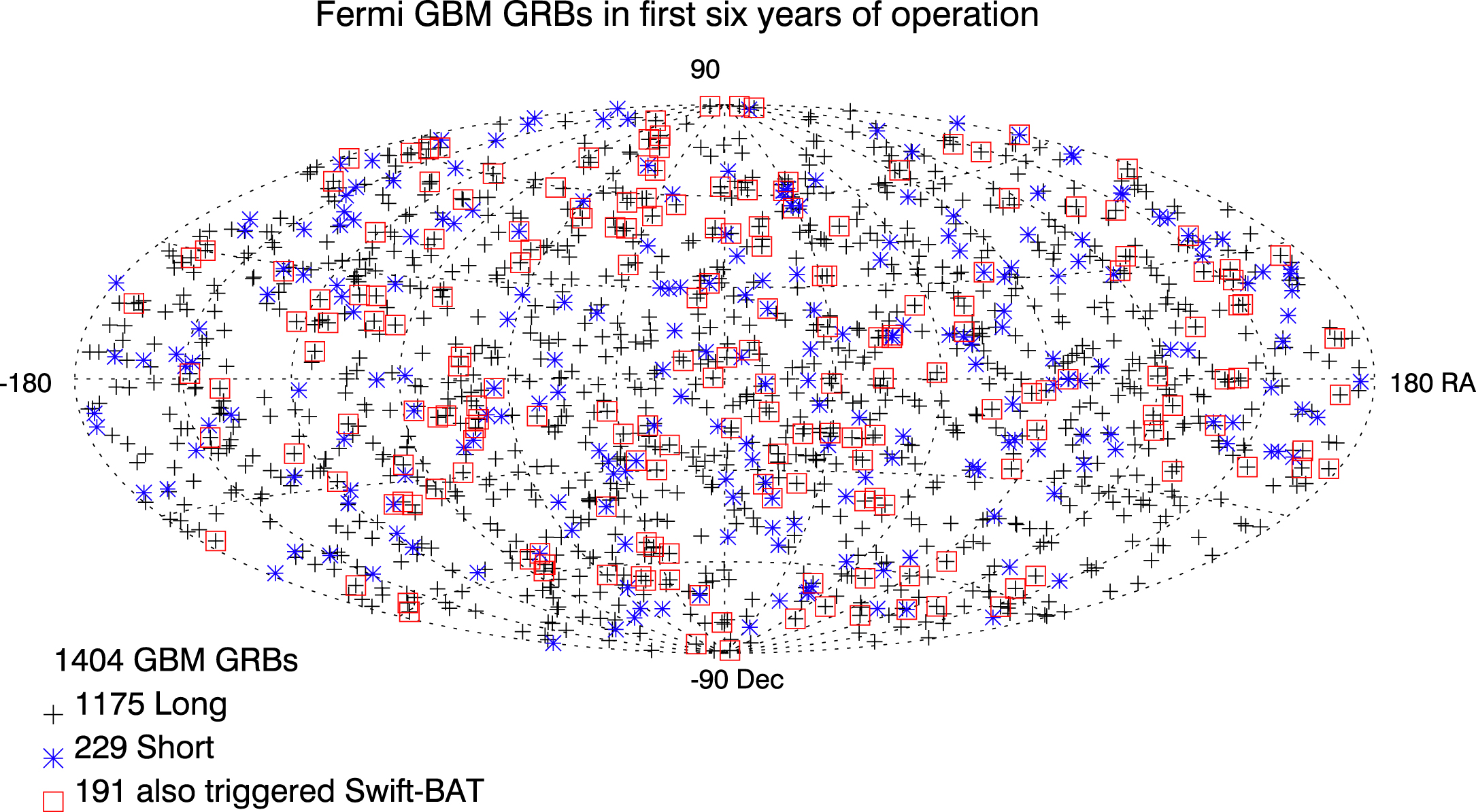
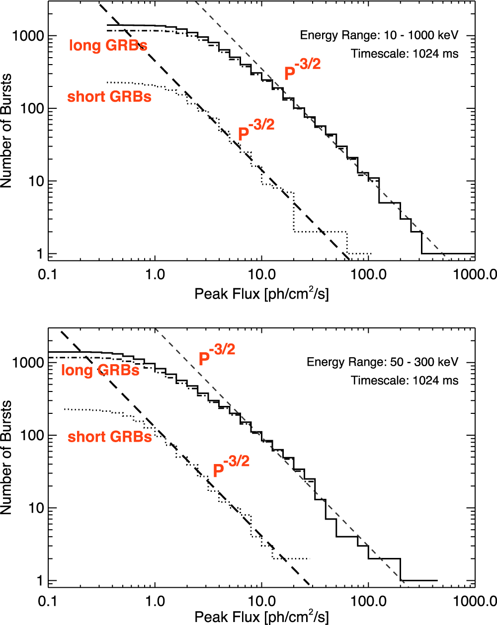
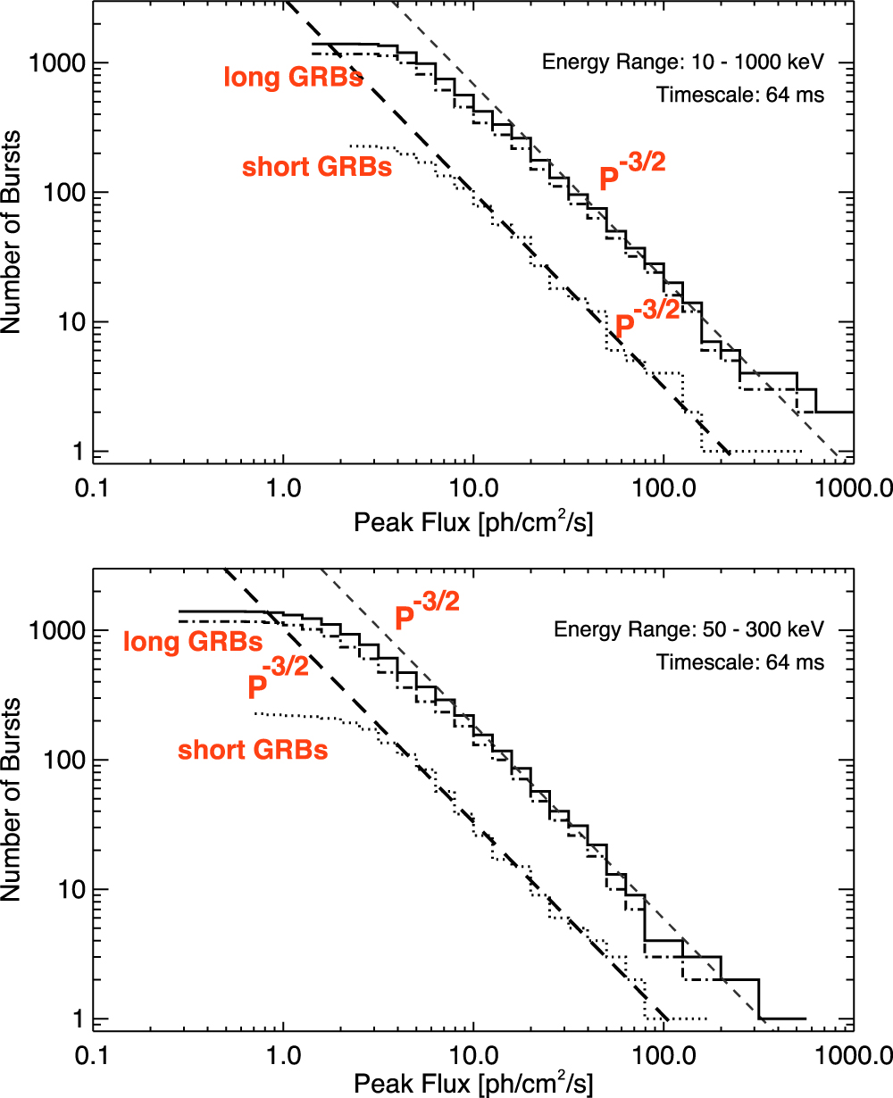
Figure 13. Integral distribution of GRB fluence (S ergs cm−2) in two energy ranges: 10–1000 keV (upper plot) and 50–300 keV (lower plot). Distributions are shown for the total sample (solid histogram), short GRBs (dots), and long GRBs (dashed–dotted), using T90 = 2 s as the distinguishing criterion. In each plot, a power law with a slope of −3/2 (dashed line) is drawn to guide the eye.
Download figure:
Standard image High-resolution image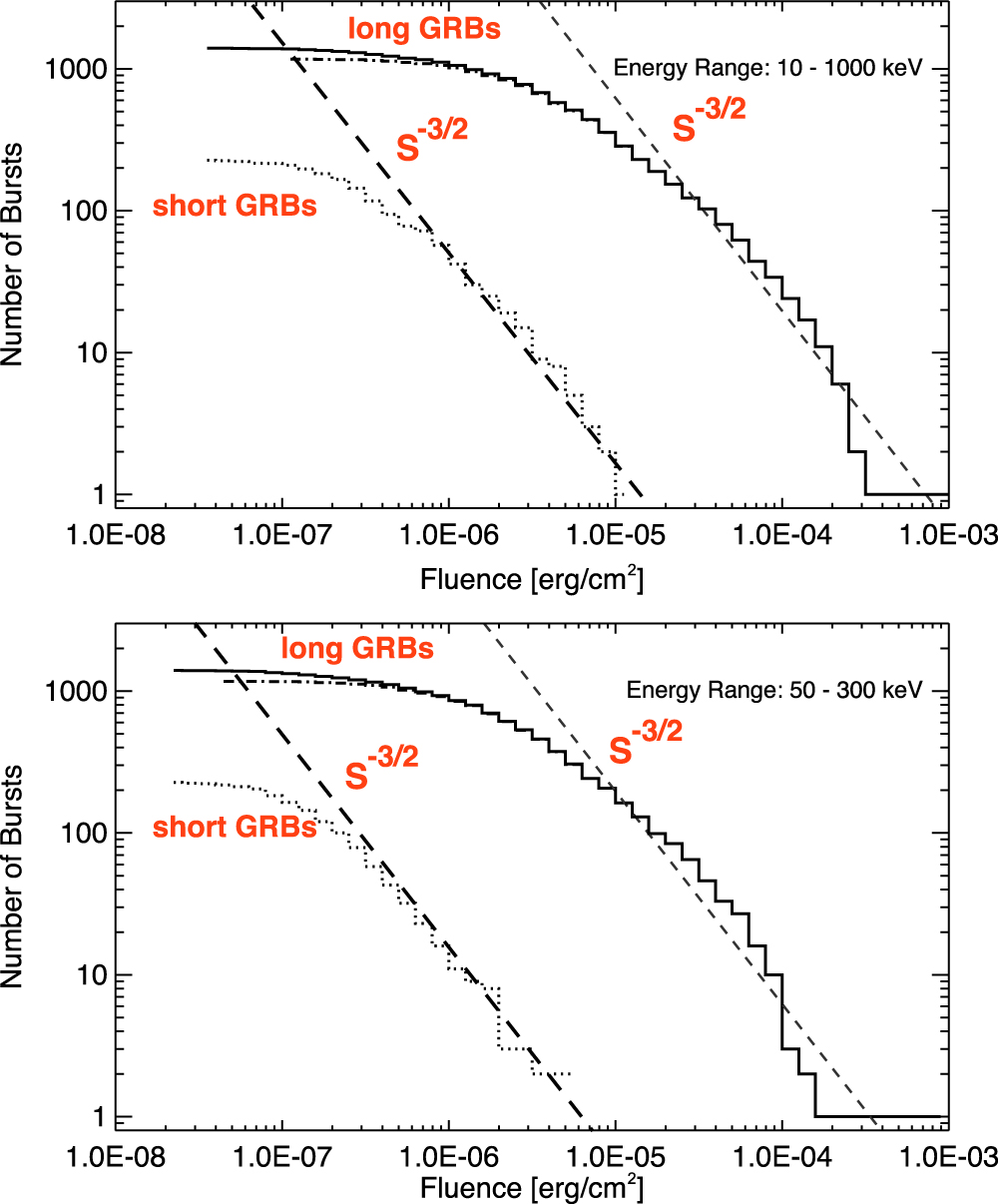
6. SUMMARY
The third GBM catalog comprises a list of 1403 cosmic GRBs that triggered GBM between 2008 July 12 and 2014 July 11. The increased sample of GRBs in this catalog confirms the conclusions of the earlier two year and four year catalogs. The six year average GRB rate detected by GBM is (0.662 ± 0.018) per day. The shortest and longest time interval between consecutive GRB triggers is 10 minutes and 11.77 days (with no interruptions), respectively. The shortest time interval is close to the minimum time for GBM to re-trigger. The longest time interval is ∼8 times larger than the average value of 1.5 days. Assuming that the GRB triggers follow Poisson statistics, this implies that such a large time gap could occur once in ∼10 years. The average rate of burst detections per year is (∼242 ± 6.5 year−1), which is only slightly smaller compared to the detection rate of the BATSE instrument of ∼300 year−1 (Paciesas et al. 1999). One would have expected a larger difference due to the superior detection sensitivity of BATSE. This perhaps can be explained by GBM's additional range of trigger timescales (primarily the 2 and 4 s timescales), which are compensating for the higher burst detection threshold of GBM (∼ 0.7 versus ∼ 0.2 photons cm−2 s−1 for BATSE). The distribution of GBM durations is consistent with the well-known bimodal distribution measured previously (Kouveliotou et al. 1993).This is supported by two independent analyses. Assuming a T90 value of 2 s to distinguish between short and long GRBs, the median durations of the two groups are 0.58 s and 26.62 s for the GBM sample, while they are 0.45 s and 30.75 s, respectively, for the BATSE sample. The median duration of GBM-detected long bursts is lower than that of BATSE-detected long GRBs. However, the fraction of short GRBs in the GBM sample is about 21%, which is not significantly different from that detected by BATSE, which is 24%.
Support for the German contribution to G.B.M. was provided by the Bundesministerium für Bildung und Forschung (BMBF) via the Deutsches Zentrum für Luft und Raumfahrt (DLR) under contract number 50 QV 0301. A.v.K. was supported by the Bundesministeriums für Wirtschaft und Technologie (BMWi) through DLR grant 50 OG 1101. S.M.B. and O.J.R. acknowledge support from Science Foundation Ireland under grant No. 12/IP/1288. H.F.Y. acknowledges support by the DFG cluster of excellence "Origin and Structure of the universe." A.G. is funded by the NASA Postdoctoral Program through Oak Ridge Associated Universities. The UAH co-authors gratefully acknowledge NASA funding from co-operative agreement NNM11AA01A. C.K. and C.A.W.H. gratefully acknowledge NASA funding through the Fermi GBM project.
Footnotes
- 19
- 20
GBM 8 Year Spectroscopy Catalog, in preparation.
- 21
γ-rays of energy >1 MeV will be registered in the overflow channel of the [Nai[Tl)] spectrum which have 10 times larger deadtime.
- 22
A table summarizing the intervals of the non-nominal trigger settings is posted at: http://fermi.gsfc.nasa.gov/ssc/data/access/gbm/llt_settings.html.
- 23
- 24
We used the spectral analysis package RMFIT, which was originally developed for time-resolved analysis of BATSE GRB data but has been adapted for GBM and other instruments with suitable FITS data formats. The software is available at the Fermi Science Support Center: http://fermi.gsfc.nasa.gov/ssc/data/analysis/user/. A tutorial is also available at http://fermi.gsfc.nasa.gov/ssc/data/analysis/scitools/rmfit_tutorial.html.
- 25
- 26
For GBM-derived locations, the statistical 1σ error is given. The GBM errors are not symmetric and the given value is the average of the error ellipse.
- 27
This information was drawn from the GCN archive, accessible at http://gcn.gsfc.nasa.gov/gcn3_archive.html. A more complete list of detections is available at http://www.ssl.berkeley.edu/ipn3/masterli.txt.
- 28
- 29
It may be noted that there were also times when BATSE triggers did not use the same threshold for all three timescales (see Table 1 in Paciesas et al. 1999). See http://heasarc.gsfc.nasa.gov/W3Browse/all/batsegrb.html.
- 30
Note that these are NOT the same as weighted means of log(HR).
- 31
PHEBUS was a Soviet–French gamma-ray burst experiment on board the GRANAT satellite launched before CGRO.