


ABSTRACT
We present an analysis of physical conditions in the Orion Veil, an atomic photon-dominated region (PDR) that lies just in front (≈2 pc) of the Trapezium stars of Orion. This region offers an unusual opportunity to study the properties of PDRs, including the magnetic field. We have obtained 21 cm H i and 18 cm (1665 and 1667 MHz) OH Zeeman effect data that yield images of the line-of-sight magnetic field strength Blos in atomic and molecular regions of the Veil. We find Blos ≈ −50 to −75 μG in the atomic gas across much of the Veil (25'' resolution) and Blos ≈ −350 μG at one position in the molecular gas (40'' resolution). The Veil has two principal H i velocity components. Magnetic and kinematical data suggest a close connection between these components. They may represent gas on either side of a shock wave preceding a weak-D ionization front. Magnetic fields in the Veil H i components are 3–5 times stronger than they are elsewhere in the interstellar medium where N(H) and n(H) are comparable. The H i components are magnetically subcritical (magnetically dominated), like the cold neutral medium, although they are about 1 dex denser. Comparatively strong fields in the Veil H i components may have resulted from low-turbulence conditions in the diffuse gas that gave rise to OMC-1. Strong fields may also be related to magnetostatic equilibrium that has developed in the Veil since star formation. We also consider the location of the Orion-S molecular core, proposing a location behind the main Orion H+ region.
Export citation and abstract BibTeX RIS
1. INTRODUCTION
Early-type stars irradiate their environments, creating photon-dominated regions (PDRs) with layers of ionized, atomic, and molecular gas. This interaction between stars and the surrounding interstellar medium (ISM), in turn, profoundly affects the evolution of the region, triggering further star formation or else quenching that process by dissipating the clouds. The nearest locale in which these interactions can be studied is the Orion Nebula neighborhood (436 ± 20 pc; O'Dell & Henney 2008). In this region, there are three PDRs viewed from distinctly different perspectives. One PDR is the Orion Nebula itself (NGC 1976, M42) and the molecular cloud OMC-1 that lies behind it. This region, viewed face-on and lying behind the Trapezium Cluster, can be studied in optical, infrared, and radio emission lines (e.g., Baldwin et al. 1991). The second Orion PDR is the Bright Bar. This region of bright optical emission along the southeast edge of the Orion Nebula is a PDR viewed nearly edge-on (e.g., Tielens et al. 1993; Hollenbach & Tielens 1997). Finally, the Orion Veil is a PDR viewed face-on, like the Orion Nebula; however, it lies in front of the Trapezium Cluster. Therefore, the Veil can be studied in optical and UV absorption lines against the Trapezium stars and in radio absorption lines against the nebular free–free emission. Abel et al. (2004) provide a simplified diagram of the Orion region, viewed sideways. O'Dell et al. (2009) provide a more detailed diagram, as do van der Werf et al. (2013, hereafter, vdWGO13). O'Dell (2001) and Ferland (2001) have reviewed observational data regarding the Orion Nebula and its environment.
Although the Veil contains a very small fraction of the mass of the Orion region, it offers an important laboratory for study of interstellar material associated with star formation. This importance comes from a rich body of observational data. These data include UV absorption lines from H2 and from various atomic species (see Abel et al. 2004, 2006, 2016), optical Ca ii and Na i absorption lines (O'Dell et al. 1993; Price et al. 2001), and radio absorption lines of 21 cm H i (e.g., vdWGO13) and 18 cm OH (this work). Abel et al. (2004, 2006, 2016) used observations of radio and UV absorption lines and spectral synthesis modeling to derive physical properties of the Veil such as temperature, density, and distance from the Trapezium stars.
In this study, we focus on the magnetic field of the Veil. The H i and OH lines are sensitive to the Zeeman effect in the atomic and molecular gas, respectively. Therefore, they offer an opportunity to image line-of-sight magnetic field strengths Blos across the Veil via aperture synthesis techniques. Zeeman effect studies of the Veil go back to the early work of Verschuur (1969) and Brooks et al. (1971), both of whom detected the H i Zeeman effect with single dishes. Later, Troland et al. (1989) used the Very Large Array (VLA) to image the magnetic field in the Veil via the H i Zeeman effect. Troland et al. (1986) detected the 1667 MHz OH Zeeman effect with a single dish. The present VLA data provide higher H i sensitivity and spatial resolution than those of Troland et al. (1989), and they add Zeeman effect data for the 1665 and 1667 MHz OH lines.
To orient the reader, we cite several published images of the Orion region. The first is the spectacular Hubble Space Telescope (HST) based optical image from Henney et al. (2007), reproduced here with modifications as Figure 1(a). For clarity, we add star symbols to the figure to identify the four Trapezium stars (see the figure caption for the meanings of other annotations). Most of the features of the Orion region discussed in this study are apparent in Figure 1(a). The names of the features are in general use; see O'Dell et al. (2009) and O'Dell & Harris (2010). The Huygens region is the brightest part of the Orion Nebula; it is about 6' (0.8 pc) across, and it appears in light colors centered on the Trapezium stars. The Bright Bar (see above) is a 3' long linear feature marking the southeast edge of the Huygens region. M43 is the small H+ region located about 8' north northeast of the Trapezium stars at the very top of Figure 1(a). M43 is excited by NU Ori, a B0-type star (Smith et al. 2005). The northeast Dark Lane is the area of obvious extinction that separates M43 from the Huygens region. The Dark Bay is another region of obvious extinction that extends like a finger across the Huygens region from east to west, terminating about 1' northeast of the Trapezium stars. Finally, Orion-S is a dense molecular core discussed in several sections below. Orion-S is not visible in Figure 1(a); however, the yellow circle centered about 1 5 southwest of the Trapezium stars denotes its location. Other notable Orion images are the 20 cm radio continuum and the HST Hα images of the Huygens region presented on the same scale by O'Dell & Yusef-Zadeh (2000). Comparison of these two images provides a sense of the optical extinction across the nebula, and O'Dell & Yusef-Zadeh use the images to construct an optical extinction image. They argue that optical extinction in this image comes principally from the Veil rather than from the main Orion H+ region. In Figure 1(b) we present a finder chart for individual positions where we consider H i data (smaller circles) and OH data (larger circles).
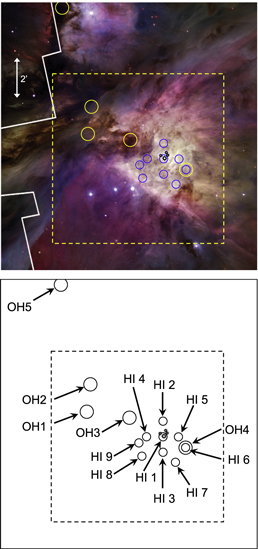
Figure 1. (a) Optical image of H+ regions M42 (center) and M43 (near top) taken from Henney et al. (2007). The Trapezium stars are denoted by black symbols; the largest symbol represents Theta 1C Ori. The vertical arrow is 2' (0.25 pc) long. Blue circles denote representative positions HI1–HI9 where unsaturated H i data were extracted (Table 4); the circles are 25'' in diameter, corresponding to the 21 cm synthesized beamwidth. Yellow circles denote representative positions OH1–OH5 where OH data were extracted (Table 3, Figures 2 and 3); the circles are 40'' in diameter, corresponding to the 1665 and 1667 MHz synthesized beamwidth. The dashed yellow rectangle indicates the field of view in Figures 5 and 6. (b) Finder chart for positions shown in Figures 1(a), 2, 5, and 6 and listed in Tables 3 and 4. The outer solid rectangle indicates the full field of view of Figure 1(a). The inner dashed rectangle indicates the field of view in Figures 5 and 6; it is the same as the dashed yellow rectangle of Figure 1(a).
Download figure:
Standard image High-resolution image2. OBSERVATIONS AND DATA ANALYSIS
Observations of the Zeeman effect in the 21 cm H i line and in the 18 cm OH main lines (1665 and 1667 MHz) were conducted with the NRAO Karl G. Jansky Very Large Array, (VLA).6 H i data were obtained in the VLA C-array, while OH data were obtained in the D array. All lines were observed in absorption against the Orion Nebula radio continuum. Observational parameters are given in Tables 1 and 2 for the H i data and the OH data, respectively. The general techniques for H i and OH Zeeman observations and data analysis with the VLA have been described by previous authors (e.g., Roberts et al. 1993, 1995; Sarma et al. 2000, 2013; Brogan & Troland 2001). Nonetheless, for the sake of completeness, we review these techniques below. We note that all published VLA Zeeman observations, as well as those described here, were made prior to the VLA upgrade that led to the JVLA designation in 2012. As is conventional for galactic VLA observations, velocities cited in this work are in the kinematic LSR (LSRK) reference frame; heliocentric velocities toward Orion are 18.1 km s−1 more positive than LSRK velocities. Henceforth, we refer to the LSRK reference frame as the LSR frame.
Table 1. Observational Parameters of 21 cm VLA H i Observations of the Orion A (M42) Region
| Parameter | Value |
|---|---|
| Frequency | 1420.4 MHz |
| Observing dates (project code, configuration) | 1991 Jan 20, Jan 21 (AT113, C) |
| Total observing time on source | 10.1 hr |
| Primary beam HPBW | 30' |
| Synthesized beam HPBW | 25'' × 25'' |
| Phase and pointing center (J2000) | 05h35m17 5, −05°23'37'' 5, −05°23'37'' |
| Primary flux density calibrator | 3C48 |
| Phase calibrator | 0607–085 (J2000) |
| Frequency channels per polarization | 128 (Two IF mode) |
| Total bandwidth | 195.3 kHz (41.2 km s−1) |
| Velocity coverage (LSR) | −17 to +24 km s−1 |
| Channel separation | 1.53 kHz (0.32 km s−1) |
| Channel resolutiona | 1.83 kHz (0.39 km s−1) |
| Pixel size in images | 4'' × 4'' |
| rms noise in line channels | 8.5 mJy beam−1 |
| rms noise in continuum | 16 mJy beam−1 |
| Sν to Tb | 1 mJy beam−1 = 1.1 K |
| Angular to linear scaleb | 1' = 0.13 pc |
Notes.
aAfter Hanning smoothing. bAssumes distance of 436 pc.Download table as: ASCIITypeset image
Table 2. Observational Parameters of 18 cm VLA OH Observations of the Orion A (M42) Region
| Parameter | Value |
|---|---|
| Frequencies | 1665.4 and 1667.4 MHz |
| Observing date (project code, configuration) | 1997 Nov 20 (AT209, D) |
| Total observing time on source | 5.9 hr |
| Primary beam HPBW | 26' |
| Synthesized beam HPBW | 47'' × 39'', PA = −23° |
| Phase and pointing center (J2000) | 05h35m175, −05°23'37'' |
| Primary flux density calibrators | 3C48, 3C147 |
| Phase calibrator | 0503+020 (J2000) |
| Frequency channels per polarization | 128 (Four IF Mode) |
| Total bandwidth | 195.3 kHz (35.2 km s−1) |
| Velocity coverage (LSR) | −12 to +24 km s−1 |
| Channel separation | 1.53 kHz (0.27 km s−1) |
| Channel resolution | 1.83 kHz (0.33 km s−1) |
| Pixel size in images | 10'' × 10'' |
| rms noise in line channels | 4.3 mJy beam−1 |
| rms noise in continuum | 9 mJy beam−1 |
| Sν to Tb | 1 mJy beam−1 = 0.27 K |
| Angular to linear scalea | 1' = 0.13 pc |
Note.
aAssumes distance of 436 pc.Download table as: ASCIITypeset image
We begin with an explicit statement of polarization definitions used in this work. We use the IEEE standards for sense of circular polarization. That is, in right circular polarization (RCP) the electric vector rotates clockwise as a wave propagates away from the observer. We also use the IEEE definition of Stokes parameter V = RHC − LHC. With these definitions, a magnetic field directed away from the observer generates a Zeeman effect in which the line observed in LCH is higher in frequency than the line in RCP. Such fields are defined as positive in sign. All fields observed in the Orion Veil are negative, that is, directed toward the observer.
VLA Zeeman observations at 18 and 21 cm were made with dual native circular polarization receivers (RHC and LHC) on each telescope. Therefore, the construction of Stokes V profiles, necessary for detection of the Zeeman effect, requires subtraction of data from two independent receiver/IF systems with different bandpass shapes. The subtraction process introduces an instrumental bandpass shape into the Stokes V profiles. To mitigate this effect, we switched the RF transfer switches on each telescope every 10 minutes. This step inverts the senses of circular polarization sent to the two IF systems. When data from both switch positions are combined, bandpass differences downstream from the switches are eliminated. H i observations were made in the Two IF Mode of the original VLA correlator (one spectral line, two circular polarizations). OH observations were made in the Four IF Mode (two spectral lines, two circular polarizations). Finally, calibration sources for the H i observations were observed at frequencies displaced above and below the H i line by 1 MHz (210 km s−1). Phase calibration solutions were then determined from the average of calibration scans at both displaced frequencies. This procedure ensured that galactic H i emission did not affect calibration source data.
Calibration and imaging of the H i and OH data were done with the NRAO AIPS package. Standard techniques were applied to calibrate RHC and LHC uv data from each transfer switch position (i.e., four data sets independently calibrated for each spectral line). Further AIPS analysis led to the production of Stokes I, Stokes V, and optical depth image cubes for the H i line and for the two OH lines. In addition, we took special steps to remove maser emission from the OH data, as described below. These steps were taken to prevent images of the Stokes I and V OH thermal lines from being dominated (and dynamic range limited) by the strong maser lines. Note that errors in absolute calibration of the data do not affect Zeeman measurements since magnetic field strengths are derived from ratios involving Stokes I and V. However, the absolute VLA flux density scale is expected to be accurate to about 5%.
We used the AIPS task IMAGR to create Stokes I and Stokes V image cubes. For the H i line, we created cleaned Stokes I image cubes from bandpass-corrected, continuum-subtracted uv data. We chose a robustness of 1, intermediate between uniform and natural weighting of the uv data. This choice was a compromise between the conflicting needs to achieve high angular resolution and low noise. The H i Stokes V image cubes were created by IMAGR from uv data that had not been bandpass corrected. With the transfer switching technique described above, the Stokes V bandpasses were acceptable without correction. Moreover, bandpass correction adds noise to the Stokes V data, reducing sensitivity to the Zeeman effect. Note that IMAGR calculates Stokes I/2 and Stokes V/2 images.
For each of the OH lines, we removed maser emission from the uv data cubes via a multistep process. We applied this process only to the maser channels, that is, channels with significant maser emission. First, we created all-channel, bandpass-corrected, continuum-subtracted image cubes in RCP and LCP. For each image cube, we performed self-calibration on the maser channels and reimaged each such channel. Next, we identified clean components in these channel images by specifying small clean boxes around each maser position. Then we subtracted the contributions of the maser clean components from the uv data via UVSUB and reimaged the maser channels in RCP and LCP. Finally, we replaced the original maser channels in the RCP and LCP image cubes with the newly maser-free maser channels. Sarma et al. (2000) applied the same techniques to remove the effects of OH masers in NGC 6334. To generate optical depth image cubes for H i and OH lines, we used task COMB to combine the continuum-subtracted and cleaned Stokes I cube with a cleaned continuum map constructed from line-free channels in the Stokes I profiles. We were careful to clean the Stokes I cube and the continuum image in consistent ways to mitigate systematic errors in the optical depth calculations.
Once the Stokes I and V image cubes were produced for each line with AIPS tasks, we undertook the Zeeman analysis using the Multichannel Image Reconstruction, Image Analysis and Display (MIRIAD) package with task ZEEMAP. This task performs a pixel-by-pixel fit of the Stokes V profile to the derivative of the Stokes I profile. The fitting process, most recently described by Sarma et al. (2013), yields estimates of the line-of-sight magnetic field strength Blos (and its sign), together with the error σ(Blos). The fit for each pixel can be done over a specified range of spectral channels. For the Orion H i data, we performed independent fits over two ranges of channels to estimate Blos and σ(Blos) for each of two velocity components in the Veil (Section 3.2). As is customary in imaging VLA data, the pixel separations were chosen to be smaller than the synthesized beamwidths (see Tables 1 and 2). Therefore, values for Blos and its error derived for adjacent pixels are not independent. Rather, these values are averages over a synthesized beam centered on a particular pixel.
3. RESULTS
3.1. Radio Continuum
H i and OH absorption lines are observed against the radio free–free continuum of M42 and M43. An image of this continuum, derived by combining information from line-free channels in the Stokes I image cube, is a natural product of the data. Our 21 cm continuum image has a synthesized beamwidth of 25'' (0.05 pc); our 18 cm (1665 and 1667 MHz) OH images have a synthesized beamwidth of 40'' (0.09 pc). The peak brightness of our 21 cm image is 4.7 Jy beam−1, equivalent to brightness temperature TB = 5100 K. We do not present our continuum images as separate figures. Equivalent or higher spatial resolution Orion continuum images at similar wavelengths are available in the literature. See especially the 21 cm continuum image of vdWGO13. See also the 20 cm image of O'Dell & Yusef-Zadeh (2000) and the wide-field 330 MHz (90 cm) image of Subrahmanyan et al. (2001). We recover a total 21 cm continuum flux of 290 ± 15 Jy for M42. This value is to be compared with 335 ± 15 Jy found for M42 by vdWGO13. M43 contributes an additional 12 ± 2 Jy to our data, compared to 14 ± 2 Jy for vdWGO13. Errors reflect uncertainties in the allocation of flux between M42 and M43. See van der Werf & Goss (1989, hereafter vdWG89) and vdWGO13 for additional information about the total Orion 21 cm continuum flux density.
3.2. H i Optical Depths
We constructed an H i optical depth image cube from the Stokes I image cube and the Stokes I continuum image. Toward the brightest part of M42, we measure peak H i optical depths as high as τ0, H i ≈ 5. Over much of the Huygens region, we measure τ0,H i of up to 4, and we measure H i optical depths out to the continuum brightness contour that is 3% of the peak. In general, H i optical depths increase from the southwest toward the northeast of the Veil, and the H i lines are saturated in the northeast sector of the image. Line saturation precludes measurement of τH i ∝ N(H0)/Tex, where Tex is the H i line excitation temperature. However, line saturation does not preclude detection of the H i Zeeman effect; see Section 3.4.
The spatial variation of H i optical depths has already been described by other authors beginning with Lockhart & Goss (1978). In particular, vdWG89 observed H i absorption in the Veil with the VLA C-array. Although their velocity resolution was half that of the present observations, they were able to identify several velocity components. Principal among them are components A and B (their designations, adopted here). Components A and B have typical LSR center velocities of 5.0 and 1.3 km s−1, respectively, and typical FWHM of 2.5 and 3.6 km s−1, respectively (Table 4). Clearly, there are multiple layers of H0 gas in the Veil. vdWG89 performed a Gaussian analysis of their H i optical depth data cube. From this analysis, they derived images of N(H0)/Tex across the Veil for each component separately. They found that components A and B exist across the entire radio continuum source (M42 and M43), with peak optical depths generally higher in component A. However, an inspection of our more sensitive and higher velocity resolution H i optical depth profiles clearly reveals that the kinematical structure of the Veil is too complicated to be fully described by a two-component model. Nonetheless, the Gaussian decomposition done by vdWG89 provides a good qualitative idea of the distribution of H i velocity components A and B for which we have H i Zeeman effect images (Section 3.4). vdWGO13 also present extensive VLA data on H i absorption and emission in the Veil. However, these authors concentrate on small-scale structure, generally at velocities outside the range occupied by components A and B.
3.3. OH Optical Depths and Column Densities
The OH optical depth cubes show that OH absorption across the Veil is qualitatively different from H i absorption in two ways. For one, OH absorption is only detected in four isolated regions, not across the entire Veil. The second difference is that the OH profiles usually consist of a single velocity component, compared to at least two components in the H i profiles. OH absorption is not detected toward the Trapezium Cluster. This absence is expected, given the very low H2 abundance toward the Trapezium stars (N(H2)/N(H0) ≈ 10−6.5) measured by UV absorption lines (Abel et al. 2016). The Veil along this line of sight is almost completely atomic owing to the very high stellar radiation field from the Trapezium.
Four regions of OH absorption appear in Figure 2. Here we present a color-coded image of the velocity-integrated 1667 MHz OH optical depth, in units of [N(OH)/Tex] × 1014 cm−2 K−1, where Tex is the 1667 MHz excitation temperature. To calculate N(OH)/Tex from the velocity-integrated optical depth profiles, we use the conversion factor given in Roberts et al. (1995), C1667 = 2.28 × 1014 cm−2 K−1 (km s−1)−1. This factor assumes LTE conditions. For reference, we overlay 1667 MHz continuum contours in the figure. These contours clearly show M42, as well as M43 to the northeast. Also note the circles in Figure 2 denoting five representative positions in the OH data discussed in the next paragraph. These five circles are also shown in the finder chart of Figure 1(b) (larger circles). The four OH absorption regions are as follows: (1) The most prominent absorption is toward the northeast Dark Lane along the northeast edge of M42. Here, peak 1667 MHz optical depths reach τ0,1667 ≈ 1, perhaps higher in regions of saturation. (2) Much weaker OH absorption exists toward the Dark Bay. This absorption appears in Figure 2 as a tongue extending westward from the northeast Dark Lane toward the brightest region of radio continuum emission. OH optical depths are highest (τ0,1667 ≈ 0.04) in the direction of Knot 1 identified by O'Dell & Yusef-Zadeh (2000) in their optical extinction image. (3) OH absorption (τ0,1667 ≈ 0.12) is observed approximately 1' to the southwest of the peak continuum brightness. This direction closely coincides with the Orion-S molecular core (e.g., Henney et al. 2007), and the absorption appears as a distinct, nearly circular region, suggesting that it is barely resolved in the VLA data. We refer to this absorption as the Orion-S OH absorption, although the connection between OH and Orion-S bears further consideration. See Section 4.4. The Orion-S OH absorption feature has a clear counterpart in H i absorption, with peak optical depth τ0,H i ≈ 0.2 in the present data and 0.45 in the higher spatial resolution data of vdWGO13. See Section 4.4 and Figure 10. Finally, (4) strong OH absorption (τ0,1667 ≈ 0.6) appears along the eastern edge of M43. This absorption is clearly associated with the dark filament of optically obscuring material in Figure 1(a). This same filament is visible in the 800 μm OMC-1 dust continuum image of Johnstone & Bally (1999).
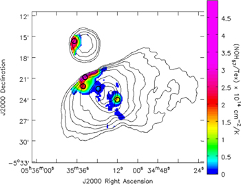
Figure 2. Color: integrated 1667 MHz OH optical depth in units of [N(OH)/Tex] × 1014 cm−2 K−1, where Tex is the excitation temperature. Black contours represent the 1667 MHz continuum brightness; isolated contours in the northeast sector of the image are for M43. Synthesized beam size is 40''. Black circles are 40'' in diameter; they denote positions OH1–OH5, for which OH 1667 MHz optical depth profiles are shown in Figure 3 and positions and other data are given in Table 3. Also, see the finder chart in Figure 1(b).
Download figure:
Standard image High-resolution imageTo illustrate the nature of OH absorption toward Orion, we choose five representative positions in our image data. We label these positions OH1–OH5. Two of these positions are located in the northeast Dark Lane, and one is located in each of the Dark Bay, Orion-S, and M43 regions. The locations of these five positions are shown in Figures 1(a), 1(b), and 2 as circles of 40'' diameter, the 1665 and 1667 MHz synthesized beamwidth. Table 3 lists these positions and their relevant parameters; Table 2 lists the channel separation and resolution. Figure 3 shows 1667 MHz OH optical depth profiles for each position. Note that the optical depth profile for Orion-S is about a factor of two wider than any of the other profiles. Comparison of the OH optical depth profiles with H i optical depth profiles at these five positions (the latter not shown) indicates that the OH lines always lie within the velocity range of the saturated H i lines. Except for the Orion-S position (Figure 10), it is not possible to identify OH lines with specific H i velocity components owing to H i line saturation.

Figure 3. 1667 MHz OH optical depth profiles for positions OH1–OH5 listed in Table 3 and shown as yellow circles in Figure 1(a), larger black circles in Figure 1(b), and black circles in Figure 2. Synthesized beamwidth is 40''; channel separation is 0.27 km s−1.
Download figure:
Standard image High-resolution imageTable 3. Parameters for Positions with 18 cm OH Absorption toward Orion A
| No. | Position Location | R.A.a | Decl.a | Vo,67b | ΔV67c | τo,67d | τo,67/τo,65e | N(OH)f | Avg | N(H)h |
|---|---|---|---|---|---|---|---|---|---|---|
| (J2000) | (J2000) | (km s−1) | (km s−1) | (cm−2) | (mag) | (cm−2) | ||||
| OH1 | Northeast Dark Lane 1 | 05h35m322 |
−05°22'06'' | 6.4 | 2.7 | 0.37 | 1.7 | 4.7 × 10¹⁵ | 58 | 1.5 × 10²³ |
| OH2 | Northeast Dark Lane 2 | 05h35m314 |
−05°20'46'' | 6.6 | 1.9 | 0.97 | 2.2 | 8.8 × 10¹⁵ | 110 | 2.7 × 10²³ |
| OH3 | Dark Bay | 05h35m234 |
−05°22'29'' | 3.7 | 2.7 | 0.04 | 1.9 | 5.6 × 10¹⁴ | 7 | 1.7 × 10²² |
| OH4 | Orion-S | 05h35m121 |
−05°23'56'' | 6.9 | 5.2 | 0.12 | 1.2 | 3.8 × 10¹⁵ | 48 | 1.2 × 10²³ |
| OH5 | M43 | 05h35m377 |
−05°15'46'' | 9.6 | 2.2 | 0.59 | 1.9 | 5.8 × 10¹⁵ | 72 | 1.8 × 10²³ |
Notes.
aPosition of the center of the 40'' synthesized beam at 18 cm. bCenter velocity of the 1667 MHz OH line. cFWHM width of the 1667 MHz OH line. dPeak optical depth of the 1667 MHz OH line. eRatio of peak optical depths of the 1667 and 1665 MHz OH lines. The LTE value is 1.8. fOH column density, taken as the average of OH column densities computed separately from the 1665 and 1667 MHz OH lines. Calculation of OH column densities from the individual OH lines was done with the relationships of Roberts et al. (1995), assuming Tex = 20 K. gAv estimated from the ratio N(OH)/Av = 8 × 1013 cm−2 mag−1 of Crutcher (1979), who states that the ratio is valid over the range Av = 0.4–7 mag. If the ratio N(OH)/Av decreases for Av > 7 mag, owing to freeze-out or chemical conversion of OH to other species, then some values of Av in this column are underestimates. hN(H) estimated from the ratio Av/N(H) = 4 × 10⁻²² mag cm2 cited by Abel et al. (2004) for the Orion region. Some of these values could be underestimates; see note regarding Av immediately above.Download table as: ASCIITypeset image
For each of the five representative positions of OH absorption (Table 3), we derive N(OH) from the velocity-integrated 1665 and 1667 MHz optical depth profiles. To do so, we use the standard conversion factors C1665 and C1667 from Roberts et al. (1995, see above), and we assume Tex = 20 K for both OH lines. However, N(OH) ∝ Tex, and Tex cannot be measured from our absorption-line data. Tex can only be measured from a combination of absorption and emission lines along the same line of sight. Using such galactic data toward extragalactic continuum sources, Liszt & Lucas (1996) found Tex ≈ 4–13 K for the OH main line transitions. Recently, C. Heiles (2016, private communication) analyzed a similar but more extensive data set from the Millennium Survey (Heiles & Troland 2005). Heiles found Tex for the OH main lines in the range 2–15 K, with the majority of the values below 10 K and many less than 5 K. These OH data toward extragalactic continuum sources likely sample low-density molecular gas (n(H) ≈ 102–3 cm−3), where the OH lines are very subthermally excited (Tex ≪ TK). OH-bearing gas in the Veil is likely to be much denser (see note a to Table 6) and somewhat warmer, the latter owing to its proximity to the Trapezium. Therefore, we expect Tex to be higher in the Veil than in the low-density molecular gas. According to the theoretical study of Guibert et al. (1978), Tex for the OH main lines is rather insensitive to TK. However, Tex is sensitive to n(H). For a gas with TK = 50 K, Guibert et al. calculate that Tex increases from 5 K to an asymptotic value of 30 K in the range n(H) ≈ 102–104 cm−3 (see their Figure 2). Given this trend, we believe that our assumption of Tex = 20 K for the Veil OH lines is reasonable and likely to be correct to within a factor of two.
Having estimated N(OH) as described above, we use standard conversion factors to scale N(OH) to N(H) and to Av, where N(H) = N(H0) + 2 N(H2). Results are given in Table 3 along with the conversion factors we have used. Note that values of Av in Table 3 are not direct measures of optical extinction like those reported by O'Dell & Yusef-Zadeh (2000). Judging from Table 3, most of the OH absorption arises in high column density regions (Av > 50). The only exception is the Dark Bay, for which Av ≈ 7. Also, we note that the ratios of peak OH optical depths τ0,1667/τ0,1665 deviate from the LTE value of 1.8 for several of the positions in Table 3. Ratios greater than the LTE value indicate nonthermal excitation of the 18 cm OH levels, a common phenomenon (e.g., Crutcher 1977). Ratios less than the LTE value may also indicate nonthermal excitation and/or clumping of optically thick gas on scales smaller than the synthesized beamwidth.
3.4. The H i Zeeman Effect
A principal goal of these observations is to study the distribution of magnetic field strengths in the Veil. The strong radio continuum emission of the Orion H+ region leads to strong H i absorption lines, and, via the H i Zeeman effect, to measurements of Blos in the H0 layers of the Veil. Aperture synthesis data yield images of Blos across the Veil, and they do so independently for different velocity components. For the Veil data, we found evidence of the Zeeman effect in both velocity components A and B. Accordingly, we fitted separately over the channel ranges appropriate to component A (5.3–22 km s−1) and component B (−14.7 to 3.6 km s−1). Note that these velocity ranges include line-free channels necessary for the least-squares fits. We discuss below the images of Blos derived for these two components. We note that sensitivity to Blos is highly variable among pixels in the images. This variability arises from variations across the Veil in radio continuum brightness, line optical depth, and line width. Higher sensitivities to Blos arise in pixels where the radio continuum brightness and line optical depths are higher and where lines are narrower. Velocity component A has generally higher optical depths and narrower lines than component B. Therefore, the image of Blos for component A has better sensitivity over a larger number of pixels. In Figure 4, we show an example of 21 cm Stokes I/2 and V/2 profiles. These profiles are for a pixel in the images lying close to the center of the Trapezium. At this particular position, Blos is the same to about 1σ for the two velocity components. Table 1 lists the channel separation and resolution. The synthesized beamwidth is 25''.

Figure 4. Stokes I/2 and Stokes V/2 profiles toward the Trapezium stars (position HI1 in Table 4) for the 21 cm H i line. The dashed profiles overlaid on the Stokes V/2 profile are derivatives of the Stokes I/2 profiles, scaled separately for the best-fit values of Blos in H i components A and B, −52.4 ± 4.4 μG and −47.3 ± 3.6 μG, respectively. Velocities are LSR. Synthesized beamwidth is 25''; channel separation is 0.32 km s−1.
Download figure:
Standard image High-resolution image3.4.1. The H i Zeeman Effect in Component A
In Figure 5 we present an image of Blos in Veil H i velocity component A. Figure 5 (synthesized beamwidth 25'') is one of the most detailed images of interstellar magnetic field strengths published to date. Blos in component A is uniformly negative (magnetic field pointed toward the observer). For simplicity, we use the symbol Blos below to signify  . Also, Figure 5 has been masked to include only those pixels for which
  /σ(Blos) > 3. Perhaps the most striking characteristic of Figure 5 is the relative uniformity of Blos over much of the Veil, with most values in the range 30–60 μG. However, there is a tendency for Blos to increase gradually from southwest to northeast, roughly similar to the increase in H i optical depths of components A and B (see vdWG89). Also, there appears to be a ridge of enhanced Blos extending from the southwest diagonally across the Veil to the northeast and widening toward the northeast. In this ridge, Blos ≈ 50–60 μG, whereas on either side of the ridge Blos ≈ 30–40 μG. The ridge of enhanced Blos coincides approximately with a ridge of enhanced N(H0)/Tex in the image of component A presented by vdWG89. An indication of the ridge also appears in the H i optical depth image of vdWGO13 for a velocity of 8.4 km s−1, on the unsaturated red wing of H i component A. Finally, there are isolated regions of higher Blos in Figure 5, most obviously in the northeast sector of the source. Here, Blos is typically >100 μG, reaching 300 μG in one small region about 30'' in size. Other isolated regions of higher Blos (75–100 μG) lie in the northern part of the Veil and near the southwest edges of the image in Figure 5. Overall, the image of Blos for component A is consistent with the equivalent image in Troland et al. (1989), where component A is labeled the high-velocity (HV) component. However, the present results in Figure 5, with their higher sensitivity and spatial resolution (25'' versus 40''), include values of Blos for more independent pixels, and they reveal high field strengths (Blos > 100 μG) in the northeast sector of the Veil, a region not included in the earlier results of Troland et al.
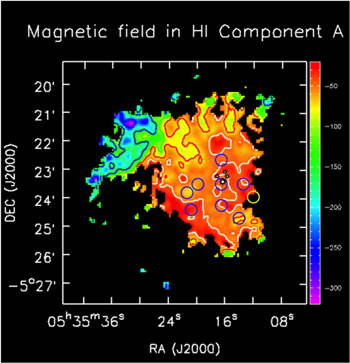
Figure 5. Image of Blos (colors and contours) for H i component A. Contours are at Blos = −45 μG (white), −75 μG (red), −100 μG (green), and −150 μG (blue). The image has been masked to include only those pixels for which  /σ(Blos) > 3. The Trapezium stars are denoted by black symbols as in Figure 1(a). Circles of 25'' diameter (synthesized beamwidth) denote positions HI1–HI9 in Table 4 for which values of Blos are given. For comparison purposes, the field of view of this image is shown in Figures 1(a) and (b) as dashed rectangles. Also, see the finder chart in Figure 1(b).
Download figure:
Standard image High-resolution image3.4.2. The H i Zeeman Effect in Component B
In Figure 6 we present an image of Blos in Veil H i velocity component B (synthesized beamwidth 25''). Again, we have masked the figure to include only pixels for which  /σ(Blos) > 3. As for component A, all values are negative, and we use the symbol Blos below to signify
  . Since component B is generally weaker and wider than component A, sensitivity to Blos is lower, and Figure 6 displays fewer values of Blos than Figure 5. Overall, the image of Blos for component B is remarkably similar to that for component A. In particular, Blos for component B is quite uniform over most of the image, with most values Blos ≈ 50–60 μG. Also, values for Blos in component B increase toward the northeast sector of the source, reaching 100 μG or more. This behavior, too, is similar to that for component A. In detail, however, there are differences in the distribution of Blos for the two H i velocity components. For example, a peak in Blos for component B in the southwest region of the image (90 μG) nearly coincides in position with a minimum in Blos for component A (30 μG). The image of Blos for component B is consistent with the equivalent image in Troland et al. (1989), where component B is labeled the low-velocity (LV) component. However, the earlier image of Blos for this component includes a very few independent measurements owing to severe sensitivity limitations.

Figure 6. Image of Blos (colors and contours) for H i component B. Same as Figure 5, except circles denote positions HI1–HI4 and HI7 in Table 4 for which values of Blos are given.
Download figure:
Standard image High-resolution image3.5. The OH Zeeman Effect
The present data provide the first aperture synthesis measurement of Blos in molecular regions of the Veil. Previously, Troland et al. (1986) detected the 1667 MHz OH Zeeman effect toward Orion A using the Nancay telescope. They found Blos,1667 = −125 ± 20 μG, positioning the Nancay 35 × 19' beam (FWHM, right ascension and declination, respectively) 3' east of the Orion A radio continuum peak (see contours in Figure 2). As for the H i data (Section 3.4), the OH data have highly variable sensitivities to the Zeeman effect. Careful examination of our 1667 MHz Stokes I and V profiles reveals the Zeeman effect reliably detected in only one independent position, OH1 in the northeast Dark Lane (Table 3). Here, Blos,1667 = −350 ± 47 μG and Blos,1665 = −151 ± 46 μG. At this same position, Blos,H i is −183 ± 32 μG in H i component A. In Figure 7 we present Stokes I/2 and V/2 profiles for the 1665 and 1667 MHz lines. The synthesized beamwidth is 40''; the channel separation is 0.27 km s−1. The center velocity of the lines in this figure coincides quite well with the center velocity of the lines observed by Troland et al. (1986) at Nancay. Evidently, these authors sampled with a single dish nearly the same region of the Veil as we did with the VLA. The higher spatial resolution of the VLA likely accounts for the higher field strength detected with the aperture synthesis instrument.
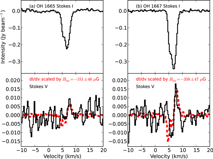
Figure 7. Stokes I/2 and Stokes V/2 profiles for the 1665 MHz OH line (left) and for the 1667 MHz line (right) at position OH1. The red dashed lines overlaid on the Stokes V/2 profiles are derivatives of the Stokes I/2 profiles, scaled separately for the best-fit values of Blos in the two OH lines. Velocities are LSR. Synthesized beamwidth is 40''; channel separation is 0.27 km s−1.
Download figure:
Standard image High-resolution imageValues of Blos derived from the 1665 and 1667 MHz lines only agree to within 2σ. Also, the 1665 MHz Stokes V/2 profile in Figure 7 shows scant signs of the Zeeman effect. The Orion field of view includes OH masers that we attempted to remove in the uv-plane (Section 2). These masers are much stronger in the 1665 MHz line, and their effect cannot be completely removed from the synthesis data. Therefore, we suspect that residual maser contamination is present in the 1665 MHz Stokes V/2 profile of Figure 7. Troland et al. (1986) noted the same phenomenon. Their single-dish 1665 MHz Stokes V profile shows clear evidence for maser contamination near the thermal OH absorption line velocity. Yet they find no such contamination in their 1667 MHz Stokes V profile. With these considerations in mind, we assume that our Zeeman effect result at 1667 MHz is more reliable than that at 1665 MHz, so we use the former result in our energy analysis of Section 4.2.
4. DISCUSSION
4.1. Morphological Connections among Blos, N(H0), and Optical Extinction
The present data allow for a comparison among images of different physical parameters across the Veil. These images include Blos in H i components A and B, N(H0)/Tex in components A and B, and optical extinction across the Veil. (For orientation purposes, recall that the dashed yellow rectangle in the optical image of Figure 1(a) corresponds to the fields of view of the Blos maps in Figures 5 and 6.) Comparisons among images are necessarily incomplete because images of the relevant parameters are incomplete over different parts of the Veil. For example, images of N(H0)/Tex only provide information in the southwest regions of the Veil, where the H i line is unsaturated. Images of Blos are limited by sensitivity to the Zeeman effect, they only cover the inner parts of the Veil (especially for H i component B), and the images are only sensitive to one component of the magnetic field. The optical extinction images, likewise, only cover the inner Veil, where O'Dell & Yusef-Zadeh (2000) could measure extinctions.
Despite the limitations in image coverage, we find morphological similarities between the distributions of N(H0)/Tex and magnetic fields across the Veil. In particular, there is a significant and previously established (vdWG89) tendency for the velocity-integrated N(H0)/Tex to increase from the southwest toward the northeast of the Veil. This trend also applies individually to H i components A and B. Likewise, there is a significant tendency for Blos in H i component A to increase in the same direction, becoming highest in the direction of the northeast Dark Lane, where the H i line is deeply saturated (Figure 5, Section 3.4). The image of Blos in H i component B (Figure 6) is more limited in coverage, so this same trend is not so obvious. Nonetheless, the highest values of Blos for component B also occur in the northeast region of the image, just as they do for component A. Considering the morphology in slightly more detail, both N(H0)/Tex in H i component A (vdWG89) and Blos in the same component display a ridge of higher values along a southwest to northeast axis. These morphological similarities between H i and Blos suggest a general tendency toward constant mass-to-flux ratio (∝ N(H0)/Blos) in the Veil. The similarities in morphology among N(H0)/Tex in components A and B and Blos in components A and B imply a very close association between these two components despite their difference in center velocities.
The morphology of the optical extinction image (O'Dell & Yusef-Zadeh 2000) bears a more complex relationship to the morphologies of the N(H0)/Tex and Blos images. As a result, it seems unlikely that the Dark Bay is directly associated with H i components A and B. Optical extinction increases from southwest to northeast across the image. Also, there is some indication of a ridge of enhanced extinction along this axis. This morphology is similar to those of Blos and N(H0)/Tex in components A and B (see above). Indeed, the morphological similarities between optical extinction and N(H0)/Tex across the Veil led O'Dell & Yusef-Zadeh (2000) to conclude that most of the optical extinction of the Orion Nebula arises in the H0 layers of the Veil rather than in the ionized gas itself. However, there is one obvious exception to these morphological similarities, the Dark Bay. No indication of the Dark Bay appears in the images of Blos (Figures 5 and 6). Therefore, it seems likely that the Dark Bay is physically separated from Veil H i components A and B. This suggestion is consistent with the morphology of optically obscuring material shown qualitatively in Figure 1(a). In this optical image, the Dark Bay appears to be a westward extension of very optically obscuring material to the east and northeast of the Orion Nebula. The optically obscuring material includes not only the Dark Bay but also the northeast Dark Lane and the filament of obscuring material partially covering M43. Perhaps this whole complex of optically obscuring material is a part of OMC-1 that lies in front of Veil H i components A and B.
Finally, we comment on the connection between OH absorption and the optical extinction image. OH absorption is only observed in four regions of the Veil (Section 3.3). Of these four regions, only two lie within the area covered by the optical extinction image of O'Dell & Yusef-Zadeh (2000). These regions are the Dark Bay and Orion-S, where Av in the optical extinction image is about 5.5 and 1.4 mag, respectively. There is no detectable OH absorption toward the Trapezium stars (Av ≈ 2). Also, there is no OH absorption toward the Southwest Cloud (SW Cloud in O'Dell & Yusef-Zadeh 2000) about 2' southwest of the Trapezium, where Av ≈ 3. The Southwest Cloud appears in Figure 1(a) as a distinct, scorpion-shaped patch of extinction near the southwest edge of the bright H+ region. If we exclude Orion-S from consideration, as a different environment (see Section 4.4), then OH absorption is only observed in the Veil when Av > 5. The absence of OH absorption except at relatively high Av is not surprising since OH requires significant shielding to survive in an environment of such intense stellar radiation. This statement is consistent with the Cloudy spectral synthesis code model of Orion-S (O'Dell et al. 2009). In this model, significant OH does not form until Av reaches about 4 mag. Although physical conditions in the Orion-S core differ significantly from those in the Veil, the Cloudy model incorporates the same intense stellar radiation field that is incident on the Veil. Therefore, the Cloudy predictions about OH formation as a function of Av are likely to be relevant to the Veil in general, not just Orion-S.
4.2. Energetics in the Orion Veil and Elsewhere
The present observations offer insights into thermal, turbulent, magnetic, and gravitational energies in the Veil. Abel et al. (2006) performed an energy analysis for the single Veil line of sight toward the Trapezium stars (see their Table 5). Here we expand the analysis to many more lines of sight through the Veil, and we compare Veil energetics with those of other atomic and molecular regions in the ISM.
The energetics of the Veil and elsewhere can be characterized by the thermal, turbulent, and magnetic energy densities (erg cm−3), where Etherm = (3/2)nkTK, Eturb = (3/2) , and EB = B2/8π. In these relationships, n is the particle density (cm−3) including He, ρ is the mass density (g cm−3) including He, σturb is the 1D turbulent velocity dispersion, and B is the total magnetic field strength (Btot), not the measured Blos. Note that for velocity dispersions, σ = ΔVFWHM/(8 ln 2)½, where ΔVFWHM is the velocity FWHM. Several other parameters relate to the ratios of energy densities. See the discussion in Heiles & Troland (2005) and in Crutcher (1999). These parameters include the turbulent Mach number Mturb, where (1/3)
 = Eturb/Etherm, assuming isotropic turbulence. The conventional plasma parameter βtherm = (2/3)Etherm/EB. Note that βtherm is sometimes defined to be one-half this value (Gammie & Ostriker 1996). The turbulent plasma parameter βturb = (2/3)Eturb/EB. Therefore, βturb =
  , where MA is the Alfvénic turbulent Mach number. Finally, the dimensionless mass-to-flux ratio λ is a measure of the ratio of gravitational to magnetic energies. If λ < 1, magnetic energy dominates gravity, and the material is magnetically subcritical. If λ > 1, gravity dominates magnetic energy, and the material is magnetically supercritical. We take λ = 5 × 10⁻²¹ N(H)/B, where B is in μG (Crutcher 1999). Note that βtherm and βturb are defined as ratios of pressures rather than energy densities. In the discussion above, we take Etherm = (3/2) Ptherm, Eturb = (3/2)Pturb, and EB = PB, where Ptherm, etc., are the associated pressures.
Several difficulties arise in performing an energy analysis for the Veil. For one, relevant physical parameters such as N(H0)/Tex and Blos are not uniformly sampled in the images (Section 4.1). Therefore, we have adopted a semi-quantitative approach in which we choose nine representative positions in the images to evaluate energy parameters in the H0 gas. These positions are labeled HI1 through HI9; they are shown in Figure 1(a) (blue circles), Figure 1(b) (smaller black circles), and Figure 5 (blue circles). A subset of these positions is shown in Figure 6. All positions lie in the southwestern region of the Veil, where the H i line is unsaturated, so N(H0)/Tex is known. Coordinates and measured parameters for these positions are given in Table 4. We also choose five positions in the images to evaluate energy parameters in the molecular gas via OH absorption. These positions are listed in Table 3 and shown in Figure 1(a) (yellow circles), Figure 1(b) (larger black circles), and Figure 2 (black circles).
Table 4. Parameters for Selected Positions with Unsaturated H i Absorption toward Orion A
| No. | R.A.a | Decl.a | H i Component A | H i Component B | ||||||
|---|---|---|---|---|---|---|---|---|---|---|
| (J2000) | (J2000) | Vob | ΔVc | N(H)d | Blos | Vob | ΔVc | N(H)e | Blos | |
| (km s−1) | (km s−1) | (cm−2) | (μG) | (km s−1) | (km s−1) | (cm−2) | (μG) | |||
| HI1 | 05h 35m 167 |
−05° 23' 25'' | 5.3 | 2.3 | 1.9 × 10²¹ | −52 ± 4 | 1.0 | 3.2 | 2.7 × 10²¹ | −47 ± 4 |
| HI2 | 05h 35m 167 |
−05° 22' 37'' | 5.8 | 2.3 | 2.0 × 10²¹ | −50 ± 5 | 2.3 | 3.6 | 3.1 × 10²¹ | −35 ± 7 |
| HI3 | 05h 35m 166 |
−05° 24' 13'' | 5.0 | 2.6 | 1.7 × 10²¹ | −40 ± 4 | −0.4 | 3.2 | 1.7 × 10²¹ | −64 ± 6 |
| HI4 | 05h 35m 199 |
−05° 23' 25'' | 5.5 | 3.0 | 2.7 × 10²¹ | −60 ± 5 | 2.5 | 3.9 | 4.1 × 10²¹ | −43 ± 6 |
| HI5 | 05h 35m 135 |
−05° 23' 24'' | 4.4 | 2.4 | 1.3 × 10²¹ | −48 ± 7 | n/ag | n/ag | n/ag | n/ag |
| HI6f | 05h 35m 121 |
−05° 23' 56'' | 3.8 | 3.2 | 1.3 × 10²¹ | −27 ± 15 | n/ag | n/ag | n/ag | n/ag |
| HI7 | 05h 35m 142 |
−05° 24' 45'' | 5.0 | 2.9 | 2.0 × 10²¹ | −79 ± 7 | 0.6 | 3.9 | 1.2 × 10²¹ | −35 ± 10 |
| HI8 | 05h 35m 209 |
−05° 24' 25'' | 5.2 | 1.9 | 1.2 × 10²¹ | −31 ± 5 | n/ag | n/ag | n/ag | n/ag |
| HI9 | 05h 35m 215 |
−05° 23' 45'' | 5.7 | 2.4 | 1.7 × 10²¹ | −73 ± 7 | 1.8 | 3.6 | 2.6 × 10²¹ | n/ah |
Notes.
aPosition of the center of the 25'' synthesized beam at 21 cm. bCenter velocity of H i line component. cFWHM width of H i line component. dN(H) computed assuming Tex = 90 K (Abel et al. 2006). eN(H) computed assuming Tex = 135 K (Abel et al. 2006). fPosition coincides with Orion-S; however, velocity, N(H), and Blos values are for the unrelated H i component A. gH i component not clearly identifiable in the profile. hFitted value of Blos does not meet criterion of /σ(Blos) > 3.
Download table as: ASCIITypeset image
A second difficulty in performing an energy analysis for the Veil lies in the uncertain systematic errors in many of the derived energy parameters. Energy parameters are calculated from direct measurements of line widths ΔV, as well as estimates of the quantities Tex, TK, N(H), n(H), and Btot. Uncertainties exist in each of these parameters. For example, estimates of Btot are based on statistical corrections to the measured values of Blos (see notes to Tables 5 and 6 for the statistical corrections we applied to estimate Btot from Blos). Values of n(H) are based on PDR models of the Veil (Abel et al. 2006, 2016) or else on simple geometrical assumptions, as specified in notes to Tables 5 and 6. Estimates of N(H) in the molecular gas depend on an assumed value of Tex (Section 3.3) and of the ratio N(OH)/N(H). No rigorous technique exists to quantify the propagation of systematic errors into the calculation of energies in the ISM. Therefore, conclusions drawn from these calculations must be regarded as approximate guides to the energetics of the region, accurate, perhaps, to a factor of two at best.
Table 5. Estimated Energy Parameters for H i Gas Sampled by 21 cm H i Line
| Parametera | H i Component A | H i Component B | CNMd |
|---|---|---|---|
| (SW Sector)b | (SW Sector)c | ||
| Mturbe | 2.7 | 3.8 | 3.0 |
| βthermf | 0.007 | 0.10 | 0.29 |
| βturbg | 0.017 | 0.46 | 0.88 |
| λh | 0.09 | 0.14 | 0.08 |
| Etherm (%)i | 1 | 8 | 16 |
| Eturb (%)i | 3 | 38 | 48 |
| EB (%)i | 96 | 54 | 36 |
| Etherm + Eturb + EBj | 3.2 × 10⁻¹⁰ | 4.4 × 10⁻¹⁰ | 3.9 × 10⁻¹² |
Notes.
aIn computing energy parameters involving magnetic fields, we take Btot = 2Blos and (see Crutcher 1999).
bEnergy parameters are computed from averages over positions 1–9 of relevant parameters (ΔV, Blos, N(H)) in Table 4. Also, we take n(H) = 300 cm−3 and TK = 50 K (Abel et al. 2016). All positions included in the averages lie in the southwest sector of the Veil, where the H i line is unsaturated.
cEnergy parameters are computed from averages over positions 1–4 and 7 of relevant parameters (ΔV, Blos, N(H)) in Table 4. Also, we take n(H) = 2500 cm−3 and TK = 60 K (Abel et al. 2016). All positions included in the averages lie in the southwest sector of the Veil, where the H i line is unsaturated.
dEnergy parameters for the cold neutral medium are computed from mean values of relevant parameters (ΔV, n(H), N(H), TK, and Btot = 6 μG) given by Heiles & Troland (2005).
eTurbulent Mach number, measure of turbulent to thermal energy densities, (1/3)
(see Crutcher 1999).
bEnergy parameters are computed from averages over positions 1–9 of relevant parameters (ΔV, Blos, N(H)) in Table 4. Also, we take n(H) = 300 cm−3 and TK = 50 K (Abel et al. 2016). All positions included in the averages lie in the southwest sector of the Veil, where the H i line is unsaturated.
cEnergy parameters are computed from averages over positions 1–4 and 7 of relevant parameters (ΔV, Blos, N(H)) in Table 4. Also, we take n(H) = 2500 cm−3 and TK = 60 K (Abel et al. 2016). All positions included in the averages lie in the southwest sector of the Veil, where the H i line is unsaturated.
dEnergy parameters for the cold neutral medium are computed from mean values of relevant parameters (ΔV, n(H), N(H), TK, and Btot = 6 μG) given by Heiles & Troland (2005).
eTurbulent Mach number, measure of turbulent to thermal energy densities, (1/3) = Eturb/Etherm.
fConventional plasma parameter, measure of thermal to magnetic energy densities, βtherm = (2/3)Etherm/EB.
gTurbulent plasma parameter, measure of turbulent to magnetic energy densities, βturb = (2/3)Eturb/EB.
hDimensionless mass-to-flux ratio, a measure of the gravitational to magnetic energies.
iPercent of (Etherm + Eturb + EB) represented by the specified energy.
j Units of ergs cm−3.
= Eturb/Etherm.
fConventional plasma parameter, measure of thermal to magnetic energy densities, βtherm = (2/3)Etherm/EB.
gTurbulent plasma parameter, measure of turbulent to magnetic energy densities, βturb = (2/3)Eturb/EB.
hDimensionless mass-to-flux ratio, a measure of the gravitational to magnetic energies.
iPercent of (Etherm + Eturb + EB) represented by the specified energy.
j Units of ergs cm−3.
Download table as: ASCIITypeset image
Table 6. Estimated Energy Parameters for Molecular Gas Sampled via 18 cm OH Lines
| Parametera | Orion Veil | Low-mass Molecular Coresb | High-mass Molecular Cores | ||||||
|---|---|---|---|---|---|---|---|---|---|
| Northeast Dark Lane 1 | Northeast Dark Lane 2 | Dark Bay | Orion-S | M43 | Mean Values | M17 core B17Sc | S106d | S88Be | |
| Mturb | 6 | 4 | 6 | 12 | 5 | 2 | 5 | 5 | 6 |
| βtherm | 0.07 | n/af | n/af | n/af | n/af | 1.3 | 0.12 | 0.03 | 0.16 |
| βturb | 0.81 | n/af | n/af | n/af | n/af | 1.5 | 0.96 | 0.17 | 1.7 |
| λ | 1.1 | n/af | n/af | n/af | n/af | 2.8 | 8.5 | 1.4 | 4.7 |
| Etherm (%)g | 4 | n/af | n/af | n/af | n/af | 38 | 7 | 3 | 6 |
| Eturb (%)g | 52 | n/af | n/af | n/af | n/af | 43 | 55 | 20 | 67 |
| EB (%)g | 43 | n/af | n/af | n/af | n/af | 19 | 38 | 77 | 27 |
| Etherm + Eturb + EBh | 3.4 × 10⁻⁸ | n/af | n/af | n/af | n/af | 4.2 × 10⁻¹¹ | 2.8 × 10⁻⁸ | 2.5 × 10⁻⁸ | 1.8 × 10⁻⁸ |
Notes.
aSee notes a and e–j to Table 5 for parameter specifications. At northeast Dark Lane 1 position, Blos = −350 μG; see Section 3.5. TK is assumed to be 30 K for OH associated with massive star formation (Orion Veil and high-mass molecular cores), based on the Orion photoionization model of O'Dell et al. (2009). TK is assumed to be 20 K for low-mass molecular cores. Volume density for northeast Dark Lane 1 position (necessary for computing βtherm and βturb) estimated as 4 × 105 cm−3, based on N(H) from Table 3 and the dimension in the plane of the sky (0.12 pc) of the OH feature. bMean values of ΔV, Blos, N(H), and n(H) taken for 34 molecular cores observed by Troland & Crutcher (2008) in OH emission. All but four of these cores are associated with low-mass star formation and have masses in the range of 5–100 Msolar. cValues of ΔV, Blos, N(H), and n(H) based on OH absorption by molecular core B17S of Brogan & Troland (2001). We assume Tex = 20 K for the OH lines. The B17S core has M ≈ 4000 Msolar. dSame as above for M17, except for the core associated with S106 OH velocity component B observed by Roberts et al. (1995). This core has M ≈ 250 Msolar. eSame as above for M17, except for core in S88B observed by Sarma et al. (2013). This core has M ≈ 600 Msolar. fValue of parameter unknown since the magnetic field was not detected. gPercent of(Etherm + Eturb + EB) represented by the specific energy; these parameters are only computed for positions where all three energies can be estimated. h Units of ergs cm−3.Download table as: ASCIITypeset image
Results of our energy analysis are listed in Tables 5 and 6. In Table 5 we list values of energy parameters in H i components A and B. For comparison purposes we also list energy parameters for the cold neutral medium (CNM) given by Heiles & Troland (2005). In Table 6 we list equivalent information for molecular gas in the Veil. For comparison purposes, we provide similar information for an ensemble of low-mass molecular cores and for molecular cores associated with three regions of massive star formation, M17, S106, and S88B. Information about magnetic field strengths in low-mass molecular cores and in the three regions of massive star formation comes from the literature of 1665 and 1667 MHz OH Zeeman effect observations. See notes to Table 6 for references. Note that Orion-S is included with the Veil in Table 6. However, this high-mass molecular core is likely to be quite different from the other Veil regions, and it is unlikely to be part of the Veil at all (Section 4.4). In both Tables 5 and 6 we also list the percent contributions of Etherm, Eturb, and EB. See notes for these tables. With due regard for uncertainties, a variety of conclusions can be drawn from the energy parameters of Tables 5 and 6. We list these conclusions below, many of which are consistent with conclusions previously drawn for other regions of the neutral ISM:
- a.Turbulent and thermal energies (Mturb).—Turbulent energy is greater than thermal energy in the atomic and molecular regions of the Veil (supersonic turbulence, Mturb > 1). H i components A and B are only mildly supersonic with Mturb ≈ 3 (Eturb/Etherm ≈ 3). In this sense, they are very similar to the CNM, although they are of order 1 dex denser. The molecular regions of the Veil are much more highly supersonic, with Mturb ≈ 4–6 (Eturb/Etherm ≈ 5–12). In this sense, the Veil molecular regions are very similar to molecular cores in other high-mass star-forming regions included in Table 6. High-mass star formation is associated with very turbulent molecular gas. However, low-mass molecular cores associated with low-mass star formation (Table 6) fall into a different category. These regions, when sampled in 1665 and 1667 MHz OH lines, are close to transonic, with Mturb ≈ 2 (Eturb/Etherm ≈ 1). As numerous previous studies have shown, the neutral ISM is a very turbulent environment in which thermal energy is relatively insignificant. An exception to this rule is the low-mass molecular core.
- b.Thermal and magnetic energies (βtherm).—Thermal energy is insignificant compared to magnetic energy in H i components A and B and in the molecular northeast Dark Lane 1 position (βtherm, Etherm/EB ≪ 1). The same statement applies to the three molecular cores associated with high-mass star formation listed in Table 6. Thermal energy is (at least on average) more significant in the CNM (βtherm ≈ 0.3, Etherm/EB ≈ 0.5) and, especially, in low-mass molecular cores (βtherm ≈ 1.3, Etherm/EB ≈ 2).
- c.Turbulent and magnetic energies (βturb, MA).—A rough equipartition exists between turbulent and magnetic energies in most regions included in Tables 5 and 6 (trans-Alfvénic turbulence, βturb ≈ 1, so MA ≈ 1). Such a balance has been previously suggested for regions of the ISM sampled by the Zeeman effect (e.g., Myers & Goodman 1988; Crutcher 1999). In this sense, the atomic and molecular gas of the Veil is similar to atomic and molecular gas elsewhere in the ISM. However, there is one very notable exception to the equipartition rule, H i component A. Here, βturb ≈ 0.02, so MA ≈ 0.1 and Eturb/EB ≈ 0.03. That is, this layer is very strongly dominated by magnetic energy over turbulence, i.e., very sub-Alfvénic turbulence. A similar conclusion was drawn by Abel et al. (2006) for the line of sight to the Trapezium alone. In Section 4.3.2 we comment further on the possible origin of sub-Alfvénic turbulence in H i component A. We note that Zeeman effect studies have yet to identify any examples of super-Alfvénic turbulence (βturb, MA ≫ 1) in the ISM. Evidently, super-Alfvénic turbulence is damped on short timescales.
- d.The balance of thermal, turbulent, and magnetic energies.—Tables 5 and 6 list the percent contributions of these three energies to regions in the Veil and elsewhere. In general, magnetic and turbulent energies are comparable, with thermal energy relatively small. Obvious exceptions to this statement arise in (1) H i component A, where magnetic energy dominates the other two, and (2) low-mass molecular cores, where, on average, thermal energy is significant and comparable to the other two. The CNM is also a region where thermal energy is not negligible, although turbulent and magnetic energies are greater.
- e.Thermal, turbulent, and magnetic energies combined (total pressure).—The sum of these three energy densities is a measure of the total support of a cloud or core against the confining effects of gravitation and external pressure. These sums are listed in the bottom rows of Tables 5 and 6. (For thermal and turbulent motions, pressures are 2/3 times energy densities.) Examination of Tables 5 and 6 leads to the identification of four distinct energy density or pressure regimes, with values ranging over 4 dex. These regimes, in order of increasing total energy density, are (1) the CNM; (2) low-mass molecular cores, 1 dex higher; (3) H i components A and B, 1 dex higher; and (4) molecular gas associated with high-mass star formation (Orion Veil, M17, S106, S88B), 2 dex higher. Note that the total energy densities in H i components A and B are approximately the same despite the different distribution among the energies. In effect, these two H0 regions are in approximate pressure equilibrium. Note also that the total energy density of the CNM (Table 5) is very comparable to the galactic midplane pressure of (3.9 ± 0.6) × 10−12 dyn cm−2 derived by Boulares & Cox (1990). That is, the CNM pressure is in equilibrium with the weight in the z-direction of the midplane gas.
- f.Magnetic and gravitational energies (λ).—As listed in Table 5, λ < 1 in both H i components A and B (i.e., H0 is subcritical), and the value of λ is very similar to the average value for the CNM (λ ≈ 0.1). That is, magnetic energies dominate gravitational energies in both Veil H0 regions as they do in the CNM. However, λ ≈ 1 in the molecular northeast Dark Lane 1 position, where N(H) is about 2 dex higher than in H i components A and B (Table 6). This distinction between low-N(H) regions that are subcritical (λ < 1) and higher-N(H) regions that are critical to supercritical (λ ≥ 1) is consistent with a large body of Zeeman effect results covering N(H) ≈ 1019–24 cm−2 as described below.
To illustrate the relationship between λ and N(H), we present existing Zeeman effect data in Figure 8 on the log N(H)–log Blos plane. Veil data points are shown as filled colored circles; data for H i component A are in red, data for H i component B are in blue, and the data point for OH is in green. Other data points (black circles) were plotted by Crutcher (2012), who lists relevant references, or else they are from K. Thomson et al. (2016, in preparation). For N(H) ≤ 1021 cm−2, the black circles sample diffuse H0 gas via the 21 cm H i line. For N(H) ≈ 1021–1022 cm−2, the black circles represent molecular gas sampled by 18 cm (1665, 1667 MHz) OH lines. For N(H) > 1023 cm−2, the black circles denote dense molecular cores sampled by the 3 mm CN lines. (The N(H) ranges are approximate.) The diagonal line in Figure 8 represents λ = 1. Points above the line are magnetically subcritical (magnetically dominated, λ < 1); points below the line are magnetically supercritical (gravity dominated, λ > 1). Note that values of Blos are plotted directly without statistical correction. Therefore, a given point in Figure 8 represents an upper limit on the true value of λ ∝ N(H)/Btot since a measured value of Blos represents a lower limit on Btot. Given an ensemble of Blos measurements, as shown in Figure 8, the upper envelope is an indication of Btot, as a function of N(H), assuming a random distribution of field angles relative to the line of sight.
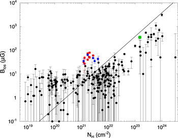
Figure 8. Line-of-sight magnetic fields Blos from Zeeman effect measurements plotted against H column densities N(H) = N(H0) + 2N(H2). Original plot taken from Crutcher (2012), who lists references. Red dots indicate Blos in H i component A, blue dots indicate Blos in H i component B, and the green dot indicates Blos in the OH-absorbing molecular gas of the northeast Dark Lane.
Download figure:
Standard image High-resolution imageThe Zeeman effect data of Figure 8 and of Tables 5 and 6 illustrate several key points. First, we exclude from consideration the colored points for the Veil. Then, magnetic field strengths (black circles) remain remarkably constant with increasing N(H) up to N(H) ≈ (1–2) × 1022 cm−2. For higher N(H), field strengths increase. Otherwise stated, λ increases systematically with increasing N(H), remaining subcritical at lower values of N(H) in the diffuse H0 gas. Above N(H) ≈ (1–2) × 1022 cm−2, λ in the molecular gas becomes nearly constant and slightly supercritical. The constancy of field strengths at lower N(H) has been noted in the past (e.g., Crutcher 2012). Lazarian et al. (2012) suggest that it is the result of the reconnection diffusion process that maintains approximately constant field strength in a gathering cloud until the free-fall timescale becomes shorter than the reconnection diffusion timescale. Once this threshold is reached, the gas contracts gravitationally, drawing in and strengthening the field in the process. We comment further on this process in Section 4.3.2.
Now considering the colored points in Figure 8 for the Veil, the green circle representing molecular gas in the northeast Dark Lane is quite consistent with other data points for molecular gas of comparable N(H). Very likely, this region of the Veil has been largely undisturbed by the star formation process, so it is typical of dense molecular gas associated with massive star formation elsewhere. However, the red and blue circles representing H i components A and B, respectively, lie a factor of 3–4 above the black circles for magnetic fields in other regions of the ISM with comparable N(H). Otherwise stated, these Veil H0 regions are more magnetically subcritical (i.e., λ smaller) than other regions of comparable N(H). See Section 4.3 for further comments about the low values of λ (i.e., high ratios B/N(H)) in these components.
4.3. The Natures of H i Velocity Components A and B
The Orion Veil offers an unusual opportunity to explore PDR physics, as noted in the Introduction. The high field strengths in the Veil compared to those in the CNM, as well as a wealth of other observational evidence (e.g., vdWGO13), clearly establish that the Veil is closely associated with the Orion star-forming region, not unrelated diffuse gas along the line of sight. Also, the Veil has apparent plane-parallel geometry perpendicular to the line of sight, and it is located nearby, so it is susceptible to high spatial resolution studies. Abel et al. (2016) constructed detailed PDR models of the Veil (see also Abel et al. 2004, 2006). From these models, they estimate n(H) ≈ 102.5 and 103.4 cm−3 and TK ≈ 50 and 60 K for components A and B, respectively. Strictly speaking, these parameters apply only to the line of sight toward the Trapezium. However, we assume that they apply to other Veil lines of sight where N(H) is comparable.
The magnetic field images in Figures 5 and 6 offer important additional perspectives on the natures of H i components A and B. These images reveal that Blos in the two H i components have very similar values and morphologies (Section 4.1). These magnetic similarities, together with the similarities in morphology of N(H0)/Tex and in velocity gradients between the two components (see vdWG89), establish that components A and B are very closely associated. However, two questions must be addressed before a comprehensive understanding of the Veil is possible. One question is the distances of components A and B from the principal source of radiation, the Trapezium stars. The second question is the origin of the relatively high magnetic field strengths in components A and B. We consider these questions in the following two subsections.
4.3.1. Locations and Natures of H i Components A and B
Several authors have concluded that H i component B lies closer to the Trapezium stars than component A. For example, vdWG89 argued that component B consists of gas heated and photodissociated by non-H-ionizing stellar photons escaping from the H+ region. In this picture, H i component A is gas that has not yet been kinematically affected by the H+ region and makes up an envelope of H0 surrounding the molecular gas. These authors also noted that the blueshift of component B relative to A (≈4 km s−1; see Section 3.2) can result from thermal expansion of the former owing to radiative heating. Recently, Abel et al. (2016) obtained high spectral resolution HST (STIS) spectra in the 1133–1335 nm wavelength range toward Theta 1B Ori. These spectra resolve H i components A and B. Abel et al. detected Veil absorption lines of CI, CI*, CI**, and rotationally/vibrationally excited H2. Based on these data, they constructed a PDR model for the Veil that yields estimates of the distances of components A and B from the Trapezium, as well as the temperatures, volume densities, and thicknesses of the two components. The model establishes that component B is, indeed, closer to the Trapezium, about 2 pc distant, as compared to 2.4 pc for component A.7 This relative placement is consistent with the facts that component B is warmer, thinner, denser, and more turbulent than component A. All of these properties point to more interactions of component B with the Trapezium environment than component A. At the same time, kinematic and magnetic similarities suggest a very close physical association between components A and B, as argued above.
One possible close physical association between the two components is that they lie on opposite sides of the shock preceding a weak-D ionization front. That is, component B is shocked gas, and component A is pre-shock gas. For this scenario to apply, we assume that the magnetic field lies nearly perpendicular to the plane of the shock (i.e., along the line of sight). Then, neglecting possible field tangling induced by motions within the shock layer itself, the shocked gas would slide along the field lines, increasing its density with no increase in magnetic field strength in component B, as observed. In such a case, standard, nonmagnetic jump conditions apply for the shock since the magnetic pressure is not relevant to motions along the field direction. We apply the equations for nonmagnetic shocks in Shu (1992), using values for n(H) and TK in components A and B derived by Abel et al. (2016; see Section 4.3 above). We estimate a shock velocity of 2 km s−1. The shock results in a blueshift of component B relative to component A of 1.7 km s−1, to be compared with the observed value of 4 km s−1. That is, the shock model underpredicts the velocity difference between the two components by a factor of about two. The predicted velocity difference is approximately proportional to [TB × n(H)B/n(H)A]½, where TB is the kinetic temperature of component B. Therefore, a two times higher predicted velocity difference would require, for example, a two times higher temperature and two times higher density ratio. Abel et al. (2016) do not provide error estimates for their photoionization model-derived values of TB, n(H)B, and n(H)A. As a result, we cannot estimate the likelihood of higher temperatures and density ratios. Also, the velocity difference between components A and B varies as a function of position across the Veil, with values closer to 3 km s−1 in some positions. In short, the shock model is attractive because it accounts for kinematic and magnetic similarities between the components, and the shock passage may account for the higher turbulence in component B than in A. However, the shock model offers an uncertain quantitative fit to photoionization model densities and temperatures of Abel et al. (2016).
We illustrate the natures and locations of Veil components A and B with the cartoon of Figure 9. In this figure, the Earth is to the left, and north is up. Neutral gas is shown in blue, ionized gas, in red. The cartoon places component B closer to the Trapezium, and the cartoon shows the thicknesses of components A and B as derived from the Abel et al. (2016) Veil model, 1.6 and 0.40 pc, respectively. According to this same model, n(H) ≈ 102.5 and 103.4 cm−3 for components A and B, respectively. The higher density of component B is suggested in Figure 9 by darker shading. Three H+ regions are shown in the figure. One is the main Orion H+ region (Orion Nebula) with a scale height of 0.05 pc (O'Dell 2001), located 0.25 pc behind the Trapezium stars (Abel et al. 2006). The vertical extent of the Orion Nebula in the cartoon represents the size of the bright Huygens region, about 0.8 pc. (The vertical extent of the Veil is arbitrary.) The second H+ region in Figure 9 is labeled "Blue-shifted H+" ("blue component" in Abel et al. 2016; also described by Abel et al. 2006). This matter-bounded, ionized layer is shifted about −25 km s−1 relative to OMC-1, and it is observed in optical emission lines and uv absorption lines. Abel et al. (2006) note that the blueshift can be ascribed to stellar radiative acceleration over a period of order 105 yr. The third H+ region, labeled "Veil H+ region," is presumed to exist on the front face of the neutral Veil. However, optical and uv tracers of this layer would lie at velocities similar to those of the Orion Nebula; hence, they are unobservable. Immediately behind the Orion Nebula lies the OMC-1 filamentary cloud and the Orion-KL core. Also shown is the Orion-S molecular core embedded within OMC-1. However, this Orion-S location is only one possibility discussed in Section 4.4 below.
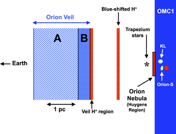
Figure 9. Cartoon of the Orion Nebula environment seen sideways (i.e., edge-on) with the Earth at left and north up. Blue regions are neutral gas, with the darkest blue representing molecular gas of OMC-1. Red regions are H+. Included in the diagram are the filamentary molecular cloud OMC-1 with the Orion-KL core and the Orion-S core within, the Orion Nebula H+ region (bright inner Huygens region), the Trapezium stars, and the Orion Veil. The Veil is shown with its two principal H0 velocity components A and B, and the presumed Veil H+ region facing the Trapezium stars. Horizontal dimensions are to approximate scale (except the width of the Veil H+ region, for which no width estimate exists). Width estimates for components A and B are from Abel et al. (2016). The vertical dimension of the Orion Nebula Huygens region is to scale; the OMC-1 cloud is a filament extending north and south of the diagram. The vertical extent of the Veil is arbitrary, although it must extend at least 1 pc above the Trapezium to cover M43. The possible location of the Orion-S core within OMC-1, hence behind the Orion Nebula, is discussed in Section 4.4. An H+ region (filled red circle) behind Orion-S is also discussed in Section 4.4. See O'Dell et al. (2009, Figure 5) for an alternate model of the location of Orion-S.
Download figure:
Standard image High-resolution imageFinally, we comment on the 21 cm H i excitation temperatures Tex in components A and B in comparison with their kinetic temperatures. Under typical conditions in the galactic ISM, it is commonly expected that Tex ≈ TK. However, under conditions of low density and/or high stellar uv flux, resonant scattering of Lyα photons can pump the H i levels, increasing Tex above TK (Field 1959). Veil components A and B offer an unusual opportunity to study this effect since both Tex and TK are independently known along the line of sight to the Trapezium. In particular, Tex ≈ 90 and 135 K for components A and B, respectively (Abel et al. 2006), while TK ≈ 50 and 60 K for components A and B, respectively (Abel et al. 2016; see above). Therefore, the H i levels have been pumped in both components, and more so in component B, as one would expect if this component is closer to the Trapezium and subject to a higher stellar uv flux. However, it is not possible to be more quantitative about the pumping effect. The magnitude of the effect depends on the unknown strengths of the Lyman lines in the stellar spectral energy distribution (SED; Abel et al. 2016).
4.3.2. Magnetic Fields in the H i Components—Precursors and/or Products of Star Formation
Magnetic field strengths in Veil H i components A and B are anomalous compared to those measured elsewhere in the ISM in three ways: (1) The ratio B/N(H) is 3–4 times higher in these components than it is in other regions in the ISM of comparable N(H), as indicated in Section 4.2 and Figure 8. Equivalently stated, λ ∝ N(H)/B is 3–4 times lower; hence, the gas is subcritical. (2) Component A is uniquely sub-Alfvénic, that is, turbulent energy is much weaker than magnetic energy, also described in Section 4.2. (3) The ratio B/n(H) in component A is about a factor of 5 higher than it is in other regions of the ISM with comparable n(H). This third anomaly is based on a statistical analysis of Zeeman effect data done by Crutcher et al. (2010). The analysis suggests that Btot in the ISM ranges from near zero to a maximum value  , where
  is a function of n(H). For n(H) < n0(H) ≈ 300 cm−3,
  ≈ 10 μG. For n(H) > n0(H),
  ≈ 10 × [n(H)/n0(H)]0.65 μG. This exponent (2/3, more specifically) is expected for isotropic collapse of a flux-frozen cloud (Mestel 1966). Observed values of log Blos as a function of log n(H) are plotted in Figure 1 of Crutcher et al. (2010). The solid line in this figure (horizontal and diagonal) represents the best fit to the Zeeman effect data for
  . Given the model-derived density for H i component A (n(H) ≈ 102.5 cm−3; Section 4.3), the best-fit line predicts
  ≈ 10 μG, one-fifth the measured Blos ≈ 50 μG. The challenge presented by these three magnetic anomalies is to explain them in terms of the history of the Veil H i gas. This history begins with gravitational contraction of OMC-1 prior to star formation. The history continues with the effects of a strong stellar radiation field after star formation. Magnetic fields in the Veil today may be precursors and/or products of star formation in OMC-1. We explore these two possibilities below.
We first consider Veil H i magnetic fields as precursors to star formation. We focus on H i component A since it is less likely to have been affected by the Trapezium stellar environment (Section 4.3.1). The higher ratio B/n(H) in component A (anomaly c above) could be an effect of reconnection diffusion, assuming that the Veil precursor gas existed in a low-turbulence environment. Reconnection diffusion is proposed as a way to remove magnetic flux from turbulent clouds. This process may explain the insensitivity of B to n(H) for n(H) < 102–103 cm−3 (Lazarian et al. 2012). In this scenario, field strengths remain roughly constant as cloud material gathers into a giant molecular cloud since reconnection diffusion removes magnetic flux. As n(H) increases, field strengths eventually begin to rise once n(H) reaches a critical value no(H). The rise in field strength begins once the free-fall timescale (∝1/n(H)½) becomes shorter than the reconnection diffusion timescale (∝1/ΔVturb, where ΔVturb is the turbulent velocity dispersion). Therefore, no(H) is proportional to  . If ΔVturb was comparatively low in the OMC-1 precursor gas, then the magnetic field began rising at a comparatively low value of no(H), leading eventually to a higher ratio B/n(H), as observed in Veil component A. Since the ratio B/n(H) is higher in component A by a factor of ≈5, we estimate that no(H) for the precursor gas is ≈30 cm−3. That is, reconnection diffusion ceased to remove magnetic flux in the Veil precursor cloud once n(H) reached 30 cm−3, and then, presumably, B increased as n(H)0.65. This behavior can be visualized by a modification to Figure 1 of Crutcher et al. (2010). In this plot of log Blos versus log n(H), we place a horizontal line at 10 μG for n(H) < 30 cm−3. For n(H) > 30 cm−3, we place a diagonal line representing B ∝ n(H)0.65, the same slope actually shown in the figure for n(H) > 300 cm−3. With this modification, the figure now predicts
  ≈ 50 μG for the estimated n(H) of H i component A. This field strength is (by design) the same as the Zeeman effect measurement for Blos. Since n0(H) in the Veil precursor gas was about 1/10 the usual value for the ISM (i.e., 30 versus 300 cm−3), the turbulent velocity in the Veil precursor gas was about one-third the usual value, given that n0(H) ∝
  , as noted above. The same reconnection diffusion process can also account for the higher ratio B/N(H) in the Veil (anomaly a above). For the ensemble of non-Veil Zeeman effect data,
  ∝ N(H) once N(H) > N0(H) ≈ 1022 cm−2 (Figure 8). Since the ratio B/N(H) is higher for Veil component A by a factor of ≈4, we estimate that N0(H) for the gas that eventually became part of this component is ≈2.5 × 1021 cm−2.
We conclude that reconnection diffusion in a low-turbulence environment can explain the higher ratios B/n(H) and B/N(H) observed in the Veil H i component A compared to these ratios in the ensemble of non-Veil Zeeman data. In such a low-turbulence environment, field strengths in OMC-1 begin rising at lower values of n(H) and N(H) than they do in more typical interstellar environments. The low-turbulence hypothesis is consistent with the finding that the Alfvénic Mach number is ≪1 in component A, a unique property among regions probed by the Zeeman effect to date (Section 4.2). The origin of low turbulence in OMC-1 could be related to the distance of the cloud above the galactic plane (150 pc). Molecular gas so high above the plane may be less subject to the input of mechanical energy from adjacent star formation and supernovae than molecular gas closer to the plane.
Now we consider Veil H i magnetic fields as products of star formation, that is, the effects of nearby early-type stars on the Veil magnetic fields. Pellegrini et al. (2007) describe a model in which magnetic pressure in PDRs resists the momentum of absorbed starlight (far-UV and EUV) and the pressure of adjacent hot (106 K), X-ray-emitting gas from shocked stellar winds (see also Ferland 2009). In this model, the PDR is compressed by starlight momentum and hot gas pressure. As a result, the magnetic field is also compressed, raising the field strength and magnetic pressure. Since magnetic pressure is proportional to B2, the magnetic pressure increases faster than the gas pressure for most geometries. Eventually, the magnetic pressure dominates the total pressure in the PDR and establishes an approximate magnetostatic equilibrium. Note that this process requires some component of B to lie in the plane of the Veil PDR (i.e., perpendicular to the line of sight) since it is this field component that can be amplified by compression of the PDR. The Pellegrini et al. model also results in an increase in B/N(H), as observed in Veil components A and B, since compression of the PDR increases B but not N(H). Pellegrini et al. used the spectral synthesis code Cloudy (Ferland et al. 1998, 2013) to model the M17 PDR along the lines described above. They successfully reproduced magnetic field strengths previously observed with the VLA via the H i Zeeman effect.
To apply the Pellegrini et al. concepts to the Veil, we use an approximate technique (as opposed to a full Cloudy model) to estimate field strengths in the Veil H i regions. We estimate field strengths by equating magnetic pressure (B2/8π) to radiation pressure plus the pressure of X-ray-emitting gas. Radiation pressure is given by F/c, where F is the flux (erg cm−2 s−1) integrated over a specified wavelength band and incident on the PDR. We distinguish between FEUV (flux of H-ionizing radiation) and FFUV (uv flux of non-H-ionizing radiation). Also, the pressure of the hot gas Px = nkTx, where Tx is the kinetic temperature. Equating magnetic pressure to radiation pressure plus hot gas pressure, we arrive at the predicted PDR field strength BPDR = (8π)½ (FEUV/c + FFUV/c + Px)½, all in cgs units. This relation is equivalent to Equation (7) of Pellegrini et al., except we also include the effects of the non-ionizing radiation FFUV. To estimate FEUV and FFUV for the Orion Veil, we use the Trapezium SED derived by Abel et al. (2016) and assume that the Veil is 2 pc from the Trapezium (Section 4.3.1). Thus, we find FEUV ≈ 0.54 erg cm−2 s−1 and FFUV ≈ 1.5 erg cm−2 s−1. We take Px/k = 106 K cm−3, based on the Orion X-ray observations of Güdel et al. (2008). This estimate for Px is rather uncertain because the properties of the hot gas immediately adjacent to the Veil are not well constrained by the X-ray observations. With these parameters, we predict BPDR ≈ 70 μG, including radiation and hot gas pressure, and BPDR ≈ 40 μG if only radiation pressure is included. These magnetic field strengths are comparable to those measured in H i components A and B. We conclude that a model in which the Veil PDR is magnetically supported against stellar radiation and hot gas pressures is consistent with the H i Zeeman effect observations. Mayo & Troland (2012) applied this same concept to the PDR associated with H+ region DR22.
The implications of such a magnetically supported PDR model, along the lines described by Pellegrini et al. (2007), are twofold. First, the model suggests that the currently observed magnetic fields in the H i Veil may have been increased by the presence of nearby early-type stars. If the initial field strengths in the Veil PDR were insufficient to support it against radiation pressure and X-ray-emitting gas from the Trapezium, then the PDR would have been compressed, raising the field strength until equilibrium was achieved. This process would increase the ratio B/N(H), as observed; however, it would not increase the ratio B/n(H). Of course, OMC-1 cloud evolution may have led to equilibrium level field strengths prior to star formation as described above. In such a case, no further compression of the PDR and enhancement of B would have been necessary. The other, more general implication of the magnetically supported PDR model is that magnetic fields can play an important role in establishing physical conditions within these regions. Since magnetic pressure is dominant in such a PDR model, gas pressure, and hence gas density, is lower than it would be in a nonmagnetic environment. As a result, the magnetized H0 (for a given N(H)) extends more deeply into the PDR. That is, the dominance of magnetic pressure in the H0 gas significantly affects physical conditions there, creating a deeper, lower-density atomic layer than expected in the nonmagnetic case. If so, then PDR models that do not account for magnetic pressure may significantly underestimate the depths and overestimate the gas densities in the H0 regions.
4.4. The Location of Orion-S
Orion-S is one of two high-mass molecular cores in OMC-1; Orion-KL is the other. Orion-S is 90'' south of Orion-KL and about 60'' southwest of the Trapezium cluster (see Section 3.3 and Figure 2). Like Orion-KL, Orion-S is clearly visible in images of submillimeter dust emission (Lis et al. 1998; Johnstone & Bally 1999) and in molecular emission line images (e.g., Peng et al. 2012). The 850 μm dust emission image of Johnstone & Bally (see contour image in Peng et al. 2012) reveals an Orion-S core approximately 40'' (0.09 pc) in diameter, with N(H) ≈ (2–4) × 1024 cm−2 (Av ≈ 800–1600 mag). The factor of two uncertainty reflects uncertainties in theoretically calculated values of the dust opacity κν. Other uncertainties exist in this N(H) estimate, for example, in Tdust, which we have taken as 40 K (O'Dell et al. 2009). The implied total mass for Orion-S is 130–260 solar masses; the average density, assuming spherical symmetry, is (1–2) × 107 cm−3. The virial mass of Orion-S, for an observed ΔV ≈ 5 km s−1 and radius of 0.05 pc, is about 150 solar masses, suggesting that the core is close to virial stability.
It is logical to imagine that Orion-S lies behind the main Orion H+ region, just like the Orion-KL core. For example, there is no obvious optical extinction feature associated with this optically opaque core, just as there is none for Orion-KL. However, the situation for Orion-S is more complicated owing to several discoveries reported in the previous literature. Johnston et al. (1983) and Mangum et al. (1993) found 6 cm (4.8 GHz) H2CO absorption toward Orion-S. The present OH data also reveal absorption (Section 3.3). The present data also show H i absorption toward Orion-S, and the data of vdWGO13 show this same absorption at higher spatial resolution (identified by these authors as H i component H). We illustrate the clear kinematical association between OH and H i absorption and Orion-S molecular emission in Figure 10. This figure presents H i and OH optical depth profiles from the present work and a CS (2-1) emission profile from Tatematsu et al. (1998). See the figure caption for beamwidths and channel separations. All three profiles are toward the center position of Orion-S. The OH and CS profiles have nearly identical center velocities (7 km s−1) and velocity widths. The H i profile has a weak component on the high-velocity side of the main velocity component that appears to match the OH and CS features. (The low-velocity side of this weak H i component, at velocities 3–7 km s−1, is presumably obscured by the main H i velocity component.) Evidently, a source of radio continuum emission lies behind all or part of Orion-S in order to account for the H i, OH, and H2CO absorption. Most likely, this radio continuum emission comes from an H+ region. Another indication of the complexity of the Orion-S core comes from anomalies in the optical extinction reported by O'Dell et al. (2009). These anomalies suggest that part of the radio continuum observed toward Orion-S comes from an ionized layer from which we receive no Hα light. Presumably, this H+ layer lies behind an optically opaque layer associated with Orion-S. In short, previous and present observations point to the presence of two distinct layers of H+ along the line of sight to Orion-S. These layers are separated by an optically opaque region that consists of all or part of Orion-S.
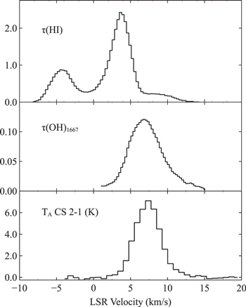
Figure 10. Profiles toward center of Orion-S for H i optical depth (top), 1667 MHz OH optical depth (middle), and CS (2-1) emission (bottom). H i and OH profiles come from the present work. See Tables 1 and 2 for beamwidths and channel separations. CS profile is from Tatematsu et al. (1998); beamwidth is 50'', and channel separation is 0.75 km s−1.
Download figure:
Standard image High-resolution imageApart from kinematics (Figure 10), there is an intriguing spatial correspondence between the H i absorption and the Orion-S core defined by dust emission. The vdWGO13 data offer a high spatial resolution image of this absorption. In Figure 11 we overlay contours of the 850 μm dust emission (dashed contours; Johnstone & Bally 1999) on an image of H i optical depth from the data of vdWGO13 (colors and light contours). The H i optical depth image has been integrated over the velocity range 8.4–9.7 km s−1, a range over which optical depth associated with Orion-S is uncontaminated by unrelated velocity features (see Figure 10, top panel). The H i image has a synthesized beamwidth of 6 4. Figure 11 shows that the H i absorption arises from a partial shell just to the west of the peak in 850 μm dust emission associated with Orion-S. Although the morphologies of 850 μm dust emission and H i optical depth are far from identical, the general correspondence between the two provides strong evidence, along with the kinematical evidence (Figure 10), that the H i absorption is closely associated with Orion-S. The same conclusion holds for the H2CO and OH absorption.

Figure 11. H i optical depth averaged over the velocity range 8.4–9.7 km s−1, taken from data of vdWGO13 (colors and light contours). Synthesized beamwidth is 64. Optical depth contours are for 0.1, 0.2, 0.3, and 0.4 napiers. Pixels with indeterminate optical depth have been set to zero. Overlaid are contours for 850 μm JCMT/SCUBA dust continuum emission from data of Johnstone & Bally (1999), as plotted by Peng et al. (2012). Dust emission contours (heavy, dashed lines) are for 7%, 20%, 40%, and 80% of the peak flux of 87 Jy beam−1, where the beamwidth is 14''. Locations of Orion-KL and Orion-S in the 850 μm image are indicated.
Download figure:
Standard image High-resolution image
O'Dell et al. (2009) propose that Orion-S is an isolated molecular core lying in front of the main ionization front (MIF) of the Orion Nebula (see their Figure 5). Therefore, the main H+ region provides radio continuum absorbed by H2CO, OH, and H i. In this model, light from the Trapezium cluster ionizes the front face of Orion-S. As seen from the Earth, light from this ionized Orion-S layer fills in light from the main H+ region that is blocked by Orion-S. Therefore, Orion-S does not create an obvious optical extinction feature even though it lies in front of the MIF. O'Dell et al. also provide a detailed spectral synthesis calculation of Orion-S, predicting the run of density, dust and gas temperatures, and chemical composition into the core. This model establishes, for example, that Tdust in the core remains above the 30 K needed to keep H2CO from freezing out onto grains.
Several objections can be raised to the O'Dell et al. (2009) model, none of which exclude it. These objections are related to the need for ionized gas behind Orion-S to account for the atomic and molecular absorption. In the O'Dell et al. (2009) model, the position of Orion-S must be carefully chosen so that it does not shadow the main Orion H+ region behind it. If Orion-S were to shadow this layer, then the layer would not be ionized, so it could not emit the radio continuum. Also, such a shadow would likely be visible in optical images of the Orion Nebula to the southwest of Orion-S (i.e., opposite to the direction toward the Trapezium). No such shadow is apparent (Figure 1(a), southwest of position OH4 that is coincident with Orion-S). Indeed, the existence of an isolated molecular core in Orion, surrounded by H+, seems unlikely. Most of the ionizing radiation in Orion comes from a single star, Theta 1C Ori. Therefore, Orion-S must cast a shadow, creating an elephant trunk of neutral gas similar to those observed in M16 (Hester et al. 1996). The postulated Orion-S elephant trunk would be seen from a different angle than those of M16. The Orion-S structure would point more nearly toward the observer in Orion and be seen against the bright background of the main H+ region. This geometry would be quite unlike that of the M16 elephant trunks that lie approximately in the plane of the sky and are viewed against a darker background. As a result, the Orion-S elephant trunk might be much less visible in optical images than those of M16. Nonetheless, an Orion-S elephant trunk would have to be carefully positioned to account for H+ behind the Orion-S core. With a suitable choice of geometry, this background H+ gas could be part of the main Orion H+ region, or it could lie along the skin of the elephant trunk on the side of the structure facing away from Earth. Either way, the geometry of the Orion elephant trunk would have to be rather optimally configured in order to place a significant amount of ionized gas directly behind Orion-S, while Orion-S itself lay in front of the MIF.
We now offer another explanation for the presence of H i, OH, and H2CO absorption toward Orion-S that avoids the need to carefully position the molecular core in front of the MIF. In this model, the Orion-S molecular core lies entirely behind the MIF, just like Orion-KL. On the back side of Orion-S (i.e., facing away from Earth), an early-type star has created a small H+ region whose radio continuum emission is responsible for the observed atomic and molecular absorption. The small H+ region could be a blister-type region, similar to but smaller than the Orion Nebula, or it could be embedded within Orion-S. We have made a simple estimate of the type of star that could form such a small H+ region. We use the formalism described by Jackson & Kraemer (1999) and references therein. Consider an H+ region as large as Orion-S (0.1 pc) in the plane of the sky. Suppose that this H+ region has half the radio continuum brightness (in Jy beam−1) as the main Orion H+ region. (Were the small H+ region much brighter, it would create an obvious peak in total brightness toward Orion-S, contrary to observation.) Given the assumed brightness and size of the small H+ region, its total 21 cm flux density is about 4 Jy. Assuming an electron temperature Te ≈ 8000 K, the small H+ region could be created by a B0 zero-age main-sequence star, a star far less luminous than Theta 1C Ori. Such a star, on the back side of Orion-S or embedded within it, would be invisible behind Av ≈ 1000 from Orion-S. The postulated Orion-S H+ region is shown in Figure 9 as a red circle immediately behind Orion-S.
This second Orion-S model is ad hoc but plausible on several grounds. For one, Orion-S is well established as a star-forming region (e.g., Henney et al. 2007). Therefore, the presence of a B0 star in its vicinity would be no surprise. Also, the roughly circular region of enhanced optical extinction in the image of O'Dell & Yusef-Zadeh (2000) is easily explained as an artifact arising from background radio continuum emission of a small Orion-S H+ region from which no Hα emission is observed owing to the large optical extinction of Orion-S in front. (This is the anomalous extinction phenomenon cited above and described by O'Dell et al. 2009.) Finally, the partial shell of H i optical depth adjacent to Orion-S (see above) can be naturally explained as arising in a partial shell of H0 gas lying just outside the small Orion-S H+ region. In this simple model, the Orion-S core is just like the Orion-KL core, behind the main Orion H+ region. If this model is correct, then the Orion-S core may lie just barely behind the main Orion H+ region. Orion-S coincides spatially with a local maximum or bump in the H+ region surface that points toward Earth. This bump appears in the 3D map of Wen & O'Dell (1995). These authors note that the bump could be caused by dense gas behind the H+ region that retards the advance of the ionization front. This dense gas, of course, would be the Orion-S molecular core.
In short, two different models of Orion-S can account for existing observations, especially the presence of atomic and molecular absorption associated with the core. One model (O'Dell et al. 2009) places Orion-S in front of the MIF, as an isolated neutral region immersed in H+ gas. It is only a slight modification of this model (described above) to replace the isolated core with an elephant trunk having the core at its tip. The other model (present work) places Orion-S behind the MIF (like Orion-KL) with yet another, smaller H+ region behind Orion-S. Both models require ad hoc assumptions. However, we favor the placement of Orion-S behind the MIF since this placement avoids the necessity of rather specific geometry of an isolated molecular region or elephant trunk. Future high spatial resolution images of the atomic and molecular absorption regions associated with Orion-S might assist in distinguishing between these two models. For example, if the morphologies of H i and molecular absorption are found to trace a partial shell around the molecular core (a circumstance hinted at in Figure 11), this result would strengthen the hypothesis that a small H+ region lies behind Orion-S and a partial shell of neutral gas surrounds the ionized gas. That is, this result would strengthen the model placing Orion-S behind the MIF.
5. SUMMARY AND CONCLUSIONS
The Orion Veil is a mostly atomic PDR that lies about 2 pc in front of the Orion Trapezium stars (as viewed from Earth) and nearly perpendicular to the line of sight. The Veil covers all of the Orion Nebula and extends at least as far northeast as the smaller H+ region M43. Radio, optical, and UV absorption lines from the Veil provide an unusual opportunity to study PDR physical conditions. These lines reveal two principle H i velocity components, labeled A and B. We report aperture synthesis observations of the Zeeman effect in 21 cm H i absorption lines and in 18 cm (1665 and 1667 MHz) OH absorption lines across the Veil. The H i data yield independent images of the line-of-sight magnetic field strength Blos in components A and B with a synthesized beamwidth of 25''. The OH data provide a measurement of Blos in an optically obscured molecular region of the Veil along the northeast edge of the Orion Nebula. The synthesized beamwidth of the OH observations is 40''.
From the H i Zeeman data, we find Blos ≈ −50 to −75 μG across much of the Veil, rising to about −300 μG toward the northeast Dark Lane, a region of high optical obscuration along the northeast edge of the Orion Nebula (Section 3.4). Images of Blos for H i velocity components A and B (Figures 5 and 6) are very similar. This similarity suggests a close association between the atomic layers responsible for the two components. From the OH Zeeman data, we find Blos = −350 ± 47 μG in molecular gas of the northeast Dark Lane (Section 3.5) at a position where Blos,H i is −183 ± 32 μG in H i component A.
We assess the importance of thermal, turbulent, magnetic, and gravitational energies in the Veil and compare these energies with energies in other locales of the ISM (Section 4.2, Tables 5 and 6). H i components A and B have mild supersonic turbulence (Mturb ≈ 3), similar to the CNM. However, molecular gas in the Veil has much stronger supersonic turbulence (Mturb ≈ 4–6), similar to molecular gas in other regions of high-mass star formation. Thermal energy is insignificant in H i components A and B compared to magnetic energy (βtherm ≪ 1), as it is in most of the ISM. An approximate balance exists between turbulent and magnetic energies in much of the atomic and molecular gas of the Veil, just as it does in other regions the ISM probed with the Zeeman effect (trans-Alfvénic turbulence, βturb ≈ 1, MA ≈ 1). However, H i component A is uniquely sub-Alfvénic (βturb ≈ 0.02, MA ≈ 0.1); magnetic energy strongly dominates turbulent energy. We estimate the mass-to-flux ratio (ratio of gravitational to magnetic energies) of gas in the Veil. Veil H i components A and B are magnetically subcritical (λ < 1, magnetically dominated), similar to the CNM, where n(H) is about 1 dex lower. The molecular gas of the Veil, where sampled by the Zeeman effect, appears magnetically critical to supercritical (λ ≥ 1, gravitational energy comparable to or greater than magnetic energy), like molecular gas in other regions of high- and low-mass star formation.
We consider the physical nature of H i components A and B (Section 4.3). Like previous authors, we argue that component B is closer to the Trapezium stars than component A (see Figure 9). This placement explains why component B is warmer, denser, and more turbulent than component A. Component B may consist of post-shock gas associated with a weak-D ionization front, its blueshift relative to component A arising from the passing shock that precedes the ionization front. This model requires the magnetic field in both components to lie nearly along the line of sight (i.e., perpendicular to the shock front).
Magnetic fields in H i components A and B are anomalous in the sense that they are 3–5 times stronger than fields in other regions of the ISM with comparable N(H) and n(H). See Section 4.3.2 and Figure 8. One explanation for these anomalies lies in the history of OMC-1 before star formation. If OMC-1 was formed in an unusually low turbulence environment (perhaps because of its position 150 pc above the galactic plane), then the process of reconnection diffusion was less efficient at removing magnetic flux from the developing cloud. As a result, gravitational contraction began at lower values of n(H) and N(H), leading to higher ratios B/N(H) and B/n(H) today. This hypothesis is consistent with the low Alfvénic Mach number in H i component A (i.e., low turbulent energy) since this gas likely samples material in OMC-1 that has yet to be disturbed by the Trapezium stars. Another explanation for the magnetic anomalies of H i components A and B lies in events that occurred after star formation. Pressure from starlight and from adjacent hot (106 K) gas can compress the PDR, raising field strengths within it until a magnetostatic equilibrium is achieved. We find that field strengths in components A and B are consistent with such an equilibrium.
Finally, we consider the location of the Orion-S molecular core (Section 4.4). This massive core (M ≈ 200 MSun, N(H) ≈ 3 × 1024 cm−2) is similar in nature to Orion-KL. However, the Orion-S location is unclear. The existence of H i and molecular absorption lines spatially and kinematically associated with Orion-S (Figures 10, 11) establishes that a source of radio continuum lies behind the core. O'Dell et al. (2009) propose that Orion-S is an isolated core lying in front of the MIF of the H+ region. We note several possible objections to this idea, none of which rule it out. We prefer another location for Orion-S, placing the core behind the MIF, with another, smaller H+ region behind or embedded within Orion-S. Future high spatial resolution observations of the atomic and molecular absorption lines may help distinguish between these two models.
We gratefully acknowledge the careful reading of an early version of this manuscript by CR O'Dell, as well as his numerous comments and suggestions. This work has been supported in part by NSF grant AST 0908841 to T.H.T. We also acknowledge the referee's thorough reading of the manuscript and his or her constructive suggestions.
Footnotes
- 6
The National Radio Astronomy Observatory is a facility of the National Science Foundation operated under cooperative agreement by Associated Universities, Inc.
- 7