


ABSTRACT
We study the relationship between stellar mass, star formation rate (SFR), ionization state, and gas-phase metallicity for a sample of 41 normal star-forming galaxies at 3 ≲ z ≲ 3.7. The gas-phase oxygen abundance, ionization parameter, and electron density of ionized gas are derived from rest-frame optical strong emission lines measured on near-infrared spectra obtained with Keck/Multi-Object Spectrograph for Infra-Red Exploration. We remove the effect of these strong emission lines in the broadband fluxes to compute stellar masses via spectral energy distribution fitting, while the SFR is derived from the dust-corrected ultraviolet luminosity. The ionization parameter is weakly correlated with the specific SFR, but otherwise the ionization parameter and electron density do not correlate with other global galaxy properties such as stellar mass, SFR, and metallicity. The mass–metallicity relation (MZR) at z ≃ 3.3 shows lower metallicity by ≃0.7 dex than that at z = 0 at the same stellar mass. Our sample shows an offset by ≃0.3 dex from the locally defined mass–metallicity–SFR relation, indicating that simply extrapolating such a relation to higher redshift may predict an incorrect evolution of MZR. Furthermore, within the uncertainties we find no SFR–metallicity correlation, suggesting a less important role of SFR in controlling the metallicity at high redshift. We finally investigate the redshift evolution of the MZR by using the model by Lilly et al., finding that the observed evolution from z = 0 to z ≃ 3.3 can be accounted for by the model assuming a weak redshift evolution of the star formation efficiency.
Export citation and abstract BibTeX RIS
1. INTRODUCTION
It is well established that, up to redshift z ≃ 6, the star formation rate (SFR) of star-forming galaxies (SFGs) tightly correlates with their stellar mass (M⋆), producing a so-called star-forming main sequence (MS) where the specific SFR (sSFR ≡ SFR/M⋆) depends only weakly on stellar mass (e.g., Brinchmann et al. 2004; Daddi et al. 2007; Elbaz et al. 2007; Noeske et al. 2007; Pannella et al. 2009, 2015; Magdis et al. 2010; Peng et al. 2010; Karim et al. 2011; Rodighiero et al. 2011, 2014; Whitaker et al. 2012, 2014; Kashino et al. 2013; González et al. 2014; Speagle et al. 2014; Steinhardt et al. 2014; Renzini & Peng 2015). While the normalization of the MS increases by a factor of ≳20 from z = 0 to z = 2, the scatter (≃0.3 dex) and slope of the MS are almost independent of redshift over the entire 0 ≲ z ≲ 4 period (e.g., Salmi et al. 2012; Speagle et al. 2014; Schreiber et al. 2015). At z ≃ 2, the fraction of starbursts defined as SFGs with more than 4 times higher SFR than that of the MS is observationally constrained to be ∼2% of the total star-forming population, and they account for ∼10% of the cosmic SFR density (Rodighiero et al. 2011), and these fractions appear to be constant up to z ≃ 4 (Schreiber et al. 2015). This indicates that galaxies spend most of their star-forming phases on the MS owing to the interplay of gas inflow, star formation, and gas outflow (e.g., Tacchella et al. 2016a).
The evolution of galaxies on the MS can be attributed to the evolution of baryon accretion into dark matter halos (e.g., Dutton et al. 2010; Davé et al. 2012; Dekel et al. 2013; Lilly et al. 2013; Forbes et al. 2014; Sparre et al. 2015). Cosmological hydrodynamical simulations are able to reproduce the confinement of SFGs on the MS, with galaxies fluctuating within the observed SFR scatter of the MS in response to fluctuations in the accretion rate (Tacchella et al. 2016a). The simulations can also naturally reproduce the observed trend of the so-called inside-out quenching (e.g., Morishita et al. 2015; Nelson et al. 2015; Tacchella et al. 2015a, 2016b): in the early phase the stellar mass profile grows in a self-similar manner, i.e., no or little radial dependence of the sSFR. Then the sSFR in the central part starts being suppressed, once the central density of the bulge reaches a critical value of ≳1010 M⊙ kpc−2, at the expense of having consumed most of the gas, while star formation and mass growth still continue in the disk (Tacchella et al. 2015b). Eventually, the suppression of star formation takes place in the entire galaxy (Tacchella et al. 2015a; Carollo et al. 2016; S. Lilly & M. Carollo 2016, in preparation). This process appears to be rapid at early cosmic times, i.e., z ≳ 2, with a timescale of <1 Gyr for massive (M ≳ 1011 M⊙) galaxies (e.g., Onodera et al. 2010b, 2012, 2015; van de Sande et al. 2013; Belli et al. 2015; Barro et al. 2016), while the timescale becomes longer for less massive galaxies at later cosmic times, i.e., z ≲ 2 (e.g., Thomas et al. 2005, 2010; McDermid et al. 2015; Tacchella et al. 2015a). Therefore, less massive SFGs will stay on the MS longer before the cessation of star formation, increasing the quenched galaxy population at later epochs (Carollo et al. 2013).
Star formation enriches the gas metal content via supernova explosions and stellar mass loss, and a tight correlation between galaxy stellar mass and gas-phase metallicity (Z) in SFGs has been known since the 1970s (e.g., Lequeux et al. 1979). The stellar mass–gas-phase metallicity relation (MZR) is now well established for galaxies in the local universe (Tremonti et al. 2004). Studies of the MZR at high redshifts find systematically lower gas-phase metallicities than in their local counterparts at a given stellar mass, by up to ≃0.8 dex at z ≃ 3 (e.g., Carollo & Lilly 2001; Lilly et al. 2003; Kobulnicky & Kewley 2004; Savaglio et al. 2005; Erb et al. 2006a; Maiolino et al. 2008; Mannucci et al. 2009; Yoshikawa et al. 2010; Yabe et al. 2012, 2014; Henry et al. 2013; Cullen et al. 2014; Maier et al. 2014; Masters et al. 2014; Steidel et al. 2014; Troncoso et al. 2014; Wuyts et al. 2014; Zahid et al. 2014; Sanders et al. 2015; see also Hayashi et al. 2009; Onodera et al. 2010a).
The MS and the MZR are likely to be closely related to each other. There is indeed some evidence that the metallicity depends also on SFR as a second parameter in the MZR, leading to a  relation (Ellison et al. 2008; Lara-López et al. 2010; Mannucci et al. 2010). These authors found that local SFGs lie on a thin two-dimensional (2D) surface in the three-dimensional (3D) M–Z–SFR space, with a strikingly small scatter, only 0.05 dex, in metallicity. This surface, dubbed the "fundamental metallicity relation" (FMR), has been suggested to accommodate SFGs up to z ≃ 2.5 (Mannucci et al. 2010; Belli et al. 2013; but see Wuyts et al. 2014), even as the typical SFR at a given stellar mass is higher by a factor of ∼20.
The presence of SFR as a second parameter in the MZR follows quite naturally if star formation in galaxies is regulated by their gas reservoir (Bouché et al. 2010; Davé et al. 2012; Krumholz & Dekel 2012; Dayal et al. 2013; Lilly et al. 2013; Forbes et al. 2014). A redshift-independent  relation is theoretically predicted if the parameters of the regulator, i.e., the mass loading of the wind outflow and the star formation efficiency, are roughly constant in time. Such a gas-regulated model also links the decline of the sSFR in galaxies to the decline of the specific accretion rate of dark matter halos (with an offset of about a factor of two; Lilly et al. 2013). In this gas-regulation model the gas-consumption timescale, which is observationally estimated to be ≲1 Gyr for MS galaxies (e.g., Daddi et al. 2010; Genzel et al. 2010), is shorter than the mass increase timescale, i.e., sSFR−1, so that a quasi-steady state is maintained between inflow, star formation, and outflow. However, at very high redshifts, z ≳ 3, the gas regulator may break down as a number of timescales tend to converge, namely, the gas depletion timescale, the halo dynamical time, and the mass increase timescale of galaxies. An important diagnostic of this breakdown may come from changes in the
  relation.
Some indication that the fundamental  relation breaks down at z > 2.5 has indeed been reported (Mannucci et al. 2010; Troncoso et al. 2014). However, the samples studied so far at z > 2.5 do not include the most massive galaxies, i.e., M ≃ 1011 M⊙, despite the claim that the evolution of the
  relation may be more prominent at the high stellar mass regime (Troncoso et al. 2014; but see Zahid et al. 2014). Also, this depends on how the local
  relation is extrapolated into regions of (M⋆, SFR) that are poorly populated at low redshifts (i.e., high stellar mass and high SFR; Maier et al. 2014).
Therefore, firmly establishing whether, and with which functional form, the  relation extends beyond z ∼ 3 could provide an important clue on the regulation of star formation in galaxies at such earlier epochs. In order to properly assess the existence and form of a
  relation at z ≳ 3, it is essential to measure gas metallicities for a large number of galaxies spanning a broad range of stellar mass and SFR, including also a fair number of the most massive objects.
In this study, we use the Multi-Object Spectrograph for Infra-Red Exploration (MOSFIRE; McLean et al. 2010, 2012) on the Keck I telescope to obtain rest-frame optical emission lines that enable us to measure the gas-phase oxygen abundance,  , for a sample of SFGs at 3 ≲ z ≲ 3.7.
Compared to the previous study of Troncoso et al. (2014), our sample and data offer several advantages: galaxies are selected in a single field, i.e., the COSMOS field, enabling us to use homogeneous multiband photometry; our sample includes more objects with measured metallicity and extends to M⋆ ≃ 1011 M⊙; resolving the [O ii] λλ3726, 3729 doublet allows us to estimate the electron density of the ionized gas. Using the measured metallicity and wealth of a multiwavelength data set, we then study the  relation at the critical epoch to test the gas-regulator model of star formation in galaxies.
In Section 2, we introduce our data used in this study. Basic measurements of emission lines, AGN contamination, spectral energy distribution (SED) fitting, SFR, and spectral stacking procedure are presented in Section 3, and measurements of the ionized gas properties are reported in Section 4. In Section 5, we discuss the relation between the ionized gas properties and other galaxy properties such as stellar mass and SFR. We summarize our results in Section 6.
Throughout the analysis, we adopt a Λ-dominated cold dark matter (ΛCDM) cosmology with cosmological parameters of H0 = 70  Mpc−1, Ωm = 0.3, and ΩΛ = 0.7 and the AB magnitude system (Oke & Gunn 1983). Unless explicitly stated, we use the terms "metallicity" and "Z" to express "gas-phase oxygen abundance" or "
 ," and we use a base 10 for logarithm.
2. DATA
2.1. Sample Selection
Our primary goal of the project is to measure metallicity at z ≳ 3 using strong rest-frame optical emission lines such as [O ii] λλ3726, 3729,  , and [O iii] λλ4959, 5007. At 3 < z < 3.8, [O ii] λλ3726, 3729 are observed in H band and
  and [O iii] λλ4959, 5007 can be accessible in K band.
Our primary sample has been extracted from the zCOSMOS-Deep redshift catalog (Lilly et al. 2007, and in preparation).
We have first selected objects in the redshift range 3 < zspec < 3.8 that are spectroscopically classified as galaxies (i.e., neither stars nor broad-line AGNs), and the redshifts are reliable with confidence classes (CC) in the range of 2.5 ≤ CC ≤ 4.5, which includes some insecure spectroscopic redshifts but agrees well with photometric redshifts (see Table 1 in Lilly et al. 2009). Then we have given higher priority to those with the expected line positions of [O ii] λ3727,  , and [O iii] λ5007 being more than two MOSFIRE resolution elements (i.e., R ∼ 3600) away from the nearest OH line. Since it is expected that spectroscopic redshifts at z ∼ 3 in the optical spectra have been determined primarily by the presence of
  , and a velocity offset in
  relative to the systemic velocity is also expected (Finkelstein et al. 2011; McLinden et al. 2011; Hashimoto et al. 2013; Erb et al. 2014), we gave lower priority to those with some degree of OH contamination instead of fully excluding them from the sample.
The number density of the zCOSMOS-Deep selected objects is ≲5 per MOSFIRE field of view (FOV), so we filled the remaining multiplex with various classes of galaxies in the 2014 run, which will be presented elsewhere. On the other hand, in the 2015 run, star-forming galaxies at 3 < zphot < 3.8 have been selected from the 30-band COSMOS photometric redshift catalog on UltraVISTA photometry (McCracken et al. 2012; Ilbert et al. 2013). We have further selected objects with predicted  flux of >5 × 10⁻¹⁸ erg s−1 cm−2 scaled from the SFR in the catalog to
  flux by using a conversion of Kennicutt & Evans (2012), assuming an intrinsic
  /
/ ratio of 2.86, and applying dust extinction by using E(B − V)star from the catalog with the Calzetti extinction law (Calzetti et al. 2000). Conservatively, we adopt E(B − V)gas = E(B − V)star/0.44 extinction in
  following the original recipe of Calzetti et al. (2000), though some studies suggest that the factor appears to be closer to unity at high redshifts (e.g., Kashino et al. 2013; Pannella et al. 2015). A MOSFIRE FOV typically contains ∼25 of these photo-z objects, which is enough to fill the multiplex.
Finally, we observed 54 objects, one of which was observed in both observing runs, with 43 of them having robust spectroscopic identification by one or more emission lines in the MOSFIRE spectra. Table 1 summarizes our sample of 43 objects with detected emission lines.
Table 1. Properties of the Galaxy Sample and the Observervation Log
| ID | R.A. | Decl. | zphot | zzCOSMOS | Run |

|

|
BAB | KsABa |
|---|---|---|---|---|---|---|---|---|---|
| (deg) | (deg) | (minutes) | (minutes) | (mag) | (mag) | ||||
| (1) | (2) | (3) | (4) | (5) | (6) | (7) | (8) | (9) | (10) |
| 434625 | 150.09385 | 2.421970 | 3.155 | 3.0717 | 2014 | 28 | 30 | 25.29 | 25.38 |
| 413136 | 150.10600 | 2.436190 | 2.838 | 3.1911 | 2014 | 28 | 30 | 24.91 | 22.99 |
| 413646 | 150.08025 | 2.469180 | 3.132 | 3.0389 | 2014 | 28 | 30 | 25.23 | 23.70 |
| 413453 | 150.13365 | 2.457430 | 3.121 | 3.1892 | 2014 | 28 | 30 | 25.07 | 22.24 |
| 434585 | 149.84702 | 2.373020 | 3.435 | 3.3557 | 2014 | 28 | 30 | 24.66 | 22.82 |
| 434571 | 149.83784 | 2.362050 | 3.142 | 3.1292 | 2014 | 28 | 30 | 25.77 | 24.36 |
| 413391 | 149.78424 | 2.452890 | 3.469 | 3.3626 | 2014 | 28 | 30 | 24.78 | 22.44 |
| 427122 | 150.07483 | 2.032280 | 2.917 | 3.0454 | 2014 | 28 | 30 | 25.14 | 24.64 |
| 434148 | 150.03551 | 1.965090 | 3.144 | 3.1457 | 2014 | 28 | 30 | 25.13 | 23.63 |
| 434082 | 150.35009 | 1.904380 | 3.449 | 3.4750 | 2014 | 28 | 42 | 24.34 | 22.65 |
| 434126 | 150.37178 | 1.947200 | 3.427 | 3.2715 | 2014 | 28 | 42 | 25.35 | 23.76 |
| 434139 | 150.38895 | 1.956150 | 3.108 | 3.0355 | 2014 | 28 | 42 | 24.86 | 23.74 |
| 434145 | 150.40089 | 1.963460 | 3.442 | 3.4208 | 2014 | 28 | 42 | 25.35 | 23.05 |
| 434242 | 150.29841 | 2.075330 | 3.271 | 3.2376 | 2014 | 28 | 30 | 25.74 | 24.04 |
| 406390 | 150.29878 | 2.068820 | 3.149 | 3.0487 | 2014 | 28 | 30 | 25.05 | 23.41 |
| 406444 | 150.33032 | 2.072270 | 3.400 | 3.3060 | 2014 | 28 | 30 | 24.45 | 21.71 |
| 434227 | 150.32680 | 2.053940 | 3.355 | 3.2136 | 2014 | 28 | 30 | 24.71 | 22.57 |
| 191932 | 150.27605 | 2.299900 | 3.414 | ⋯ | 2015 | 56 | 72 | 26.03 | 23.41 |
| 434547 | 150.27003 | 2.333980 | 3.261 | 3.1875 | 2015 | 56 | 72 | 25.49 | 23.54 |
| 192129 | 150.30078 | 2.300540 | 3.457 | 3.5002 | 2015 | 56 | 72 | 24.83 | 22.89 |
| 193914 | 150.31923 | 2.306690 | 3.023 | ⋯ | 2015 | 56 | 72 | 24.65 | 23.43 |
| 212863 | 150.29286 | 2.367090 | 3.372 | ⋯ | 2015 | 56 | 72 | 26.14 | 23.69 |
| 195044 | 150.32696 | 2.310780 | 3.185 | 3.1149 | 2015 | 56 | 72 | 25.14 | 23.38 |
| 208115 | 150.31325 | 2.351720 | 3.661 | ⋯ | 2015 | 56 | 72 | 25.71 | 22.52 |
| 200355 | 150.33103 | 2.327790 | 3.476 | ⋯ | 2015 | 56 | 72 | 25.87 | 23.48 |
| 214339 | 150.31607 | 2.372240 | 3.392 | ⋯ | 2015 | 56 | 72 | 25.94 | 22.44 |
| 411078 | 150.35142 | 2.322420 | 3.106 | 3.1104 | 2015 | 56 | 72 | 23.84 | 22.44 |
| 212298 | 150.34268 | 2.365390 | 3.107 | 3.1024 | 2015 | 56 | 72 | 25.26 | 22.79 |
| 412808 | 149.83413 | 2.416690 | 3.274 | 3.3050 | 2015 | 72 | 84 | 25.05 | 24.13 |
| 223954 | 149.83188 | 2.404150 | 3.436 | ⋯ | 2015 | 72 | 84 | 25.62 | 23.75 |
| 220771 | 149.83628 | 2.393190 | 3.473 | ⋯ | 2015 | 72 | 84 | 26.63 | 24.64 |
| 219315 | 149.83952 | 2.388460 | 3.240 | ⋯ | 2015 | 72 | 84 | 25.72 | 23.90 |
| 434618 | 149.89213 | 2.414710 | 3.289 | 3.2819 | 2015 | 72 | 84 | 25.18 | 23.24 |
| 221039 | 149.86938 | 2.394510 | 3.069 | ⋯ | 2015 | 72 | 84 | 25.00 | 23.05 |
| 215511 | 149.84826 | 2.376170 | 3.424 | ⋯ | 2015 | 72 | 84 | 26.33 | 23.92 |
| 217597 | 149.86534 | 2.382770 | 3.415 | ⋯ | 2015 | 72 | 84 | 26.76 | 24.06 |
| 211934 | 149.84725 | 2.364040 | 3.773 | ⋯ | 2015 | 72 | 84 | 28.08 | 24.44 |
| 434579 | 149.86179 | 2.366931 | 3.145 | 3.1889 | 2015 | 72 | 84 | 26.16 | 23.87 |
| 217753 | 149.89451 | 2.383700 | 3.438 | ⋯ | 2015 | 72 | 84 | 26.51 | 23.06 |
| 218783 | 149.92082 | 2.387060 | 3.504 | ⋯ | 2015 | 72 | 84 | 25.57 | 22.80 |
| 217090 | 149.91827 | 2.381250 | 3.669 | ⋯ | 2015 | 72 | 84 | 26.21 | 24.41 |
| 210037 | 149.90451 | 2.357800 | 3.579 | ⋯ | 2015 | 72 | 84 | 27.06 | 24.33 |
| 208681 | 149.90551 | 2.353990 | 3.342 | 3.2671 | 2015 | 72 | 84 | 24.20 | 22.17 |
Notes. (1) Object ID; (2) R.A.; (3) decl.; (4) photometric redshift from Ilbert et al. (2013); (5) spectroscopic redshift from zCOSMOS-Deep; (6) observing run; (7) exposure time in H band; (8) exposure time in Ks band; (9) B-band total magnitude; (10) Ks-band total magnitude.
aKs magnitudes are not corrected for emission lines.A machine-readable version of the table is available.
Download table as: DataTypeset image
2.2. Observation and Data Reduction
Observation has been carried out on 2014 January 20–22 and 2015 January 15 using MOSFIRE on Keck I (McLean et al. 2010, 2012). We used 1'' and 0 7 slit width in 2014 and 2015 runs, respectively, which provides instrumental resolution of R ≃ 2500 and 3600, respectively. We observed in J, H, and K gratings in the 2014 run because there are some lower-redshift objects for which [O ii] λ3727 falls into J band, while only H and K gratings are used in the 2015 run. Following the exposure recommendation, we used 120, 120, and 180 s per exposure in J, H, and K band, respectively. Exposure was done in a sequence of either AB or ABBA dithering with a distance between A and B positions of 25. The observing run and total exposure time for each object in H and K bands are listed in Table 1.
We observed a couple of white dwarfs and A0V stars per night, using them as standard stars for flux calibration.
Data were reduced with the MOSFIRE data reduction pipeline version 1.19
for the science frames and its Longslit branch to make the standard star reduction consistent with the science frames. The pipeline performs flat-fielding, wavelength calibration, sky subtraction, rectification, and co-addition of each exposure and produces rectified 2D spectra with associated noise, as well as exposure maps. One-dimensional (1D) spectra were extracted with a 07–1'' aperture depending on the spatial extent of detected emission lines to maximize the signal-to-noise ratio (S/N). Corresponding 1D noise spectra were also extracted from 2D noise spectra by using the same aperture and summing them up in quadrature. Flux calibration was carried out using the standard star closest in time to the corresponding science exposure. At the same time with the telluric correction, we also carried out absolute flux calibration by scaling the observed standard star spectra to 2MASS magnitudes correcting for the slit loss for a point source.
3. BASIC MEASUREMENT
In this section, we describe the measurements of emission-line fluxes, stellar population properties, dust extinction, and SFR. We also present two AGNs in our sample and spectral stacking in bins of stellar mass and SFR.
Among the 54 observed objects at 3 ≲ z ≲ 3.8, 43 show clear detection of emission lines, which allows us to measure the line properties, while 11 objects show either nondetection or very faint spectral features with too low S/N, so that we are not able to claim a detection. Among the 11 objects with nondetection, two objects were selected from the zCOSMOS-Deep catalog. One of them was in a slit that did not work properly, and the other is a filler object with CC = 2.1, and its photometric redshift zphot = 0.53 differs substantially from the spectroscopic one. The rest of the objects with nondetection of emission lines were photometrically selected. We speculate that the main reasons for nondetections could be either wrong photometric redshifts or wrong emission-line flux predictions propagated from the best-fit SED parameters. Also, in some of these objects emission lines may have been obliterated by the OH airglow. In the following analysis, we focus on the 43 objects with detected emission lines.
3.1. Emission-line Measurement
The emission lines are fit in two steps. In the first step, [O ii] λ3726, [O ii] λ3729,  , [O iii] λ4959, and [O iii] λ5007 are fit simultaneously. We assume that each emission line can be described by a simple Gaussian redshifted by the same amount with a common velocity dispersion σvel on a constant continuum component. Therefore, free parameters of the first fitting step are redshift, velocity dispersion, flux of each emission line, and continuum component. The continuum is assumed to be a constant within each band, i.e., [O ii] λ3726 and [O ii] λ3729 have the same continuum in H band and so do
  , [O iii] λ4959, and [O iii] λ5007 in K band. In the second step, [Ne iii] λ3869,
  , [Ne iii] λ3969 +
  ,
,  , and
, and  are fit individually by fixing the redshift and line width derived in the first path and leaving the line flux and constant continuum as free parameters. We used MPFIT
10
(Markwardt 2009) for the fitting. During the procedure, we put constraints on σvel and emission-line fluxes to be larger than the instrumental resolution and to be positive, respectively.
are fit individually by fixing the redshift and line width derived in the first path and leaving the line flux and constant continuum as free parameters. We used MPFIT
10
(Markwardt 2009) for the fitting. During the procedure, we put constraints on σvel and emission-line fluxes to be larger than the instrumental resolution and to be positive, respectively.
To obtain each parameter and the associated uncertainty, we carried out a Monte Carlo simulation by perturbing each pixel value of the spectra with the associated noise multiplied by a normally distributed random number. Mean and standard deviation of the measured distribution of 103 realizations are adopted for each parameter and its 1σ uncertainty (σMC), respectively. The best-fit spectra and observed 1D spectra are shown in Figure 19 in Appendix
Measured  fluxes were corrected for underlying stellar absorption by assuming EW(
 ) = 2 Å (Nakamura et al. 2004). To compute EW, the continuum flux was estimated from the total Ks-band magnitude. The resulting correction factor is up to ≃20% with a median of 3%.
Table 2 lists measured redshifts, reddening-uncorrected emission-line fluxes, and correction factors applied to stellar  absorption.
Table 2. Emission-line Measurements
| ID | zMOSFIRE | F([O ii] λ3727) | F([Ne iii] λ3869) | F( )a )a
|
F([O iii] λ4959) | F([O iii] λ5007) | fcorr( ) ) |

|

|
|---|---|---|---|---|---|---|---|---|---|
| (1) | (2) | (3) | (4) | (5) | (6) | (7) | (8) | (9) | (10) |
| 434625 | 3.07948 | 2.41 ± 0.27 | <0.88 | <1.40 | 1.70 ± 0.18 | 5.28 ± 0.20 | 1.00 | 0.07 | 1.00 |
| 413136 | 3.19037 | <3.56 | <1.21 | 1.17 ± 0.31 | <0.71 | 1.84 ± 0.31 | 1.10 | 0.00 | 0.08 |
| 413646 | 3.04045 | <6.75 | <2.31 | ⋯ | <3.61 | 3.95 ± 0.31 | 1.00 | 0.00 | 0.21 |
| 413453 | 3.18824 | <4.84 | <3.05 | <2.64 | 2.89 ± 0.31 | 10.27 ± 0.35 | 1.00 | 0.00 | 0.14 |
| 434585 | 3.36345 | 2.94 ± 1.23 | <3.69 | 1.56 ± 0.46 | <1.14 | 3.77 ± 0.96 | 1.09 | 0.07 | 0.12 |
| 434571 | 3.12729 | <3.57 | <4.23 | ⋯ | 1.24 ± 0.11 | 3.03 ± 0.19 | 1.00 | 0.00 | 0.30 |
| 413391 | 3.36544 | 3.16 ± 0.47 | <3.71 | 0.91 ± 0.26 | 2.22 ± 0.24 | 4.84 ± 0.69 | 1.22 | 0.04 | 0.09 |
| 427122 | 3.04157 | <2.24 | <0.47 | 0.44 ± 0.13 | <0.66 | 1.90 ± 0.14 | 1.04 | 0.00 | 0.29 |
| 434148 | 3.14780 | 1.29 ± 0.24 | <0.30 | <0.51 | <0.61 | 2.26 ± 0.10 | 1.00 | 0.04 | 0.11 |
| 434082 | 3.46860 | 5.84 ± 0.38 | ⋯ | 4.33 ± 0.33 | 6.97 ± 0.41 | 20.96 ± 0.51 | 1.02 | 0.08 | 0.49 |
| 434126 | 3.27209 | 2.90 ± 0.40 | <0.87 | 1.19 ± 0.23 | 2.14 ± 0.34 | 7.93 ± 0.36 | 1.03 | 0.10 | 0.50 |
| 434139 | 3.03623 | <7.31 | <0.79 | <1.83 | <3.41 | 6.25 ± 0.42 | 1.02 | 0.00 | 0.35 |
| 434145 | 3.42400 | 5.15 ± 0.77 | <4.47 | <3.23 | 3.65 ± 0.48 | 11.91 ± 0.48 | 1.02 | 0.09 | 0.35 |
| 434242 | 3.23290 | 1.44 ± 0.34 | <1.44 | 1.37 ± 0.34 | 2.16 ± 0.18 | 6.98 ± 0.33 | 1.01 | 0.28 | 0.59 |
| 406390 | 3.05272 | 2.16 ± 0.57 | <0.56 | <2.31 | <1.39 | 4.35 ± 0.48 | 1.00 | 0.06 | 0.18 |
| 406444 | 3.30355 | 5.15 ± 0.80 | 1.27 ± 0.27 | 2.86 ± 0.34 | 4.27 ± 0.38 | 9.66 ± 0.73 | 1.13 | 0.01 | 0.10 |
| 434227 | 3.21501 | <2.54 | <2.40 | <2.06 | <2.50 | 5.56 ± 1.05 | 1.00 | 0.00 | 0.10 |
| 191932 | 3.18246 | 1.50 ± 0.12 | <0.52 | <0.57 | 0.92 ± 0.10 | 2.69 ± 0.11 | 1.14 | 0.05 | 0.11 |
| 434547 | 3.19167 | 1.33 ± 0.10 | <0.23 | 0.40 ± 0.05 | 0.90 ± 0.05 | 2.81 ± 0.07 | 1.16 | 0.04 | 0.14 |
| 192129 | 3.49466 | 1.82 ± 0.14 | ⋯ | 1.25 ± 0.12 | 1.44 ± 0.14 | 3.61 ± 0.19 | 1.10 | 0.04 | 0.12 |
| 193914 | 2.96871 | 1.76 ± 0.28 | 0.52 ± 0.06 | ⋯ | 2.01 ± 0.11 | 6.45 ± 0.09 | 1.00 | 0.04 | 0.27 |
| 212863 | 3.29183 | 1.83 ± 0.08 | <0.25 | 1.29 ± 0.11 | 2.05 ± 0.10 | 5.46 ± 0.13 | 1.03 | 0.25 | 0.34 |
| 195044 | 3.11091 | 1.42 ± 0.21 | <0.15 | 0.30 ± 0.11 | 0.26 ± 0.08 | 0.76 ± 0.10 | 1.00 | 0.03 | 0.04 |
| 208115 | 3.63568 | 1.49 ± 0.13 | 3.70 ± 0.10 | 6.78 ± 0.16 | 17.99 ± 0.25 | 53.21 ± 0.30 | 1.00 | 0.06 | 1.00 |
| 200355 | 3.56796 | 1.71 ± 0.10 | ⋯ | 1.34 ± 0.15 | 2.94 ± 0.17 | 7.47 ± 0.27 | 1.04 | 0.07 | 0.37 |
| 214339 | 3.60885 | 1.59 ± 0.20 | <0.43 | 0.83 ± 0.18 | 1.34 ± 0.25 | 3.98 ± 0.31 | 1.27 | 0.04 | 0.08 |
| 411078 | 3.11280 | 6.07 ± 0.14 | 1.99 ± 0.07 | 4.23 ± 0.20 | 10.26 ± 0.10 | 29.80 ± 0.13 | 1.02 | 0.10 | 0.55 |
| 212298 | 3.10781 | 3.97 ± 0.20 | 0.65 ± 0.10 | 2.25 ± 0.11 | 2.54 ± 0.09 | 7.18 ± 0.24 | 1.05 | 0.04 | 0.21 |
| 412808 | 3.30614 | 1.48 ± 0.09 | 0.57 ± 0.06 | 1.04 ± 0.08 | 2.25 ± 0.11 | 7.63 ± 0.13 | 1.01 | 0.06 | 0.67 |
| 223954 | 3.37076 | 1.72 ± 0.11 | <0.61 | 0.59 ± 0.13 | 1.30 ± 0.12 | 3.38 ± 0.14 | 1.09 | 0.06 | 0.21 |
| 220771 | 3.35871 | 0.77 ± 0.10 | 0.20 ± 0.04 | 0.37 ± 0.08 | <0.24 | 1.14 ± 0.10 | 1.06 | 0.79 | 0.18 |
| 219315 | 3.36253 | 0.96 ± 0.09 | 0.21 ± 0.05 | <0.23 | 0.75 ± 0.12 | 1.61 ± 0.10 | 1.00 | 0.05 | 0.10 |
| 434618 | 3.28463 | 2.45 ± 0.09 | <0.26 | 0.98 ± 0.08 | 1.72 ± 0.14 | 5.18 ± 0.09 | 1.08 | 0.06 | 0.21 |
| 221039 | 3.05515 | 4.67 ± 0.15 | 0.66 ± 0.05 | 1.73 ± 0.08 | 3.00 ± 0.24 | 8.49 ± 0.10 | 1.05 | 0.10 | 0.29 |
| 215511 | 3.36345 | 2.44 ± 0.17 | 0.40 ± 0.08 | 1.12 ± 0.13 | 2.32 ± 0.16 | 5.76 ± 0.20 | 1.03 | 0.10 | 0.43 |
| 217597 | 3.28377 | 1.69 ± 0.09 | 0.24 ± 0.04 | 0.52 ± 0.10 | 1.39 ± 0.18 | 3.77 ± 0.12 | 1.06 | 0.09 | 0.31 |
| 211934 | 3.35538 | 1.32 ± 0.28 | <0.09 | 0.53 ± 0.16 | 0.43 ± 0.11 | 1.63 ± 0.16 | 1.05 | 0.23 | 0.22 |
| 434579 | 3.18653 | 0.82 ± 0.09 | <0.34 | 0.23 ± 0.07 | 0.54 ± 0.08 | 1.28 ± 0.09 | 1.22 | 0.05 | 0.09 |
| 217753 | 3.25408 | 2.38 ± 0.45 | <0.54 | 1.26 ± 0.21 | <0.80 | 1.82 ± 0.18 | 1.09 | 0.06 | 0.08 |
| 218783 | 3.29703 | 1.91 ± 0.16 | <0.30 | 0.75 ± 0.10 | 0.87 ± 0.12 | 2.53 ± 0.22 | 1.19 | 0.05 | 0.07 |
| 217090 | 3.69253 | 1.69 ± 0.16 | ⋯ | 1.65 ± 0.19 | 3.25 ± 0.21 | 9.10 ± 0.36 | 1.00 | 0.17 | 1.00 |
| 210037 | 3.69083 | 2.07 ± 0.43 | ⋯ | <0.61 | 1.10 ± 0.35 | 4.10 ± 0.77 | 1.00 | 0.48 | 0.39 |
| 208681 | 3.26734 | 3.58 ± 0.30 | <0.91 | 2.34 ± 0.16 | 1.04 ± 0.17 | 3.31 ± 0.19 | 1.11 | 0.05 | 0.07 |
Notes. (1) Object ID; (2) spectroscopic redshift measured from MOSFIRE spectra. The associated 1σ error is typically an order of ≲10−4; (3) [O ii] λ3727 (i.e., [O ii] λ3726 + [O ii] λ3729) flux; (4) [Ne iii] λ3869 flux; (5)  flux; (6) [O iii] λ4959 flux; (7) [O iii] λ5007 flux; (8) correction factor for
  absorption assuming 2 Å in the equivalent width; (9) and (10) fraction of emission-line contribution in H and K band, respectively. All fluxes are in units of 10−17 erg s−1 cm−2, and they are not corrected for dust extinction. Quoted upper limits are the 3σ upper limit.
 ) by fcorr(
 ).
).
A machine-readable version of the table is available.
Download table as: DataTypeset image
In Figure 1, the MOSFIRE spectroscopic redshifts are compared with those from zCOSMOS-Deep or with photometric redshifts. Agreement between MOSFIRE and zCOSMOS-Deep spectroscopic redshifts is almost perfect with a standard deviation of 0.004 in  . Photometric redshifts also agree well with the spectroscopic ones with no catastrophic failure. The normalized median absolute deviation of
  is 0.027, which is consistent with what was reported in Ilbert et al. (2013) for high-redshift galaxies. The redshifts of our sample are in the range of 2.97 < z < 3.69, with a median of 3.27.

Figure 1. Left: MOSFIRE redshift distribution of the sample. Right: comparison of spectroscopic redshifts measured in MOSFIRE spectra with those from zCOSMOS-Deep and photometric redshift from Ilbert et al. (2013).
Download figure:
Standard image High-resolution imageTable 3. Stellar Mass, Dust Extinction, and Star Formation Rate
| ID | log M* | AV (SED) | AV (UV) | log SFR (SED) | log SFR (UV) | log SFR ( ) ) |
|---|---|---|---|---|---|---|
| (M⊙) | (mag) | (mag) | (M⊙ yr−1) | (M⊙ yr−1) | (M⊙ yr−1) | |
| 434625 |

|

|
0.33 ± 0.14 |

|
1.09 ± 0.06 | <1.40 |
| 413136 |

|

|
0.84 ± 0.10 |

|
1.86 ± 0.04 | 1.63 ± 0.12 |
| 413646 |

|

|
0.43 ± 0.12 |

|
1.32 ± 0.05 | ⋯ |
| 413453 |

|

|
0.83 ± 0.09 |

|
1.80 ± 0.04 | <1.94 |
| 434585 |

|

|
0.38 ± 0.07 |

|
1.71 ± 0.03 | 1.59 ± 0.13 |
| 434571 |

|

|
0.08 ± 0.17 |

|
0.80 ± 0.08 | ⋯ |
| 413391 |

|

|
0.54 ± 0.08 |

|
1.88 ± 0.04 | 1.48 ± 0.13 |
| 427122 |

|

|
0.28 ± 0.20 |

|
0.90 ± 0.09 | 0.88 ± 0.15 |
| 434148 |

|

|
0.02 ± 0.14 |

|
0.92 ± 0.06 | <0.84 |
| 434082 |

|

|
0.35 ± 0.07 |

|
1.74 ± 0.03 | 2.03 ± 0.04 |
| 434126 |

|

|
0.41 ± 0.12 |

|
1.39 ± 0.05 | 1.44 ± 0.10 |
| 434139 |

|

|
0.11 ± 0.12 |

|
1.09 ± 0.05 | <1.41 |
| 434145 |

|

|
0.69 ± 0.11 |

|
1.77 ± 0.05 | <2.04 |
| 434242 |

|

|
0.00 ± 0.22 |

|
0.66 ± 0.10 | 1.30 ± 0.14 |
| 406390 |

|

|
0.61 ± 0.11 |

|
1.62 ± 0.05 | <1.73 |
| 406444 |

|

|
0.84 ± 0.05 |

|
2.26 ± 0.02 | 2.07 ± 0.06 |
| 434227 |

|

|
0.64 ± 0.11 |

|
1.86 ± 0.05 | <1.75 |
| 191932 |

|

|
0.48 ± 0.16 |

|
1.24 ± 0.07 | <1.16 |
| 434547 |

|

|
0.55 ± 0.12 |

|
1.49 ± 0.06 | 1.05 ± 0.08 |
| 192129 |

|

|
0.19 ± 0.10 |

|
1.37 ± 0.04 | 1.46 ± 0.06 |
| 193914 |

|

|
0.28 ± 0.11 |

|
1.30 ± 0.05 | ⋯ |
| 212863 |

|

|
0.56 ± 0.17 |

|
1.31 ± 0.08 | 1.55 ± 0.08 |
| 195044 |

|

|
0.55 ± 0.10 |

|
1.56 ± 0.05 | 0.84 ± 0.16 |
| 208115 |

|

|
0.01 ± 0.12 |

|
1.12 ± 0.05 | 2.11 ± 0.05 |
| 200355 |

|

|
0.45 ± 0.15 |

|
1.35 ± 0.07 | 1.60 ± 0.08 |
| 214339 |

|

|
1.16 ± 0.17 |

|
2.19 ± 0.08 | 1.81 ± 0.12 |
| 411078 |

|

|
0.00 ± 0.06 |

|
1.38 ± 0.03 | 1.75 ± 0.03 |
| 212298 |

|

|
0.81 ± 0.10 |

|
1.83 ± 0.04 | 1.85 ± 0.04 |
| 412808 |

|

|
0.08 ± 0.14 |

|
0.99 ± 0.06 | 1.24 ± 0.07 |
| 223954 |

|

|
0.24 ± 0.15 |

|
1.16 ± 0.07 | 1.11 ± 0.11 |
| 220771 |

|

|
0.00 ± 0.33 |

|
0.56 ± 0.15 | 0.79 ± 0.16 |
| 219315 |

|

|
0.00 ± 0.20 |

|
0.80 ± 0.09 | <0.56 |
| 434618 |

|

|
0.32 ± 0.13 |

|
1.28 ± 0.06 | 1.34 ± 0.06 |
| 221039 |

|

|
0.41 ± 0.08 |

|
1.51 ± 0.03 | 1.54 ± 0.04 |
| 215511 |

|

|
0.32 ± 0.17 |

|
1.03 ± 0.08 | 1.40 ± 0.08 |
| 217597 |

|

|
0.50 ± 0.23 |

|
1.05 ± 0.10 | 1.14 ± 0.13 |
| 211934 |

|

|
1.61 ± 0.52 |

|
1.82 ± 0.23 | 1.67 ± 0.24 |
| 434579 |

|

|
0.36 ± 0.39 |

|
1.05 ± 0.17 | 0.74 ± 0.20 |
| 217753 |

|

|
0.80 ± 0.16 |

|
1.56 ± 0.07 | 1.66 ± 0.09 |
| 218783 |

|

|
0.72 ± 0.12 |

|
1.75 ± 0.05 | 1.45 ± 0.07 |
| 217090 |

|

|
0.00 ± 0.13 |

|
0.95 ± 0.06 | 1.51 ± 0.07 |
| 210037 |

|

|
0.77 ± 0.20 |

|
1.50 ± 0.09 | <1.43 |
| 208681 |

|

|
0.35 ± 0.05 |

|
1.75 ± 0.02 | 1.74 ± 0.04 |
A machine-readable version of the table is available.
Download table as: DataTypeset image
3.2. Note on AGN Contamination
There are two AGN candidates in the sample that are excluded in the following analysis as nuclear activity is not the main focus of this paper. The object, 413453, has an X-ray counterpart detected in the Chandra-COSMOS survey (CID 3636 in Civano et al. 2011), as well as in the more recent Chandra COSMOS Legacy Survey (Civano et al. 2016; Marchesi et al. 2016). Although the object is not classified as a broad-line AGN in the zCOSMOS-Deep catalog, it actually shows C ivλ1549 emission in the optical spectra. Therefore, the [O iii] and  emission lines are likely to be contaminated by nuclear activity.
Object 208115 is not detected in X-ray, but it shows very strong [Ne iii] λ3869 emission with [Ne iii] λ3869/[O ii] λ3727 ≃ 2.5 and [O iii] λ4363/ ≃ 0.7, which appears to be due to AGNs rather than star formation. The median values of [O iii] λ4363/
 for the local SFGs and AGN sample presented by Shirazi & Brinchmann (2012) are 0.13 and 0.39, respectively (M. Shirazi 2016, private communication; see also Francis et al. 1991; Vanden Berk et al. 2001).
3.3. Stellar Population Properties
In this section, we carry out the SED fitting to the broadband photometry. We started from the PSF-homogenized UltraVISTA photometry catalog (McCracken et al. 2012).11
Since our objects are in a narrow redshift range and have small angular extent (Figure 20 in Appendix We used 19 aperture flux and corrected it for total flux by using conversion factors listed in the README file of the catalog.
3.3.1. Correction for Emission-line Contributions in Broadband Magnitudes
Given the detection of strong emission lines in our MOSFIRE spectra, a significant contribution from them to the broadband flux is expected (e.g., Schaerer et al. 2013; Stark et al. 2013). We have estimated the contribution by comparing the broadband magnitudes and emission-line fluxes. The contribution of [O ii] λλ3726, 3729 to H-band flux ranges from 1.2% to 80%, with a median of 5.7% and eight objects contributing >10%. In the K band,  and [O iii] λλ4959, 5007 contribute from 6% to ∼100% with a median of 21% and six objects showing >50%. In the case of the very high contributions, close to 100%, the continuum broadband magnitudes are close to the detection limit.
Looking at the optical spectra from zCOSMOS-Deep, we have also estimated the contribution of  to V-band magnitudes. There are 20 objects with zCOSMOS-Deep spectra, and seven of them show
  in emission, which contributes less than 10% of the broadband flux.
Another strong rest-frame optical emission line,  , does not contribute any of the broadband fluxes considered here, since it is located in the gap between the K band and the IRAC 3.6 μm band at the redshift of our sample.
We have corrected H- and K-band magnitudes for the emission lines, while no correction has been applied for  given its minor contribution to the broadband flux.
3.3.2. SED Fitting
SED fitting was carried out for the emission-line-corrected photometry by using the template SED-fitting code ZEBRA+, which is an updated version of the photometric redshift code ZEBRA
13
(Feldmann et al. 2006). Redshifts were set to the spectroscopic ones. As templates, we used composite stellar population models generated from the simple stellar population models of Bruzual & Charlot (2003) with a Chabrier initial mass function (IMF; Chabrier 2003). We employed an exponentially declining star formation history (SFH),  , with log τ/year = 8–11 with steps of 0.1 dex. Ages range in log age/year = 6–9.5 with steps of 0.1 dex, where the upper limit of the age is chosen to be an approximate age of the universe at z = 3. Metallicities of 0.2 Z⊙, 0.4 Z⊙, and Z⊙ were used. We also allowed dust extinction with
  = 0–0.8 mag with steps of 0.05 mag following the Calzetti extinction curve (Calzetti et al. 2000). The median values of stellar mass,14
SFR, τ, age, AV, and metallicity and corresponding 68% confidence intervals derived by marginalizing the likelihood distribution were returned as the output. The stellar mass, AV, and SFR from the SED fitting are shown in Table 3. Figure 22 in Appendix
= 0–0.8 mag with steps of 0.05 mag following the Calzetti extinction curve (Calzetti et al. 2000). The median values of stellar mass,14
SFR, τ, age, AV, and metallicity and corresponding 68% confidence intervals derived by marginalizing the likelihood distribution were returned as the output. The stellar mass, AV, and SFR from the SED fitting are shown in Table 3. Figure 22 in Appendix
An exponentially declining SFH may not be the best approximation for SFGs at high redshift (e.g., Renzini 2009; Maraston et al. 2010; Reddy et al. 2012). Although the age derived here is formally meant to be the time elapsed since the onset of star formation, it should actually be regarded as the time interval before the present during which the bulk of stars were formed. Indeed, 85% of the sample show age/τ < 2, which means that the fitting procedure returns a nearly constant SFR. However, in our main analysis of MZR we will use only the stellar mass among the outputs of the SED fitting, as the stellar mass is quite stable against the choice of SFH. For example, employing a constant or delayed-exponential SFHs would change the stellar mass by only 0.1 dex. On the other hand, the SFR and dust extinction will be derived only from the rest-frame UV properties.
Figure 2 compares various outputs from the SED fitting based on the original photometry with those derived from emission-line-corrected photometry, and their distributions. Emission-line-corrected stellar masses ( ) are generally lower than those from the original photometry (
 ), and the effect is more prominent in less massive galaxies. The median difference in stellar mass is
  dex. On the other hand, the median differences in SFR, AV, and age of stellar populations are −0.03, −0.02, and 0.12 dex, respectively.
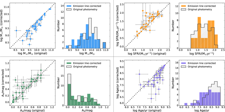
Figure 2. At each quadrant, a pair of panels shows the comparison of outputs from SED fitting with and without the corrections for strong emission-line contributions to the broadband fluxes (left) and the distribution of each SED parameter (right). Hatched and color-filled histograms show those derived based on photometry with and without the correction for emission-line contributions, respectively. The following parameters are shown: top left: stellar masses; top right: SFR; bottom left: attenuation at V band, AV; bottom right: age since the onset of star formation.
Download figure:
Standard image High-resolution imageFigure 3 shows the difference in the best-fit parameters as a function of the fraction of emission-line fluxes in the K band. Stellar mass and age show decreasing trends in the difference with increasing emission-line contributions. SFRs are also affected by large emission-line contributions, but the trend appears weaker than those on stellar mass and age. On the other hand, no clear trend can be seen in AV. This can be understood as longer-wavelength bands are more sensitive to the stellar mass and age, while SFR and dust extinction are primarily captured by the rest-frame UV part of the SED, where emission-line contribution is not important.
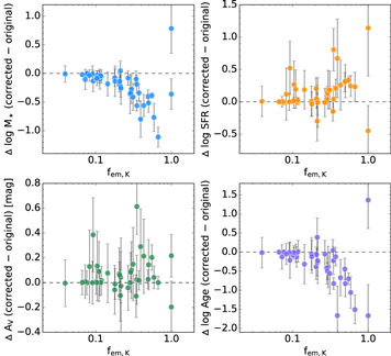
Figure 3. Difference in the best-fit SED fitting parameters (stellar mass, SFR, AV, and age, clockwise from top left panel) between those derived from the original and emission-line-corrected photometry as a function of the fraction of emission-line fluxes in K band.
Download figure:
Standard image High-resolution imageThere are two objects, 434625 and 217090, that have a ∼100% contribution from emission lines in the K band, and they do not seem to follow the general trend of the rest of our sample in Figure 3. These two objects are the only ones without detection both in the K band (after emission-line correction) and in any of the IRAC bands. At z ≃ 3.3, only observing at wavelengths on and beyond the K band can one capture the rest-frame wavelength of >4000 Å, which is essential to properly estimating the mass-to-light ratios of galaxies. This is likely the main reason why the two objects do not follow the trends, especially in stellar mass and age.
All this indicates the importance of a proper assessment of emission-line contribution in near-infrared bands at z > 3 (e.g., Schaerer et al. 2013; Stark et al. 2013). In the following analysis, we adopt  for the stellar masses of galaxies in our sample.
3.4. UV Slope and Dust Extinction
We computed the UV spectral slope  defined as
  by fitting a linear function to the observed broadband magnitudes from the r to the J band, which cover the rest-frame wavelength range 1400 ≲ λ ≲ 2800 Å at z = 3.27. We used the rest-frame wavelengths corresponding to the Galaxy Evolution Explorer (GALEX) far-UV (FUV; λc ≃ 1530 Å) and near-UV (NUV; λc ≃ 2300 Å) bands to derive βUV photometrically, following the recipe used in Pannella et al. (2015). For all objects in the sample, this choice of passbands encloses the rest-frame UV wavelengths with which UV slopes are determined. Following Nordon et al. (2013), magnitude errors are further weighted by
  , where λfilter and λFUV are the rest-frame central wavelengths of each photometric band and that of GALEX FUV. By using the best-fit relation,
  was derived as

where mFUV and mNUV are the AB magnitudes in the GALEX FUV and NUV bands, respectively (Nordon et al. 2013; Pannella et al. 2015). Then assuming the Calzetti extinction law (Calzetti et al. 2000; Pannella et al. 2015),  was converted to dust attenuation at λ = 1530 Å with

which assumes an intrinsic (un-extincted) slope  (AV = 0) = −2.10 (Calzetti et al. 2000).
In Figure 4, the values of AV from UV and SED fitting are compared, having converted AUV to AV by assuming the Calzetti extinction law as shown in Table 3. There appears to be no tight correlation between the two estimates, perhaps because dust extinction degenerates with other parameters such as SFH and age in broadband SED fitting (e.g., Kodama et al. 1999; Michałowski et al. 2014). Two outliers, 214339 and 211934, as indicated in Figure 4, turn out to be the faintest galaxies in our sample. Indeed, the broadband SED of these objects shown in Section  difficult.
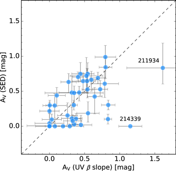
Figure 4. Comparison of the attenuation at V band estimated from SED fitting with that converted from  derived with UV β slope and the Calzetti extinction law. Dashed lines correspond to the one-to-one relation.
Download figure:
Standard image High-resolution imageFigure 5 shows AUV versus stellar mass. There is a trend with more massive galaxies being more dust attenuated. The sample of z ≃ 3.4 SFGs from Troncoso et al. (2014) is also shown, with on average a higher dust extinction compared to our sample. Note that in their study extinction was derived from broadband SED fitting, while ours was based on  slope. Troncoso et al. (2014) specifically selected Lyman break galaxies (LBGs) with redshifts from near-IR spectroscopy, while we selected objects partly based on the availability of spectroscopic redshifts, which automatically puts a limit on BAB = 25 mag for those galaxies culled from the zCOSMOS-Deep sample. Moreover, targets were selected based on the predicted
  flux of >5 × 10⁻¹⁸ erg s−1 cm−2. Though this flux limit does not seem to be too high, the combination of these two criteria could result in selecting bluer, less dust-attenuated objects compared to the standard LBG selection employed by Troncoso et al. (2014).

Figure 5. AUV vs. stellar mass. Our sample is shown with blue circles, and those taken from Troncoso et al. (2014) are shown with green squares. UV attenuation for Troncoso et al. (2014) is converted from  from broadband SED fitting by assuming the Calzetti law.
Download figure:
Standard image High-resolution imageAnother noticeable feature of Figure 4 is that there is an appreciable number of objects (∼20%) showing AV close or equal to zero, which seems somewhat at odds with the relatively high SFR of galaxies in our sample. The adopted calibration of the  –AUV relation in Equation (3) was established at z = 0, but the relation could be different at high redshift for a number of reasons, such as different intrinsic β slope owing to stellar population properties, IMF, SFH (e.g., Reddy et al. 2010; Wilkins et al. 2011), or a different extinction curve than the one assumed here (e.g., Reddy et al. 2015). Castellano et al. (2014) investigated the UV dust extinction for a sample of LBGs at z ≃ 3, obtaining an intrinsic slope of
  = −2.67, which is significantly steeper than widely used values of
  = −2.10 (Calzetti et al. 2000) and
  = −2.23 (Meurer et al. 1999). Indeed, for our galaxies with AV close or equal to zero the measured
  is close to or slightly steeper than −2.10, either because of measurement errors or because the intrinsic slope is actually steeper than −2.10.
3.5. Star Formation Rate
In this section, we derive SFR based on UV and Hβ luminosities. The resulting SFRs are listed in Table 3.
3.5.1. UV Luminosity
We adopt the calibration of the UV luminosity-based SFR from Daddi et al. (2004) after converting from Salpeter IMF to Chabrier IMF by applying an offset of 0.23 dex:

where LUV,corr is extinction-corrected UV luminosity derived using

Here the UV luminosity is measured at rest-frame 1500 Å.
In the left panel of Figure 6, we compare the UV-based SFRs with those from SED fitting, showing that the two measurements agree well with each other.

Figure 6. Comparison of SFR derived by UV luminosity with that derived from broadband SED fitting (left) and  (right).
  SFRs are corrected for dust extinction from UV β slope and assuming
  . Dashed lines show the one-to-one relation.
Download figure:
Standard image High-resolution imageFigure 7 shows SFR as a function of stellar mass for z ≃ 3.3 SFGs. Our sample covers about 2.5 dex in stellar mass from  to ≃11, essentially following the MS at z = 3.27 derived by Speagle et al. (2014), which also traces the parent sample of z ≃ 3.3 SFGs shown with gray scale. We also derived the best-fit relation between stellar mass and SFR for our sample, finding
shown with the solid line. Because of the sample selection based either on the availability of spectroscopic redshift or on the predicted  flux, our sample is likely to be biased against especially low mass and low SFR galaxies. We believe that this is the main reason why we obtained a flatter MS slope compared to that of the parent sample and that of the Speagle et al. (2014) MS. We will use Equation (6) only to separate the sample into bins of M⋆ and sSFR to create composite spectra (see Section 3.6).
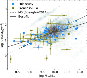
Figure 7. SFR–stellar mass relation for galaxies at 3 < z < 3.8. Blue circles show the UV-based SFR of our sample, and background pixels show SFR from SED fitting of photo-z selected galaxies at 3 < z < 3.8 (Ilbert et al. 2013). Green squares are galaxies at 3 < z < 5 by Troncoso et al. (2014). SFRs of their objects are estimated from  luminosity. The dashed line indicates the star-forming MS at z = 3.27 (Speagle et al. 2014).
Download figure:
Standard image High-resolution imageFor comparison, overplotted in Figure 7 is the sample of z ≃ 3.4 SFGs from Troncoso et al. (2014). Their sample shows an even flatter slope than ours. Again, this could be due to their sample selection based on the LBG technique, which prefers galaxies with blue SEDs and shows a flat SFR–stellar mass relation (e.g., Erb et al. 2006b). Note that their SFRs are based on  luminosity with extinction correction assuming an extra extinction in the nebular component, i.e.,
  , while UV-based SFRs are used for our sample. Thus, both our best-fit and Troncoso et al. (2014) distributions appear to be flatter than the canonical MS (Speagle et al. 2014), which can result from a bias favoring low-mass SFGs with above average sSFR and disfavoring high-mass galaxies with high dust extinction. Relatively low dust extinction is indeed obtained for our sample in the analysis above. In particular, we might miss high-metallicity objects owing to this possible bias, if the correlation between metallicity and dust extinction claimed at an intermediate redshift z ≃ 1.6 (Zahid et al. 2014) still holds at z ∼ 3.3.
3.5.2. Hβ Luminosity
We converted  luminosities to the
  luminosities, assuming an intrinsic
  /
/ ratio of 2.86 (Case B recombination with T = 104 K and ne = 102 cm−3; Osterbrock & Ferland 2006). Then the SFR based on
  was computed following Kennicutt & Evans (2012),

For the objects in which  is not detected with more than 3σ, we adopted 3σ upper limits.
In the original recipe by Calzetti et al. (2000), calibrated with local UV-luminous starbursts, nebular emission lines are attenuated more than stellar light following  . However, there have been various claims in recent years indicating that at high redshift these two components may suffer similar attenuations (e.g., Erb et al. 2006b; Kashino et al. 2013; Pannella et al. 2015; Puglisi et al. 2016). Therefore, we assumed the same amount of attenuation for the stellar light as for emission lines, which actually provides a good agreement between UV-based and
  -based SFRs as shown in the left panel of Figure 6.
In addition to the relation between nebular emission lines and stellar continuum extinction, there is an uncertainty in the choice of the extinction curve for nebular emission lines. Related to the original derivation of the Calzetti et al. (2000) relation, the Milky Way extinction curve (Cardelli et al. 1989) or Small Magellanic Cloud (SMC) extinction curve (Gordon et al. 2003) is often preferred (e.g., Steidel et al. 2014). In the estimate of  -based SFRs we use the Calzetti et al. (2000) extinction curve. Note that for our range of AV, the change between Calzetti et al. (2000) and Cardelli et al. (1989) extinction curves is very minor: at most 2% for the
  flux and 0.03 dex for log([O iii]/[O ii] λ3727).
3.6. Composite Spectra
In the next sections we will compare various properties of the ionized gas with global properties of galaxies, such as stellar mass, SFR, and sSFR. Besides carrying out such a comparison for individual galaxies, we will also compare average properties. For this purpose, we created composite spectra in bins of stellar mass and SFR. The sample, excluding the two AGN candidates, was split into three bins in stellar mass, log M/M⊙ < 9.5, 9.5 < log M/M⊙ < 10.0, and log M/M⊙ > 10.0, and two bins in SFR, above and below the best-fit MS shown as the dashed line in Figure 7, i.e., ΔMS < 0 and ΔMS > 0, where ΔMS ≡ sSFR/sSFRbest-fit.
First, spectra of each object in both J and H band were normalized by total [O iii] λ5007 flux and registered by a linear interpolation to the rest-frame wavelength grid of the 0.25 Å interval, which is slightly finer than the spectral resolution for the highest-redshift object of our sample. We also normalized the corresponding noise spectra by total [O iii] λ5007 flux and registered to the identical rest-frame wavelength grid but interpolated in quadrature. Then composite spectra were constructed by taking an average at each wavelength pixel weighted by the inverse variance. We constructed the associated noise spectra via the standard error propagation from the individual noise spectra.
Emission-line fluxes are measured by fitting a Gaussian to each emission line by assuming a common velocity shift and a velocity dispersion. We fit simultaneously [O ii] λλ3726, 3729,  , [O iii] λλ4959, 5007, and [Ne iii] λ3869, with continuum described by a second-order polynomial. We computed the flux values and their 1σ errors by means of a Monte Carlo simulation with 103 realizations.
The resulting stacked spectra are shown in Figure 8. We adopt median stellar mass, SFR, and AV whenever they are used in the subsequent analysis (see Table 4).
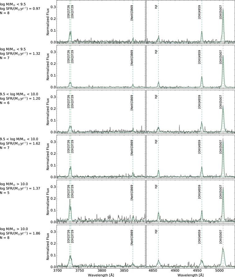
Figure 8. Composite spectra in bins of stellar mass and SFR above and below the best-fit "main sequence" (Figure 7). The range of stellar mass, median SFR, and number of objects stacked in each bin is indicated at each row. The panels show the observed composite spectra (black) with associated 1σ noise (gray) and the best-fit Gaussians for the emission lines (green). For each mass bin, the upper/lower panels show the composite spectra of galaxies below/above the adopted MS.
Download figure:
Standard image High-resolution imageTable 4. Properties of Stacked Spectra
| Nobj | log M⋆ | log SFR | AV | log q | log ne |

|
|---|---|---|---|---|---|---|
| (M⋆/M⊙) | (M⊙ yr−1) | (mag) | (cm s−1) | (cm−3) | ||
| (1) | (2) | (3) | (4) | (5) | (6) | (7) |
| Above the Best-fit MS | ||||||
| 8 | 9.26 | 0.97 | 0.20 |

|

|

|
| 6 | 9.82 | 1.20 | 0.34 |

|

|

|
| 5 | 10.29 | 1.37 | 0.35 |

|

|

|
| Below the Best-fit MS | ||||||
| 7 | 9.13 | 1.32 | 0.28 |

|

|

|
| 7 | 9.66 | 1.62 | 0.55 |

|

|

|
| 8 | 10.34 | 1.86 | 0.76 |

|

|

|
Note. (1) Number of objects in the bin; (2) median stellar mass; (3) median SFR; (4) median AV; (5) ionization parameter; (6) electron density; (7) gas-phase oxygen abundance.
Download table as: ASCIITypeset image
4. MEASUREMENTS OF IONIZED GAS PROPRIETIES
In this section, we derive physical properties of ionized gas, namely, gas-phase oxygen abundance, ionization parameter, and electron density, of our sample. The obtained values are listed in Tables 4 and 5 for the stacked spectra and individual objects, respectively.
Table 5. Ionizing Gas Properties
| ID | log q | log ne |

|
|---|---|---|---|
| (cm s−1) | (cm−3) | ||
| 434625 |

|
⋯ |

|
| 413136 | >7.42 | ⋯ | ⋯ |
| 413646 | >7.40 | ⋯ | ⋯ |
| 413453 | ⋯ | ⋯ | ⋯ |
| 434585 |

|
>3.23 |

|
| 434571 | >7.50 | ⋯ | ⋯ |
| 413391 |

|

|

|
| 427122 | >7.50 | ⋯ | ⋯ |
| 434148 |

|
⋯ |

|
| 434082 |

|

|

|
| 434126 |

|

|

|
| 434139 | >7.49 | ⋯ | ⋯ |
| 434145 |

|
⋯ |

|
| 434242 |

|
<2.51 |

|
| 406390 |

|
>2.90 |

|
| 406444 |

|
<2.77 |

|
| 434227 | >7.87 | ⋯ | ⋯ |
| 191932 |

|

|

|
| 434547 |

|

|

|
| 192129 |

|

|

|
| 193914 |

|
⋯ |

|
| 212863 |

|

|

|
| 195044 |

|
⋯ |

|
| 208115 | ⋯ | ⋯ | ⋯ |
| 200355 |

|
⋯ |

|
| 214339 |

|

|

|
| 411078 |

|

|

|
| 212298 |

|
⋯ |

|
| 412808 |

|
⋯ |

|
| 223954 |

|

|

|
| 220771 |

|

|

|
| 219315 |

|

|

|
| 434618 |

|

|

|
| 221039 |

|

|

|
| 215511 |

|

|

|
| 217597 |

|

|

|
| 211934 |

|
⋯ |

|
| 434579 |

|
<2.78 |

|
| 217753 |

|

|

|
| 218783 |

|
⋯ |

|
| 217090 |

|

|

|
| 210037 |

|

|

|
| 208681 |

|

|

|
A machine-readable version of the table is available.
Download table as: DataTypeset image
4.1. Gas-phase Oxygen Abundance
The primary indicator for gas-phase metallicity,  , in this study is R23 ≡ ([O ii] λ3726 + [O ii] λ3729 + [O iii] λ4959 + [O iii] λ5007)/
 (Pagel et al. 1979; Kobulnicky & Phillips 2003). For the metallicity measurement, we adopt the empirical calibration by Maiolino et al. (2008), in which the low-metallicity regime (
 ≲ 8.3) is directly calibrated by the electron temperature method. At this metallicity scale, the theoretical calibration has been known to have difficulties in reproducing the observed emission-line ratios (e.g., Kewley & Dopita 2002). This appears to still exist in the recent photoionization models by Dopita et al. (2013), as shown in Figure 9, i.e., calibration lines by Maiolino et al. (2008) show higher ratios at low metallicity than those from Dopita et al. (2013). The line ratios from the stacked spectra (Figure 8) are shown as hexagon symbols in Figure 9, clearly showing that at low metallicities the photoionization models by Dopita et al. (2013) cannot account for all five line ratios simultaneously.

Figure 9. Best-fit metallicity vs. observed line ratios for our sample. Diamonds show objects with detected [O ii] λλ3726, 3729, [O iii], and [Ne iii] λ3869, while circles are those with detected [O ii] λλ3726, 3729 and [O iii]. Filled and open symbols show those with and without  detection, respectively. In the case of undetected
  , its flux is supplemented from UV SFR. The orange open pentagon shows the values obtained from the stacking of all non-AGN objects. Solid lines are photoionization models by Dopita et al. (2013), with κ = 20 for the κ-distribution of electron energies. Gray scale of each line indicates log q = 6.5, 6.75, 7.0, 7.25, 7.5, 7.75, 8.0, 8.25, 8.5 from faint to thick, where q is the ionization parameter, defined as the ratio of the ionizing photon flux passing through a unit area and the local number density of hydrogen atoms. Dashed lines show an empirical calibration by Maiolino et al. (2008) that we adopted in this study. The bottom left panel is a histogram of
  .
.
Download figure:
Standard image High-resolution imageFor our metallicity estimates, following Maiolino et al. (2008), we used the five extinction-corrected line ratios shown in Figure 9, namely, R23, [O iii] λ5007/ , [O iii] λ5007/[O ii] λλ3726, 3729, [O ii] λλ3726, 3729/
 , and [Ne iii] λ3869/[O ii] λλ3726, 3729, for the metallicity estimate. For the stacked spectra, we corrected for dust extinction with the median AV derived from the
  slope.
For the metallicity analysis of individual galaxies we removed seven objects without 3σ detection in [O ii] λ3726 + [O ii] λ3729 and the two AGN candidates (one of two is also [O ii] λ3727 nondetection). This leaves us with 35 objects. In the case that either [O iii] λ4959 or [O iii] λ5007 is undetected at the 3σ level, the other [O iii] flux is complemented by assuming an intrinsic line ratio of [O iii] λ5007/[O iii] λ4959 = 3. For eight objects without >3σ  detection, we used the
  flux estimated from the UV-based SFR, given the relatively tight correlation between the SFRs from the two estimators as shown in Figure 6. [Ne iii] λ3869 is detected for 10 out of the 35 objects.
The gas-phase oxygen metallicity was then derived with the maximum likelihood method, first computing
where  and
and  are the ith line ratio from Maiolino et al. (2008) calibration at a given
  and the one from observed spectra. Further,
  and
and  are the errors in the observed line ratio and intrinsic scatter measured as in Jones et al. (2015) for z = 0.8 galaxies. Then, we translated χ2 to the likelihood distribution using
  . The metallicity and its confidence interval are then defined as the median and the 16th–84th percentiles of the probability distribution, respectively.
Note that the Maiolino et al. (2008) calibration adopted in this study implicitly assumes the ionization parameter at a given metallicity to be independent of redshift, as it is derived for local SFGs. Recent studies of gas-phase metallicity of high-redshift SFGs show an offset in the BPT diagram with higher [O iii]/ ratio at a given [N ii]/
 ratio, which can be ascribed either to an elevated ionization parameters in high-redshift galaxies (e.g., Kewley et al. 2013) or to an enhanced N/O abundance ratio at a fixed O/H ratio (e.g., Cullen et al. 2014; Masters et al. 2014; Nakajima & Ouchi 2014; Yabe et al. 2015; Sanders et al. 2016). Moreover, Sanders et al. (2016) have argued that there is no significant change in ionization parameter at a fixed metallicity from z ∼ 0 to z ∼ 2.3. Unfortunately, the [N ii] λ6583/
 ratio that is used to break the degeneracy of metallicity estimates from R23 cannot be obtained from the ground for the redshift of our galaxies, but will become possible with the James Webb Space Telescope. Maier et al. (2015) suggest that the [O iii] λ5007/Hβ ratio can be used to break the degeneracy, with galaxies with log [O iii] λ5007/
 > 0.26 having
  < 8.6 on the Kewley & Dopita (2002) metallicity scale. Indeed, our sample with
  < 8.6 always has log [O iii] λ5007/
 > 0.26, confirming the Maier et al. (2015) result.
4.2. Ionization Parameter
The ionization parameter, q, is defined as  , where
  is the flux of ionizing photons above the Lyman limit, Rs is the Strömgren radius, and n is the local number density of hydrogen atoms (e.g., Kewley & Dopita 2002). The ionization parameter can be derived through a q-sensitive line ratio, O32 ≡ [O iii] λλ4959, 5007/[O ii] λλ3726, 3729 (e.g., McGaugh 1991). Here we adopt a metallicity-dependent [O iii]/[O ii]–q relation of Kewley & Dopita (2002) parameterized by Kobulnicky & Kewley (2004) as
where y = log O32. The results are reported in Table 5.
Note that the ionization parameters derived in this way are not fully self-consistent, as we used the Maiolino et al. (2008) calibration for gas-phase metallicity (see Section 4.1), which implicitly assumed ionization parameters of normal star-forming galaxies in the local universe. Note also that in this and the following analysis all emission-line fluxes have been corrected for dust extinction using E(B − V)star derived based on  slope by assuming the Calzetti extinction curve and
  .
.
4.3. Electron Density
The relatively high spectral resolution of MOSFIRE allows us to resolve the [O ii] λλ3726, 3729 doublet as seen in individual spectra. The ratio of the two [O ii] lines is sensitive to electron density (Osterbrock & Ferland 2006), and we used the PyNeb 15 package (Luridiana et al. 2015) to compute the electron density ne of the line-emitting regions of our galaxies. We assumed an electron temperature of Te = 104 K. At low to intermediate redshift, Te is indeed observed to be ∼(1–2) × 104 K via the direct measurements of the [O iii] λ4363 line (e.g., Izotov et al. 2006; Nagao et al. 2006; Andrews & Martini 2013; Ly et al. 2014; Jones et al. 2015). Assuming a higher Te, e.g., 2 × 10⁴ K, the resulting ne will become systematically higher by ∼0.15 dex.
When one of the [O ii] lines is not detected at the 3σ level, either upper or lower limits of ne are derived from the 3σ flux limit of the line. In the case that both of the [O ii] lines are detected, we have carried out a Monte Carlo simulation with 500 realizations by perturbing the measured line ratios with the associated 1σ uncertainties. The median and 16th and 84th percentiles of the resulting distribution have been taken as ne and 1σ confidence interval, respectively.
5. DISCUSSION
5.1. Relation between Ionized Gas and Galaxy Properties
Figure 10 shows the relation between R23 and O32. The local, z ≃ 0 galaxy sample shown in the background was selected from the OSSY catalog (Oh et al. 2011) as star-forming based on the BPT diagram (Baldwin et al. 1991; Kewley et al. 2006) by requiring all four emission lines ( , [O iii] λ5007,
  , and [N ii] λ6583), as well as [O ii] λ3727 with S/N > 3. The higher line ratios of z ∼ 3.3 galaxies relative to the local SFGs indicate that our galaxies have a higher ionization parameter, on average (Nakajima & Ouchi 2014; Shirazi et al. 2014). Our z = 3.3 galaxies lie along the tail of the local distribution and extend it to higher log R23 and log O32 values, typical of SFGs at z = 2–3 (e.g., Henry et al. 2013; Nakajima & Ouchi 2014; Sanders et al. 2016). Locally, the tail of the distribution consists of metal-poor galaxies, typically with
  ≲ 8.5. Since the majority of our sample also shows
  ≲ 8.5 (See Section 4.1), we argue that the ionization parameter could be similar at a given metallicity in both low- and high-redshift galaxies, consistent with Sanders et al. (2016).

Figure 10. O32 vs. R23. Individual galaxies from our sample are shown with blue circles, with filled and open ones corresponding to those with and without  detection, respectively.
  fluxes of objects without
  detection are estimated from UV-based SFR. For the stacked data shown with orange squares, open and filled squares represent ΔMS < 0 and ΔMS > 0, respectively, with the size proportional to the median stellar mass of each bin. Since error bars for the stacked points are smaller than the size of the symbols, they are not shown here. Background pixels show the distribution of local SFGs selected based on the BPT diagram drawn from the Sloan Digital Sky Survey line measurement catalog of Oh et al. (2011).
Download figure:
Standard image High-resolution imageFigure 11 compares various galaxy physical quantities with the ionization parameter. The strong correlation between log q and  is trivial, as both
  and log q strongly depend on [O iii]/[O ii]. Among the other parameters shown in Figure 11, we do not find significant correlations between any of them, with the exception of the SFR–log q plot. The Spearman's correlation coefficient between SFR and log q is −0.35, corresponding to a two-sided p-value of 0.04, when considering objects without an upper or lower limit in log q. A similar but more significant correlation between SFR and O32 is found by Sanders et al. (2016) for z ∼ 2.3 SFGs, with a two-sided p-value of 0.002. This correlation can be understood as a result of a correlation between SFR and metallicity and an anticorrelation between ionization parameter and metallicity (Pérez-Montero 2014; but see Dors et al. 2011). Nakajima & Ouchi (2014) and Sanders et al. (2016) found correlations of O32 with stellar mass and sSFR, as well as with SFR. While we do not see such correlations for individual objects, stacked data points show some hints of a similar correlation for log q with stellar mass and sSFR.

Figure 11. Comparison of the ionization parameter of our sample with (a) stellar mass, (b) SFR, (c) sSFR, (d) ΔMS ≡ sSFR/sSFRMS, and (e) gas-phase oxygen abundance  . Symbols are the same as in Figure 10.
Download figure:
Standard image High-resolution imageIn Figure 12 we also compare various physical parameters with the electron density measured from the line ratio of the [O ii] λλ3726, 3729 doublet. The measured electron densities of ∼100–1000 cm−3 are about one order of magnitude higher than those of typical SFGs at z = 0, roughly consistent with those reported for other high-redshift galaxies (e.g., Masters et al. 2014; Shirazi et al. 2014; Shimakawa et al. 2015; Sanders et al. 2016). In Figure 12 there is no indication of strong correlations in any of the parameters with the electron density, which is also confirmed by the very low Spearman's rank correlation coefficients, indicating less than 1σ significance, for individual objects and for stacked points.

Figure 12. Comparison of the electron density of our sample with (a) stellar mass, (b) SFR, (c) sSFR, (d) ΔMS ≡ sSFR/sSFRMS, (e) gas-phase oxygen abundance  , and (f) ionization parameter log q. Symbols are the same as in Figure 10.
Download figure:
Standard image High-resolution imageShimakawa et al. (2015) measured the electron density of a sample of  narrowband-selected SFGs at z = 2.5 through the resolved [O ii] λ3727 doublet. They found a positive correlation with a 4σ significance between ne and sSFR. However, from panel (c) of Figure 12, the correlation between sSFR and ne does not seem to be strong in our sample. If at all, there is a hint for an opposite trend with higher-sSFR galaxies with lower ne. Based on a larger sample at z ∼ 2.3, Sanders et al. (2016) also do not find any correlation of electron density with stellar mass, SFR, or sSFR.
5.2. [O ii] Luminosity as an SFR Indicator
The [O ii] λ3727 emission line luminosity has been used as an indicator of SFR (e.g., Kennicutt 1998), though it depends not only on SFR but also on metallicity and ionized gas properties. Figure 13 shows the relation between the [O ii] luminosity and the UV-based SFR. Here, both quantities were extinction corrected using UV-based estimates and assuming  as before. The [O ii] luminosities of our sample do not seem to follow the calibration of SFR([O ii]) by Kewley et al. (2004), shown as the dashed line in Figure 13. We derived the best-fit calibration of [O ii] λ3727 SFR for our z ≳ 3 MS galaxies as

having fixed the slope to unity. Our best fit gives 0.22 dex lower SFRs compared to the Kewley et al. (2004) calibration. If the extinction toward the H ii region were higher, like the original Calzetti law, i.e.,  , then the discrepancy would become more prominent.
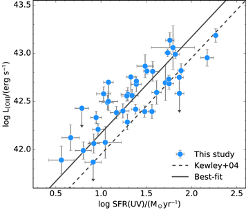
Figure 13. [O ii] λ3727 luminosity vs. UV-based SFR. The solid line shows the best-fit linear regression with a slope of unity computed by using LTS_LINEFIT (Cappellari et al. 2013). The dashed line corresponds to Equation (4) in Kewley et al. (2004) converted from Salpeter to Chabrier IMF.
Download figure:
Standard image High-resolution imageThe elevated [O ii] luminosity relative to the local relation could be due to a change in the physical condition of star-forming regions as discussed above, i.e., higher ionization parameter and electron density in high-redshift galaxies.
5.3. Mass–Metallicity Relation
Figure 14 shows the MZR for our galaxies, both individually and for the stacked spectra, in comparison with the MZRs at lower redshifts. The MZRs at z = 0.07, 0.7, and 2.2 are from Tremonti et al. (2004), Savaglio et al. (2005), and Erb et al. (2006a), respectively, converted to the same metallicity calibration, and parameterized by Maiolino et al. (2008). We also plot the MZR at z ≃ 3.4 from Troncoso et al. (2014) and that at z = 0 taken from Mannucci et al. (2010). The majority of our sample follows the previously defined MZR at z ≃ 3.4, i.e., our MZR offsets by ≃0.7 dex and ≃0.3 dex from those at z ≃ 0 and z ≃ 2, respectively. There are, however, a few objects showing higher metallicity, by up to 0.3–0.4 dex compared to the stack points. Owing to a small sample size especially at M⋆ > 1010.5 M⊙, we do not attempt to constrain the turnover mass of MZR here. Instead, we carried out a linear regression and found the best-fit MZR for the individual objects in our sample as
as shown in the left panel of Figure 14 with a dashed line.

Figure 14. Left: mass–metallicity relation of our sample, shown with circles. The filled and open circles are those with and without  detection, respectively. Squares represent the measurements on the stacked spectra in bins of stellar mass and SFR. The bins above and below the best-fit MS are shown with filled and open symbols, respectively. The best-fit linear relation for our sample is shown with a dashed line. The solid line is the z = 0 relation (Mannucci et al. 2010). Right: our z ∼ 3.3 stacked data points (orange squares) shown in the left panel are compared with MZR at various redshifts. Solid lines are taken from Maiolino et al. (2008) for z = 0.07, 0.72, and 2.2 relations by Tremonti et al. (2004), Savaglio et al. (2005), and Erb et al. (2006a), respectively. Dotted and dot-dashed lines are mass–metallicity relations from Troncoso et al. (2014) defined based on the measurement on the stacked spectra and the average of individual objects, respectively. Two filled regions are predictions at z = 3.3 by a gas-regulation model by Lilly et al. (2013) shown in the left panel. In both panels, orange and green shaded areas are predictions from a gas-regulator model (Lilly et al. 2013) fixing the star formation efficiency ε to the locally calibrated value and allowing ε to increase as
  . The areas enclose the case for 0 < Z0/y < 0.1.
Download figure:
Standard image High-resolution imageIn Figure 14 we plot ranges between minimum and maximum stellar masses in each bin as error bars for the stack points. The metallicities from the stacked spectra appear to be lower than the average or median of the individual measurements at a given stellar mass bin. This may be due to the way they were employed for stacking: we normalized each spectrum by the total [O iii] λ5007 flux and then stacked with weights proportional to the inverse variance. This procedure gives more weights for [O iii] bright objects, which tend to have lower metallicities. Indeed, as shown in Figure 23 in Appendix  compared with those presented above. However, our conclusion does not depend on the choice of the stacking method since our analysis on the metallicity is based mainly on individual objects.
Figure 15 shows that there appears to be no correlation between  and SFR relative to the distances from the best-fit MZR and MS within the error bars for both stacked and individual points, respectively. A similar behavior has been reported for z ∼ 2 SFGs (Steidel et al. 2014; Wuyts et al. 2014; Sanders et al. 2015), while Zahid et al. (2014) found an anticorrelation between SFR and metallicity in a sample of SFGs at z ∼ 1.6 (see also Yabe et al. 2015). This suggests that the role of SFR as a second parameter in the MZR may be less important at z ≃ 3.3 compared to that in the local universe (e.g., Mannucci et al. 2010; Andrews & Martini 2013). We shall return to this issue in Section 5.4.
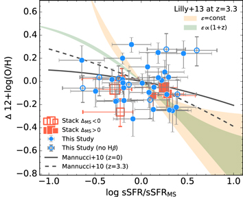
Figure 15. Difference of  from the best-fit linear regression in the MZR for our sample,
  , as a function of ΔMS. Symbols of data points and two filled regions are the same as in Figures 10 and 14, respectively, and solid and dashed lines represent the fundamental
  relation by Mannucci et al. (2010) adjusted to z = 0 and z = 3.3 MS, respectively. Lilly et al. (2013) models and Mannucci et al. (2010) relations are obtained for M = 1010 M⊙ galaxies.
Download figure:
Standard image High-resolution imageThe redshift evolution of metallicity at a stellar mass of 1010 M⊙ is illustrated in the right panel of Figure 16. For the comparison, data points at different redshifts are taken from Tremonti et al. (2004) for z = 0.07, Savaglio et al. (2005) for z = 0.72, and Erb et al. (2006a) for z = 2.2 after being corrected to the same metallicity calibration used here by Maiolino et al. (2008), Troncoso et al. (2014) for z = 3.4, Zahid et al. (2014) for z = 1.55, Henry et al. (2013) for z = 1.7, Cullen et al. (2014) for z = 2.2, Steidel et al. (2014) for z = 2.3, and Sanders et al. (2015) for z = 2.3. Note that all these data are converted to the metallicity calibration of Maiolino et al. (2008), when needed.

Figure 16. Redshift evolution of MZR. Our z ∼ 3.3 data are shown with a filled circle. The data point and error bar indicate the average and standard deviation of the metallicity of the objects with log M⋆/M⊙ = 10 ± 0.2. Open squares are adopted from Table 5 in Maiolino et al. (2008) for z = 0.07, 0.72, and 2.2 relations by Tremonti et al. (2004), Savaglio et al. (2005), and Erb et al. (2006a), respectively. An open square at z = 3.4 is taken from Troncoso et al. (2014). Filled symbols at z < 3 are taken from the following literature: Zahid et al. (2014) for z = 1.55 (hexagon), Henry et al. (2013) for z = 1.7 (square), Cullen et al. (2014) for z = 2.2 (diamond), Steidel et al. (2014) for z = 2.3 (pentagon), and Sanders et al. (2015) for z = 2.3 (triangle). Two filled regions are predictions at z = 3.3 by a gas-regulation model by Lilly et al. (2013) shown in Figure 14.
Download figure:
Standard image High-resolution image5.4. Mass–Metallicity–SFR Relation
Mannucci et al. (2010) found that in the local universe SFGs lie close to a 3D surface in the space with SFR, stellar mass, and metallicity as coordinates (see also Lara-López et al. 2010). They also found that SFGs lie close to the same surface at least to z ≃ 2.5, suggesting the existence of the so-called FMR, and showed that a projection of the surface over the plane with coordinates  and
and  is able to minimize the scatter about the surface itself. Figure 17 shows such a 2D plane, where most of the objects in our sample are offset from the locally defined FMR by ≃0.3 dex.
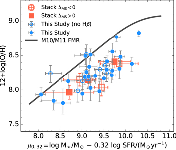
Figure 17. Comparison of gas-phase oxygen abundance with ![${\mu }_{0.32}\equiv \mathrm{log}({M}_{\star }[{M}_{\odot }])-0.32\mathrm{log}(\mathrm{SFR}[{M}_{\odot }\;{\mathrm{yr}}^{-1}])$](https://content.cld.iop.org/journals/0004-637X/822/1/42/revision1/apj523269ieqn384.gif) . The FMR proposed by Mannucci et al. (2010) is shown with the solid line extended to μ0.32 < 9.5 following Mannucci et al. (2011).
. The FMR proposed by Mannucci et al. (2010) is shown with the solid line extended to μ0.32 < 9.5 following Mannucci et al. (2011).
Download figure:
Standard image High-resolution imageComparing the left panel in Figures 14 and 17, it is not obvious whether in the case of our galaxies using μ0.32 as a coordinate reduces the scatter in metallicity in the MZR, as it does locally. We left the α in  as a free parameter and computed the standard deviation around the best-fit linear regression in the
  –μα relation for our sample. The scatter as a function of α is shown in Figure 18. Mannucci et al. (2010) claimed that at z = 0 with α = 0.32 the scatter decreases to ≃0.02 dex compared to ≃0.06 dex in the case of the simple MZR (i.e., α = 0). In contrast, varying α does not seem to reduce the observed scatter around the best-fit line for our z = 3.3 galaxies, but it remains essentially constant around 0.15 dex. We should note that the typical uncertainties of metallicity from strong lines are in general comparable to the scatter in the MZR, in this study and in the literature (e.g., Marino et al. 2013; Steidel et al. 2014), which may explain why by varying α the scatter does not change. Indeed, the number of objects in our sample is still too small to overcome the dominance of the measurement error and to draw firm conclusions on the intrinsic scatter of our z ∼ 3.3 MZR. To push down the sampling error, orders of magnitude larger samples would be required, e.g., ≳105 objects are used in the study of Mannucci et al. (2010) for the local galaxies, whereas z ≳ 2 samples include only ≳101–2 objects.

Figure 18. Standard deviation around the best-fit linear regression in the  –μα relation as a function of α, where
  . The solid line and filled region are the median and 1σ confidence interval, respectively, based on 104 bootstrap resampling.
Download figure:
Standard image High-resolution image5.5. A Comparison with a Simple Gas-regulator Model
Because of the redshift evolution in both the MS and metallicity, our sample spans a parameter space that is not well covered by the local galaxy population (Maier et al. 2014). Therefore, an extrapolation of the  relation is inevitable when trying to compare the local relation with the high-redshift one. A more physically motivated relation among the three parameters,
  , is proposed by Lilly et al. (2013), which indeed can reproduce the FMR at z = 0 and at z ≃ 2.3 with a sensible choice of parameters. We then use the
  relation in Equation (40) in Lilly et al. (2013):
where Zeq is the equilibrium metallicity, Z0 is the metallicity of the incoming gas, y is the chemical yield, λ is the mass-loading factor (≡ outflow rate/SFR), R is the fraction of mass return due to stellar evolution, ε is the star formation efficiency (SFE ≡ SFR/Mgas), β is the MS slope defined as  , and t is the age of the universe in units of Gyr. In Lilly et al. (2013) λ and ε are parameterized as follows:


where m10 is the stellar mass in units of 1010 M⊙.
Following Lilly et al. (2013), we fix the ε and λ parameters to the values that reproduce the local FMR of Mannucci et al. (2010), and then we use Equation (12) to derive the MZR at z = 3.3 predicted by this regulator model. The result is shown in Figure 14, with the orange shaded area encompassing the cases between Z0/y = 0 and Z0/y = 0.1.
Observations suggest that the SFE may be higher at higher redshift (e.g., Daddi et al. 2010; Genzel et al. 2010). We also show with the green shaded area in Figure 14 the model predictions in the case for  . These two cases virtually enclose our z ≃ 3.3 sample, while the majority of them are consistent with the prediction with nonevolving ε.
In Section 5.4 we have shown that the scatter of the MZR does not change appreciably by introducing the SFR as a second parameter. Together with the observed data, Figure 15 shows the corresponding relations as predicted by the regulator models, as well as those observationally defined and extrapolated for the MS at z = 3.3. In general, compared to our data, a steeper dependence is predicted for the metallicity offset from the MZR as a function of the SFR offset from the MS. Although this apparent mismatch may be due to large errors and small sample size, it may give some insight into the functional form of the SFH of the galaxies studied here. Indeed, the dependence of metallicity on SFR would disappear if galaxies were evolving at constant SFR, i.e.,  (see Appendix
In Figure 16 we compare the redshift evolution of the MZR at M⋆ = 1010 M⊙ with the model predictions described above. The evolving  relation assuming ε ∝ (1 + z) traces the observed trend up to z ≃ 2.5, with an exception for the data point of Cullen et al. (2014). As mentioned above, our sample appears to prefer a nonevolving star formation efficiency, as do the data by Maier et al. (2014) at z ∼ 2.3. However, the observational scatter of ≳0.1 dex for the high-redshift measurements may hamper us from distinguishing models at better than the ≃2.5σ level. On the other hand, the departure in metallicity from the original z = 0 FMR by Mannucci et al. (2010), as seen in Figure 17, can be due to the extrapolation of the local FMR into a parameter space that is basically unpopulated at z = 0. Perhaps a more suitable γ would lie in between the two cases above, 0 and 1. For instance, a recent study by Genzel et al. (2015) derived γ = 0.34 ± 0.15, based on a combined analysis of CO and dust scaling relations at 0 ≲ z ≲ 3. Of course, the other parameters of the regulator model and their mass dependence may also evolve with redshift, hence being different at z ≃ 3.3, but the current sample size is too small to explore the entire parameter space.
6. SUMMARY
Using the rest-frame optical spectra of 43 normal star-forming galaxies lying close to the star-forming MS at z ∼ 3.3, we carried out a study of the properties of the ionized gas and their relations with global galaxy parameters. Our main results can be summarized as follows.
- 1.Strong optical emission lines contribute significantly to the broadband flux, especially in the K band, with a median of 21%, but up to ∼100% in a few cases. These emission lines affect the estimate of stellar masses from SED fitting by 0.13 dex (median), but the difference may exceed ∼0.5 dex when the emission-line contribution is ≳40%.
- 2.A comparison between UV- and
 -based SFRs suggests a lower additional extinction toward H ii regions at z ∼ 3.3, compared to the local calibration (Calzetti et al. 2000).
 - 3.The ionization parameter appears to be systematically higher than its average for the local SFGs, extending the local relationship in the R23 versus O32 diagram. The ionization parameter derived from the O32 indices does not show any correlation with galaxy global properties, except with the SFR. However, the correlation between SFR and ionization parameter for our sample is not very significant (≃2σ) compared with those in the literature (e.g., Sanders et al. 2016). Electron density derived from resolved [O ii] λ3727 doublets also does not show any correlation with galaxy properties.
- 4.The MZR of our z ∼ 3.3 galaxies shows a ∼0.7 dex offset from the local relation and a ∼0.3 dex offset relative to z ∼ 2, indicating very rapid evolution of gas-phase metallicity at z ∼ 3.
- 5.Among our galaxies at z ≃ 3.3 we do not find any correlation of metallicity with SFR. If such a correlation exists, it has to span a metallicity range narrower than measurement errors.
- 6.Our z ∼ 3.3 sample does not follow the locally defined FMR, with metallicities being offset by ∼0.3 dex compared to the value predicted by the FMR for z = 3.3. This mismatch may result from the extrapolation of the relation empirically defined at z = 0 to Z, SFR, and M⋆ combinations that are not well populated by z = 0 galaxies, hence giving an incorrect prediction for the evolution of MZR.
- 7.For our sample, no projection of the relation to the μα space is able to reduce the scatter in metallicity, suggesting that the SFR may not play a significant role as a second parameter in the MZR. However, the uncertainties in metallicity determination and the small sample size prevent us from drawing a firm conclusion on this issue.
- 8.A comparison of the MZR of our galaxies and those at different redshifts with the prediction of a simple gas-regulator model suggests that a weakly evolving star formation efficiency could better account for the observed redshift evolution of MZR.


The data presented herein were obtained at the W. M. Keck Observatory, which is operated as a scientific partnership among the California Institute of Technology, the University of California, and the National Aeronautics and Space Administration. The Observatory was made possible by the generous financial support of the W. M. Keck Foundation. The authors wish to recognize and acknowledge the very significant cultural role and reverence that the summit of Mauna Kea has always had within the indigenous Hawaiian community. We are most fortunate to have the opportunity to conduct observations from this mountain. The observations were partly carried out within the framework of the Subaru–Keck time exchange program. This research made use of Astropy, 16 a community-developed core Python package for Astronomy (Astropy Collaboration et al. 2013), APLpy, 17 an open-source plotting package for Python, and matplotlib, 18 a Python 2D plotting library (Hunter 2007). We thank Scott Dahm, Marc Kassis, Jim Lyke, Greg Wirth, and the rest of the staff at the Keck Observatory for supporting the observations; Andreas Faisst, Nicholas Konidaris, Luca Rizzi, and Benny Trakhtenbrot for the assistance on the MOSFIRE data reduction; and Roberto Maiolino, Claudia Scarlata, and Maryam Shirazi for insightful discussions. We thank the anonymous referee for providing constructive comments. A.R. is grateful to the Institute for Astronomy at ETH Zurich for its kind hospitality while working on this project.
Facility: Keck I (MOSFIRE).
APPENDIX A: MOSFIRE SPECTRA
Figure 19 presents the 1D and 2D MOSFIRE spectra of individual objects. The best-fit combination of Gaussians for each emission line ([O ii] λλ3726, 3729, [Ne iii] λ3869, Hβ, and [O iii] λλ4959, 5007) is overplotted.

Figure 19.
MOSFIRE spectra of each object in H (left) and K band (right). Top: 2D spectra. Bottom: 1D spectra for objects (solid line), 1σ noise (gray filled area), and the best fit (green solid line). From left to right, dashed lines indicate the location of [O ii] λλ3726, 3729, [Ne iii] λ3869,  , and [O iii] λλ4959, 5007.
(The complete figure set (43 images) is available.)
, and [O iii] λλ4959, 5007.
(The complete figure set (43 images) is available.)
Download figure:
Standard image High-resolution imageAPPENDIX B: HUBBLE SPACE TELESCOPE (HST) IMAGE STAMPS
Figure 20 shows HST Advance Camera for Surveys (ACS) F814W stamps of those with robust spectroscopic redshifts. For those observed with the CANDELS and 3D-HST surveys (Grogin et al. 2011; Koekemoer et al. 2011; Brammer et al. 2012; Skelton et al. 2014), ACS F606W, Wide Field Camera 3 (WFC3) F125W, F140W, and F160W images are shown in Figure 21.
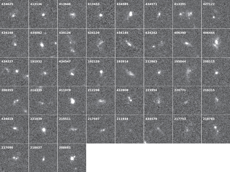
Figure 20. HST/ACS F814W stamps of the sample. North is up, and the size of each stamp is 3 × 3 arcsec2.
Download figure:
Standard image High-resolution image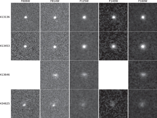
Figure 21. HST CANDELS stamps of the sample. North is up, and the size of each stamp is 3 × 3 arcsec2. The ACS/F814W image is the same as in Figure 20, and the WFC3/F140W image is from 3D-HST.
Download figure:
Standard image High-resolution imageAPPENDIX C: BROADBAND SED
Figure 22 shows the broadband photometry and best-fit SEDs of individual objects in our sample. Downward arrows indicate 5σ upper limits.
APPENDIX D: WHO DOES CONTRIBUTE THE MOST IN THE STACKING?
Figure 9 shows each line ratio as a function of  and distribution of
  . The stacked spectrum shows lower metallicity than the median metallicity of all objects. The same trend was seen in a previous work by Troncoso et al. (2014), in which they found slightly lower metallicity at a given stellar mass for the stacked measurement than the average of individual measurements. At least in our case, this discrepancy can be explained by the way we stacked spectra. We normalized each spectrum by the [O iii] λ5007 luminosity and stacked them weighted by the inverse variance at each wavelength pixel. Therefore, the resulting emission lines of stacked spectra are dominated by objects with higher S/N and less OH skyline contamination. In Figure 23, we show absolute fluxes and S/N of strong emission lines as a function of gas-phase oxygen abundance for individual galaxies. As seen from the figure, [O iii] is indeed dominated by metal-poor objects, while
  and [O ii] λ3727 emission lines have more contribution from more metal-rich objects. However, in the case that only [O iii] has enhanced flux with respect to the other lines, the line ratios used to investigate the metallicity tend to favor low metallicity, in particular for the [O iii]/[O ii] λ3727 ratio.

Download figure:
Standard image High-resolution image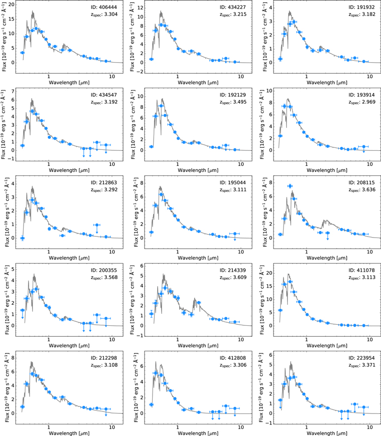
Download figure:
Standard image High-resolution image
Figure 22. Best-fit SED.
Download figure:
Standard image High-resolution image
Figure 23. Left: fluxes of [O ii] λ3727 (top),  (middle), and [O iii] λ4959 (bottom) as a function of gas-phase oxygen abundance. Right: S/Ns for the same emission lines as the left panels as a function of
  . Dashed lines indicate S/N = 3.
Download figure:
Standard image High-resolution image
APPENDIX E: ON THE SFR DEPENDENCE ON METALLICITY IN THE REGULATOR MODEL OF LILLY ET AL. (2013)
The general form of gas-phase metallicity in a quasi-steady state of the gas-regulator model by Lilly et al. (2013) is their Equation (28) as follows:
Since  ,
,  is calculated as
where dM⋆/dt is substituted by  as this term describes the buildup of long-lived stars in the system (see Lilly et al. 2013).
Substituting the denominator of the second term in Equation (15) by Equation (16) yields
Therefore, Equation (15) can be written as
If the SFR of the system is constant, obviously there is no SFR dependence in metallicity as  .
.
Footnotes
- 9
- 10
- 11
- 12
This offset was introduced to convert the photometric zero point in Capak et al. (2007) derived by using spectrophotometric standard stars to that based on sources with a flat spectrum such as moderate-redshift galaxies (Ilbert et al. 2009, 2013; C. Laigle et al. 2016, in preparation). The former zero point suffered from the uncertainty caused by the combination of sharp Balmer absorption features of the calibration stars and the location of the blue edge of the filter, which is sensitive to temperature and humidity, while the latter is less sensitive to exact knowledge of the bandpass.
- 13
- 14
Sum of living stars and remnants.
- 15
- 16
- 17
- 18