


ABSTRACT
We present a census of Lyα emission at  , utilizing deep near-infrared Hubble Space Telescope grism spectroscopy from the first six completed clusters of the Grism Lens-Amplified Survey from Space (GLASS). In 24/159 photometrically selected galaxies we detect emission lines consistent with Lyα in the GLASS spectra. Based on the distribution of signal-to-noise ratios and on simulations, we expect the completeness and the purity of the sample to be 40%–100% and 60%–90%, respectively. For the objects without detected emission lines we show that the observed (not corrected for lensing magnification) 1σ flux limits reach 5 × 10⁻¹⁸ erg s−1 cm−2 per position angle over the full wavelength range of GLASS (0.8–1.7 μm). Based on the conditional probability of Lyα emission measured from the ground at
  , we would have expected 12–18 Lyα emitters. This is consistent with the number of detections, within the uncertainties, confirming the drop in Lyα emission with respect to
  . Deeper follow-up spectroscopy, here exemplified by Keck spectroscopy, is necessary to improve our estimates of completeness and purity and to confirm individual candidates as true Lyα emitters. These candidates include a promising source at z = 8.1. The spatial extent of Lyα in a deep stack of the most convincing Lyα emitters with
  is consistent with that of the rest-frame UV continuum. Extended Lyα emission, if present, has a surface brightness below our detection limit, consistent with the properties of lower-redshift comparison samples. From the stack we estimate upper limits on rest-frame UV emission line ratios and find
  and
and ![${f}_{{\rm{C}}{\rm{III}}]}/{f}_{\mathrm{Ly}\alpha }\lesssim 0.23$](https://content.cld.iop.org/journals/0004-637X/818/1/38/revision1/apj521744ieqn6.gif) , in good agreement with other values published in the literature.
, in good agreement with other values published in the literature.
Export citation and abstract BibTeX RIS
1. INTRODUCTION
With the deployment of the Wide Field Camera 3 (WFC3) on the Hubble Space Telescope (HST) in 2009, the samples of galaxies at the epoch of reionization, the phase transition from a completely neutral intergalactic medium (IGM) to a fully ionized IGM at  , have grown dramatically. One of the main results of the WFC3 imaging campaigns has been the accurate determination of the luminosity function of star-forming high-redshift (based on their photometry) Lyman break galaxies (e.g., Bouwens et al. 2015b; Finkelstein et al. 2015b). The UV luminosity functions of Lyman break galaxies have provided key constraints on the physics of reionization (e.g., Robertson et al. 2013; Duffy et al. 2014; Schmidt et al. 2014b). For example, it is clear that the population of galaxies that has been detected so far cannot produce enough hard photons to keep the universe ionized. However, the luminosity function is found to have a steep faint-end slope (approximately
  ). Thus, faint galaxies could in principle provide enough ionizing photons (Barone-Nugent et al. 2015; Bouwens et al. 2015a; Dressler et al. 2015; Robertson et al. 2015), even though a contribution from active galactic nuclei might end up being necessary (Giallongo et al. 2015; Madau & Haardt 2015).
Ground-based spectroscopic follow-up of photometrically selected high-redshift candidates has also been an important part of these studies and has provided additional clues about the reionization epoch. Remarkably, only a handful of sources have been confirmed above redshift 7 (Vanzella et al. 2011; Ono et al. 2012; Schenker et al. 2012, 2014; Finkelstein et al. 2013; Oesch et al. 2015; Roberts-Borsani et al. 2015; Zitrin et al. 2015b). The low probability of detecting Lyα in Lyman break galaxies could be interpreted as the result of an increased optical depth in the IGM due to a significant fraction of neutral hydrogen. Thus, the decline in detected Lyα is potentially a "smoking gun" of reionization (Fontana et al. 2010). The conditional probability of Lyα emission for Lyman break galaxies is potentially a powerful probe of the physics of the intergalactic and circumgalactic media and their neutral fraction at these redshifts (Dijkstra et al. 2011; Jensen et al. 2013; Dijkstra 2014; Mesinger et al. 2015), provided that large enough spectroscopic samples can be gathered (Treu et al. 2012, 2013; Pentericci et al. 2014; Tilvi et al. 2014).
Currently, progress is limited by the available near-infrared (NIR) spectroscopy at  and the paucity of sources with confirmed Lyα emission at
  . Many efforts are under way to increase the spectroscopic samples (Vanzella et al. 2009, 2014a, 2014b; Pentericci et al. 2011, 2014; Bradač et al. 2012; Caruana et al. 2012, 2014; Treu et al. 2012, 2013; Balestra et al. 2013; Faisst et al. 2014; Karman et al. 2014; Schenker et al. 2014; Tilvi et al. 2014; Hoag et al. 2015; Oesch et al. 2015; Watson et al. 2015; Zitrin et al. 2015b), although progress from the ground is fundamentally limited by the Earth's atmosphere.
In this paper, we report on a spectroscopic study of 159 photometrically selected galaxies at  in the first six fields targeted by the Grism Lens-Amplified Survey from Space (GLASS; P.I. T. Treu; Schmidt et al. 2014a; Treu et al. 2015). By combining HST's NIR slitless spectroscopic capabilities with the power of the gravitational magnification by foreground massive galaxy clusters, we carry out the largest survey of Lyα emission at
  to date. We reach 1σ line sensitivities of order 5 × 10⁻¹⁸ erg s−1 cm−2 over the wavelength range 0.8–1.7 μm, uninterrupted by sky emission or absorption. Including the lensing magnification, μ, of the individual sources, these sensitivities improve by a factor of μ, to intrinsic depths that are unreachable without the lensing of the foreground clusters. Hence, as will become clear in the following, GLASS is providing a unique view of the intrinsically fainter emitters, complementary to the bright spectroscopically confirmed Lyα emitters recently presented by Oesch et al. (2015), Roberts-Borsani et al. (2015), and Zitrin et al. (2015b). We introduce human-based and automated procedures to identify and quantify the significance of the lines and estimate the purity and completeness of the sample. After correcting our statistics for incompleteness and impurity, we compare them with predictions of simple phenomenological models of the Lyα emission evolution. We stack the detections to obtain the first constraint on the spatial distribution of Lyα at these redshifts, as well as limits on the Lyα/C iv and Lyα/C iii] line ratios.
The paper is organized as follows. In Section 2 we briefly summarize the GLASS data set. In Section 3 we introduce our photometric selections and the GLASS grism spectroscopy of sources at  . In Sections 4–6 we describe the measurement of flux and equivalent widths of the features identified as Lyα and estimate the sample completeness and purity. In Section 7 we describe a few interesting cases in detail and discuss the implications these could lead to in Section 8. In Sections 9 and 10 we stack the most convincing line emitters to look for C iv and C iii] emission, estimate the spatial extent of Lyα at
  , and compare it with simulated
  galaxies from the Lyα reference sample (LARS) sample, before we conclude our study in Section 11.
AB magnitudes (Oke 1974; Oke & Gunn 1983) and a standard concordance cosmology with  ,
,  , and h = 0.7 are adopted throughout the paper.
2. THE GLASS DATA AND DATA REDUCTION
GLASS is a 140-orbit slitless spectroscopic survey with HST observing 10 massive galaxy clusters, including the six Hubble Frontier Fields clusters (HFF; P.I. J. Lotz) and eight of the CLASH clusters (P.I. M. Postman; Postman et al. 2012). Taking advantage of the gravitational lensing of the GLASS clusters, the GLASS grism spectroscopy reaches flux limits of background sources otherwise unreachable with the same exposure time. An overview of GLASS and its science drivers is given in the first paper of this series (Treu et al. 2015). One of the key science drivers of GLASS is to study how and when galaxies reionized the universe, taking advantage of this lens-improved depth and emission-line detection limit. Here we present the first results of this study.
As part of GLASS the core of each cluster has been observed using the HST NIR WFC3 G102 and G141 grisms. Each grism exposure is accompanied by a shallower direct image exposure in F105W or F140W to optimize alignment and extraction of the reduced grism spectroscopy. The GLASS observations are split into two distinct position angles (PAs) roughly 90° apart. This is done to minimize the number of objects severely affected by contaminating flux from neighboring objects and to improve the identification of emission lines. The GLASS data were taken following the observing strategy of the 3D-HST survey. The images and spectra are reduced using an updated version of the 3D-HST pipeline (Brammer et al. 2012; Momcheva et al. 2015). The individual grism exposures are aligned and combined using the AstroDrizzle software from the DrizzlePac (Gonzaga et al. 2012) and tweakreg. The grism backgrounds are subtracted using sky images from Kümmel et al. (2011) and Brammer et al. (2012). The direct images are sky-subtracted by fitting a second-order polynomial to the background. After alignment and sky subtraction, the final mosaics are interlaced to a grid of roughly  Å pixel–1 for the G102 (G141) grisms. Before sky subtraction and interlacing the individual exposures were checked and corrected for backgrounds affected by the helium Earth glow described by Brammer et al. (2014) (see Treu et al. 2015, for details).
The individual spectra of objects detected by SExtractor (Bertin & Arnouts 1996) in the direct detection image mosaics are then extracted from the grism mosaics, using the information about the grism dispersion properties provided in the grism configuration files. Flux contamination from neighboring objects is taken into account when extracting the spectra. For the current study, we generated direct image segmentation maps using combined NIR mosaics, including the ancillary CLASH imaging, for source detection and alignment. Note that in this way, by predicting the location of the spectral traces from the grism configuration files based on a detection in the ancillary detection images, it is possible to extract spectra for objects (just) outside the grism field of view.
For further information on GLASS we refer the reader to Schmidt et al. (2014a), Treu et al. (2015), and http://glass.astro.ucla.edu.
3. SAMPLE SELECTION AND SPECTROSCOPY
The sample of high-redshift galaxies analyzed in this study is selected behind the first six completed GLASS clusters Abell 2744, MACS J0717.5+3745, MACS J1423.8+2404, MACS J2129.4–0741, RXC J1347.5–1145, and RXC J2248.7–4431. We make use of HFF images for A2744, the first HFF cluster with complete GLASS and HFF coverage. The remainder of the GLASS/HFF sample will be analyzed and published after the completion of the HFF imaging campaign. In Figure 1 the color images of these six clusters are shown with the two 90° separated GLASS pointings indicated by the magenta polygons. In the following we describe the photometric preselection of the spectroscopic samples shown by the colored circles in Figure 1.
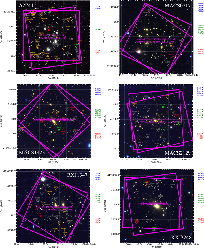
Figure 1. False-color composite images of the six GLASS clusters analyzed in this paper. From top left to bottom right we show Abell 2744, MACS J0717.5+3745, MACS J1423.8+2404, MACS J2129.4–0741, RXC J1347.5–1145, and RXC J2248.7–4431. Next to each panel the individual images used to generate the blue, green, and red channels of the color composites are listed. The magenta polygons mark the field of view of the two 90° separated GLASS pointings. The circles mark the location of the  objects described in Section 3. The orange and gray circles mark the "Gold" and "Silver" objects from Table 2. The green and red circles show the location of the "Gold_EL" and "Silver_EL" objects presented in Table 3. The redshift distributions of these sources are shown in Figure 3. Note that objects immediately outside the GLASS field of view (MACS J1423.8+2404 in the center left panel) can still be recovered and extracted in the grism observations thanks to their detection in the ancillary CLASH imaging. The apparent overdensity of high-redshift objects in Abell 2744 (top left) is caused by the increased depth (compared to the CLASH imaging) of the completed HFF data on Abell 2744. A similar improvement in sample size is expected for the remaining five HFF clusters in the GLASS sample.
Download figure:
Standard image High-resolution image3.1. Preselection of Spectroscopic Sample
We assembled an extensive list of Lyman break galaxy candidates at  , including both existing samples published in the literature and photometric samples selected through multiple color selections and photometric redshift estimates using the ancillary (NIR-based) CLASH photometry. The applied selections and literature samples considered are as follows:
- 1.The Lyman break galaxies at
 investigated by Zheng et al. (2014).
 - 2.The dropouts and multiple-imaged sources presented by Ishigaki et al. (2015).
- 3.
- 4-8.F814W-, F850LP-, F105W-, F110W-, and F125W-dropouts, selected using the color criteria presented by Huang et al. (2015). The selections use HST photometry only. A small subset of candidates have IRAC detections that support the photometric redshift solutions at. See Huang et al. (2015) for details.
- 9.The components of the geometrically supported redshift 10 candidate multiply imaged system presented by Zitrin et al. (2014)
- 10.The candidate presented by Laporte et al. (2014).
- 11.The multiply imaged systems from Lam et al. (2014) above z = 6.5, i.e., systems 17 and 18.
- 12.High-redshift candidates from Huang, Hoag, and Bradač selected as part of follow-up efforts carried out with DEIMOS and MOSFIRE on Keck.
- 13-14.z- and Y-band dropouts following Bouwens et al. (2011), where bands blueward of the z/Y band were required to have S/N.
- 15.z-band dropouts selected following Bouwens et al. (2012). Again, bands blueward of the z band were all required to have S/N.
- 16.
- 17.
- 18.Galaxies with photometric redshifts estimated with the photometric redshift code EAzY (Brammer et al. 2008) run on the CLASH photometry of the CLASH clusters in the sample (all but Abell 2744).
- 19.The CLASH spectral energy distribution selected Lyman break galaxies from Bradley et al. (2014).
- 20-21.Conservative photometric selections based on the CLASH F850LP, F110W, F125W, and F160W photometry. All objects from the photometric selections were visually inspected to weed out contaminants and secure clean nondetections in bands blueward of F850LP.


To summarize, selections 1–3, 9–11, and 19 are all taken from the literature. The images of all objects passing the color and spectral energy distribution selections applied to the ancillary photometry by our team (selections 4–8, 12–18, and 20–21) were visually inspected to remove hot pixels, diffraction spikes, and edge defects from the samples. We have tabulated this summary in Table 1.
Table 1. Summary of Photometric Preselections of Spectroscopic Sample
| Cluster | Selection: | Selection: | N
|
|---|---|---|---|
| GLASS Team | Literature | ||
| A2744 | 4, 5, 6, 7, 8 | 1, 2, 3, 9, 10, 11 | 11 |
| MACS0717 | 4, 5, 6, 7, 8, 12, 13, 14, 15, 16, 17, 18 | 19 | 13 |
| MACS1423 | 4, 5, 6, 7, 8, 13, 14, 15, 16, 17, 18 | ... | 11 |
| MACS2129 | 4, 5, 6, 7, 8, 13, 14, 15, 16, 17, 18 | 19 | 12 |
| RXJ1347 | 4, 5, 6, 7, 8, 13, 14, 15, 16, 17, 18, 20, 21 | 19 | 14 |
| RXJ2248 | 4, 5, 6, 7, 8, 13, 14, 15, 16, 17, 18 | 19 | 12 |
Download table as: ASCIITypeset image
We split the photometric samples into a "Gold" and "Silver" sample according to the number of times each object was selected. Our Gold sample consists of objects picked up by two or more of the above selections. The Gold and Silver samples were furthermore split into an emission-line ("EL") and non-emission-line sample, as described in Section 3.3.
The apparent overdensity of high-redshift objects in Abell 2744 seen in Figure 1 is caused by the increased depth of the HFF imaging on Abell 2744 compared to the CLASH mosaics, and the extra attention on Abell 2744 this has caused. A similar improvement in sample size is expected for the remaining five HFF clusters in the GLASS sample, when their completed HFF photometry is available. We will present these samples in a future publication, when all HFF data will be available on the GLASS clusters.
The final samples of objects are listed in Tables 2 and 3. The "N ," "Sel.," and
  " columns list the number of selections finding a given object out of the total N selections from Table 1, which selections include the object and the mean redshift of the selection(s), respectively. The "Sample" column lists what sample the objects belong to.
Table 2.
 Dropout Samples with No Lyα Detection from Visual Inspections
| Cluster | ID | ID | R.A. | decl. | P.A. | Sample | N /N /N
|
Sel. |

|
F140W |

|
μ |
|---|---|---|---|---|---|---|---|---|---|---|---|---|
| GLASS | Ancillary | (degree) | (degree) | (degree) | (ABmag) | (1e-17 erg s−1 cm−2) | ||||||
| A2744 | 00085 | 03230 | 3.593803625 | −30.415444323 | 135, 233 | Gold | 4/11 | 2, 3, 4 | 6.55 | 26.08 ± 0.05 | ... | 3.7 ± 1.8 |
| A2744 | 00131 | 03158 | 3.570658150 | −30.414663281 | 135, 233 | Gold | 3/11 | 2, 3, 4 | 6.25 | 26.62 ± 0.07 | ... | 1.6 ± 0.4 |
| A2744 | 00220 | 03040 | 3.592948356 | −30.413331741 | 135, 233 | Gold | 2/11 | 2, 3 | 5.96 | 27.74 ± 0.08 | 0.94 | 6.6 ± 4.1 |
| A2744 | 00307 | 02873 | 3.585805956 | −30.411751960 | 135, 233 | Gold | 2/11 | 2, 3 | 7.25 | 26.61 ± 0.04 | 0.48 | 3.8 ± 1.5 |
| A2744 |
 a
a
|
02721 | 3.603208705 | −30.410356491 | 135, 233 | Gold | 4/11 | 1, 2, 3, 4 | 6.5 | 27.08 ± 0.05 | 0.54 | 3.7 ± 7.5 |
| A2744 | 00412 | 02732 | 3.600611950 | −30.410302069 | 135, 233 | Gold | 3/11 | 2, 3, 4 | 6.40 | 28.29 ± 0.19 | 0.57 | 9.2 ± 3.4 |
| A2744 |
 a
a
|
02676 | 3.592367074 | −30.409889954 | 135, 233 | Gold | 4/11 | 1, 2, 3, 11 | 7.39 | 28.86 ± 0.12 | 0.35 | 7.0 ± 7.1 |
| A2744 | 00458 | 02627 | 3.604762132 | −30.409290304 | 135, 233 | Gold | 2/11 | 3, 4 | 6.53 | 27.80 ± 0.07 | 0.52 | 2.9 ± 8.5 |
| A2744 | 00483 | 02686 | 3.596557317 | −30.409003929 | 135, 233 | Gold | 2/11 | 2, 3 | 7.25 | 27.13 ± 0.07 | 0.36 | 5.0 ± 3.4 |
| A2744 | 00748 | 02234 | 3.580452097 | −30.405043370 | 135, 233 | Gold | 3/11 | 2, 3, 11 | 6.96 | 26.94 ± 0.06 | 0.40 | 5.6 ± 1.1 |
| A2744 | 00807 | 02178 | 3.600055342 | −30.404393062 | 135, 233 | Gold | 2/11 | 2, 3 | 7 | 27.18 ± 0.07 | 0.39 | 4.8 ± 3.4 |
| A2744 | 00818 | 02135 | 3.601100197 | −30.403956945 | 135, 233 | Gold | 3/11 | 2, 3, 4 | 6.25 | 27.90 ± 0.07 | 0.66 | 3.5 ± 1.4 |
| A2744 | 01036 | 01942 | 3.567777944 | −30.401277987 | 135, 233 | Gold | 2/11 | 3, 4 | 6.46 | 27.39 ± 0.16 | 0.56 | 2.1 ± 0.9 |
| A2744 | 01069 | 01891 | 3.601044487 | −30.400590602 | 135, 233 | Gold | 2/11 | 1, 3 | 7.45 | 27.00 ± 0.06 | 0.34 | 2.8 ± 0.8 |
| A2744 |
 b
b
|
−00088 | 3.585323923 | −30.397960001 | 135, 233 | Gold | 3/11 | 2, 3, 11 | 6.90 | 27.16 ± 0.07b | 0.44 | 3.2 ± 2.8 |
| A2744 |
 a
a
|
01506 | 3.597814977 | −30.395957621 | 135, 233 | Gold | 3/11 | 2, 3, 11 | 7 | 26.58 ± 0.04 | 0.39 | 2.9 ± 0.9 |
| A2744 | 01929 | 00847 | 3.606221824 | −30.386645344 | 135, 233 | Gold | 2/11 | 2, 3 | 5.80 | 25.98 ± 0.03 | 1.13 | 1.7 ± 0.7 |
| A2744 | 01972 | 00816 | 3.576890999 | −30.386328547 | 135, 233 | Gold | 3/11 | 2, 3, 4 | 6.44 | 28.22 ± 0.11 | 0.57 | 4.4 ± 7.6 |
| A2744 |
 a
a
|
00765 | 3.596089446 | −30.385830967 | 135, 233 | Gold | 4/11 | 2, 1, 3, 6 | 8 | 26.54 ± 0.04 | 0.30 | 2.5 ± 5.6 |
| A2744 | 02040 | 00723 | 3.608995192 | −30.385282140 | 135, 233 | Gold | 3/11 | 2, 3, 4 | 6.10 | 27.97 ± 0.21 | 1.61 | 1.5 ± 1.0 |
| A2744 | 02157 | 00557 | 3.603418234 | −30.383215863 | 135, 233 | Gold | 3/11 | 2, 3, 4 | 5.80 | 27.69 ± 0.09 | 1.16 | 1.7 ± 0.9 |
| A2744 | 02193 | 00477 | 3.603853194 | −30.382264279 | 135, 233 | Gold | 3/11 | 1, 2, 3 | 8.40 | 26.91 ± 0.04 | 0.44 | 1.6 ± 0.9 |
| A2744 |
 a
a
|
00469 | 3.603383290 | −30.382256248 | 135, 233 | Gold | 4/11 | 1, 2, 3, 6 | 8.10 | 25.82 ± 0.04 | 0.44 | 1.6 ± 0.9 |
| A2744 | 02204 | 00479 | 3.604003006 | −30.382306486 | 135, 233 | Gold | 2/11 | 1, 2 | 8.10 | 27.74 ± 0.07 | 0.44 | 1.6 ± 0.9 |
| A2744 | 02209 | 00487 | 3.598091105 | −30.382391542 | 135, 233 | Gold | 2/11 | 1, 3 | 7.64 | 27.79 ± 0.16 | 0.31 | 1.8 ± 2.3 |
| A2744 | 02266 | 00433 | 3.605063809 | −30.381462296 | 135, 233 | Gold | 3/11 | 1, 2, 3 | 7.70 | 27.99 ± 0.14 | 0.47 | 1.5 ± 0.8 |
| A2744 |
 a
a
|
00600 | 3.606467680 | −30.380994116 | 135, 233 | Gold | 4/11 | 1, 2, 3, 6 | 7.80 | 27.09 ± 0.04 | 0.45 | 1.5 ± 1.0 |
| A2744 | 02295 | 00599 | 3.606564953 | −30.380917190 | 135, 233 | Gold | 3/11 | 1, 2, 3 | 7.60 | 27.07 ± 0.04 | 0.46 | 1.5 ± 1.0 |
| A2744 | 02317 | 00333 | 3.604519959 | −30.380466741 | 135, 233 | Gold | 5/11 | 1, 2, 3, 6, 10 | 8 | 25.86 ± 0.04 | 0.44 | 1.5 ± 0.8 |
| A2744 | 02379 | 00265 | 3.590532446 | −30.379764602 | 135, 233 | Gold | 2/11 | 2, 3 | 6.10 | 27.97 ± 0.10 | 0.76 | 2.2 ± 1.6 |
| A2744 | 02428 | 00163 | 3.588984152 | −30.378668677 | 135, 233 | Gold | 3/11 | 1, 2, 3 | 7.89 | 27.87 ± 0.07 | 0.44 | 2.1 ± 1.6 |
| MACS0717 | 00908 | 01656 | 109.377446020 | 37.743640029 | 020, 280 | Gold | 2/13 | 12, 15 | 7.25 | 27.25 ± 0.19 | 0.44 | 8.5 ± 19.3 |
| MACS1423 | 00684 | 01408 | 215.972592500 | 24.072659477 | 008, 088 | Gold | 3/11 | 13, 15, 17 | 7 | 27.27 ± 0.19 | 0.52 | ... |
| MACS1423 | 01479 | 00656 | 215.928811200 | 24.083905686 | 008, 088 | Gold | 3/12 | 11, 15, 17 | 7 | 26.14 ± 0.11 | 0.68 | ... |
| MACS2129 | 01555 | 00475 | 322.373418740 | −7.680549573 | 050, 328 | Gold | 2/12 | 13, 15 | 7 | 27.87 ± 0.27 | 0.44 | ... |
| MACS2129 | 01792 | 00218 | 322.350848970 | −7.675244331 | 050, 328 | Gold | 2/12 | 18, 19 | 6.85 | 27.25 ± 0.19 | 0.12 | ... |
| RXJ1347 | 00091 | 02025 | 206.876076960 | −11.772996916 | 203, 283 | Gold | 2/14 | 18, 19 | 6.82 | 27.70 ± 0.26 | 0.78 | ... |
| RXJ1347 | 00149 | 01954 | 206.882922680 | −11.770563897 | 203, 283 | Gold | 2/14 | 5, 21 | 7 | 26.18 ± 0.11 | 0.45 | ... |
| RXJ1347 | 00162 | 01951 | 206.877358800 | −11.770481642 | 203, 283 | Gold | 3/14 | 13, 15, 20 | 7 | 28.33 ± 0.39 | 0.27 | ... |
| RXJ1347 | 00301 | 01777 | 206.880670900 | −11.765976036 | 203, 283 | Gold | 2/14 | 13, 15 | 7 | 26.42 ± 0.14 | 0.46 | ... |
| RXJ1347 | 00781 | 01316 | 206.876976150 | −11.757678122 | 203, 283 | Gold | 4/14 | 14, 17, 18, 19 | 7.5 | 26.97 ± 0.16 | 0.38 | ... |
| RXJ1347 |
 c
c
|
01046 | 206.900859670 | −11.754209621 | 203, 283 | Gold | 4/14 | 5, 18, 19, 21 | 7 | 26.09 ± 0.09 | 0.43 | ... |
| RXJ1347 | 01146 | 00943 | 206.891246090 | −11.752606761 | 203, 283 | Gold | 4/14 | 6, 19, 20, 21 | 7.5 | 26.38 ± 0.12 | 0.38 | ... |
| RXJ1347 | 01591 | 00471 | 206.887118070 | −11.745016973 | 203, 283 | Gold | 2/14 | 20, 21 | 7 | 25.65 ± 0.07 | 0.44 | ... |
| RXJ1347 | 01708 | 00346 | 206.882316460 | −11.742182707 | 203, 283 | Gold | 5/14 | 13, 15, 17, 19, 20 | 7 | 26.59 ± 0.13 | 0.45 | ... |
| RXJ1347 | 01745 | 00310 | 206.876001920 | −11.741194080 | 203, 283 | Gold | 3/14 | 18, 19, 20 | 7 | 26.98 ± 0.17 | 0.44 | ... |
| RXJ2248 | 01906 | 00253 | 342.193691160 | −44.516422494 | 053, 133 | Gold | 2/12 | 14, 17 | 8 | 27.60 ± 0.25 | 0.47 | 5.5 ± 3.0 |
| A2744 | 00431 | 02609 | 3.593576781 | −30.409700762 | 135, 233 | Silver | 1/11 | 3 | 6.75 | 26.78 ± 0.04 | 0.46 | 5.3 ± 1.9 |
| A2744 | 00795 | 02186 | 3.576122532 | −30.404490552 | 135, 233 | Silver | 1/11 | 3 | 6.75 | 26.61 ± 0.05 | 0.48 | 3.5 ± 2.0 |
Notes. The "Cluster" column lists the cluster the objects were found in. "ID GLASS" designates the ID of the object in the GLASS detection catalogs. Note that these IDs are not identical to the IDs of the v001 data releases available at https://archive.stsci.edu/prepds/glass/ presented by Treu et al. (2015), as a more aggressive detection threshold and de-blending scheme was used for the current study. "ID Ancillary" lists the IDs from the ancillary A2744 HFF+GLASS and CLASH IR-based photometric catalogs. "R.A." and "decl." list the J2000 coordinates of each object. "P.A." lists the position angle of the two GLASS orientations (the PA_V3 keyword of image fits header). The "Sample" column indicates what sample the object belongs to. "N /N
/N " lists the number of photometric selections picking out each object and the total number of selections applied to the data set from Table 1. The actual selections listed in the "Sel." column are described in Section 3. The
  column lists the median redshift of the
  selections containing the object. "F140W" lists the AB magnitude of the objects. The
  column quotes the line flux limit for the emission lines obtained as described in Section 4. The μ column gives the magnifications of the HFF clusters obtained as described in Section 4. The complete Silver sample is available upon request.
 by Zitrin et al. (2015a) as described in the text.
bObject had no good counterpart (
by Zitrin et al. (2015a) as described in the text.
bObject had no good counterpart ( ) in the default photometric catalog, so its magnitude comes from a more aggressive (with respect to de-blending and detection threshold) rerun of SExtractor.
cRXJ1347_01037 has a confirmed redshift from the GLASS spectra and from Keck DEIMOS as described in Section 7.1. Its GLASS spectra are shown in Figure 6.
) in the default photometric catalog, so its magnitude comes from a more aggressive (with respect to de-blending and detection threshold) rerun of SExtractor.
cRXJ1347_01037 has a confirmed redshift from the GLASS spectra and from Keck DEIMOS as described in Section 7.1. Its GLASS spectra are shown in Figure 6.
Table 3.
 Dropout Samples with Lyα Detections from Visual Inspection
| Cluster | ID | ID | R.A. | Decl. | P.A. | Sample | N /N /N
|
Sel. |
 |
F140W |

|
EW
|
 or or 
|
μ |
|---|---|---|---|---|---|---|---|---|---|---|---|---|---|---|
| GLASS | Ancillary | (degree) | (degree) | (degree) | ( ) ) |
(ABmag) | ( ± 50 Å) | (Å) | (1e-17 erg s−1 cm−2) | |||||
| A2744 | 00463 | 02720 | 3.604573038 | −30.409357092 | 135, 233 | Gold_EL | 3/11 | 2, 3, 4 | 6.1 (6.73) | 28.19 ± 0.13 | 9395, ... | 379 ± 147, ... | 1.91 ± 0.7, 0.65 | 2.9 ± 7.3 |
| A2744 |
 a
a
|
02111 | 3.570068923 | −30.403715689 | 135, 233 | Gold_EL | 2/11 | 3, 4 | 6.5 (6.34) | 26.85 ± 0.04 | 8929, ... | 152 ± 52, ... | 2.76 ± 0.94, 0.88 | 2.0 ± 0.8 |
| MACS1423 | 00648 | 01418 | 215.945534620 | 24.072435174 | 008, 088 | Gold_EL | 3/11 | 13, 15, 17 | 7 (6.88) | 26.05 ± 0.09 | 9585, ... | 56 ± 16, ... | 2.0 ± 0.56, 0.71 | ... |
| MACS1423 |
 b
b
|
01022 | 215.935869430 | 24.078415134 | 008, 088 | Gold_EL | 2/11 | 5, 13 | 7 (6.96) | 26.56 ± 0.12 | 9681, ... | 85 ± 30, ... | 1.87 ± 0.63, 1.04 | ... |
| MACS2129 |
 b
b
|
01408 | 322.353239440 | −7.697441500 | 050, 328 | Gold_EL | 4/12 | 13, 15, 17, 19 | 7 (6.88) | 27.17 ± 0.17 | 9582, 9582 | 272 ± 80, 270 ± 70 | 3.45 ± 0.87, 3.42 ± 0.70 | ... |
| MACS2129 |
 c
c
|
01188 | 322.343220360 | −7.693382243 | 050, 328 | Gold_EL | 2/12 | 7, 14 | 8.5 (8.10) | 26.69 ± 0.13 | 11059, 11069 | 44 ± 31, 74 ± 29 | 0.74 ± 0.52, 1.26 ± 0.47 | ... |
| MACS2129 | 01516 | 00526 | 322.353942530 | −7.681646419 | 050, 328 | Gold_EL | 2/12 | 13, 15 | 7 (6.89) | 28.41 ± 0.33 | 9593, ... | 668 ± 290, ... | 2.7 ± 0.85, 0.58 | ... |
| RXJ2248 | 00207 | 01735 | 342.185601570 | −44.547224418 | 053, 133 | Gold_EL | 2/12 | 13, 15 | 7 (8.55) | 28.61 ± 0.45 | 11609, ... | 920 ± 543, ... | 2.55 ± 1.07, ... | 2.1 ± 0.8 |
| A2744 | 00233 | 03032 | 3.572513845 | −30.413266331 | 135, 233 | Silver_EL | 1/11 | 1 | 8.5 (8.17) | 28.36 ± 0.18 | 11156, ... | 804 ± 338, ... | 2.95 ± 1.14, 0.74 | 1.9 ± 0.4 |
| A2744 | 01610 | 01282 | 3.591507273 | −30.392303082 | 135, 233 | Silver_EL | 1/11 | 4 | 6.5 (5.91) | 27.83 ± 0.07 | ..., 8406 | ..., 355 ± 178 | 1.35, 2.79 ± 1.39 | 8.6 ± 27.0 |
| A2744 | 02273 | 00420 | 3.586488763 | −30.381334667 | 135, 233 | Silver_EL | 1/11 | 3 | 5.71 (6.17) | 28.48 ± 0.12 | 8717, ... | 766 ± 257, ... | 3.21 ± 1.01, 1.02 | 2.7 ± 6.6 |
| MACS0717 | 00370 | 02063 | 109.377007840 | 37.736462661 | 020, 280 | Silver_EL | 1/13 | 14 | 7.5 (6.51) | 27.66 ± 0.28 | 9138, ... | 221 ± 102, ... | 1.87 ± 0.72, 0.43 | 2.5 ± 1.4 |
| MACS1423 | 00435 | 01567 | 215.942403590 | 24.069659639 | 008, 088 | Silver_EL | 1/11 | 18 | 7.27 (7.63 ) | 25.29 ± 0.06 | 10500, ... | 15 ± 7, ... | 1.01 ± 0.47, 0.54 | ... |
| MACS1423 | 00539 | 01526 | 215.932958480 | 24.070875663 | 008, 088 | Silver_EL | 1/11 | 5 | 7 (6.13) | 25.99 ± 0.09 | 8666, ... | 89 ± 29, ... | 3.7 ± 1.17, 0.75 | ... |
| MACS1423 |
 d
d
|
01128 | 215.958132710 | 24.077013896 | 008, 088 | Silver_EL | 1/11 | 14 | 8 (10.27) | 27.81 ± 0.21 | 13702, ... | 558 ± 176, ... | 2.72 ± 0.67, 0.42 | ... |
| MACS1423 | 01169 | 00954 | 215.942112130 | 24.079404012 | 008, 088 | Silver_EL | 1/11 | 6 | 8 (6.99) | 26.01 ± 0.10 | 9721, ... | 62 ± 18, ... | 2.26 ± 0.61, 0.68 | ... |
| MACS1423 | 01412 | 00756 | 215.947908420 | 24.082450925 | 008, 088 | Silver_EL | 1/11 | 15 | 7 (6.77) | 27.84 ± 0.24 | 9448, ... | 190 ± 82, ... | 1.31 ± 0.49, 0.79 | ... |
| MACS1423 | 01619 | 00526 | 215.935606220 | 24.086476168 | 008, 088 | Silver_EL | 1/11 | 5 | 7 (7.17) | 26.53 ± 0.12 | 9932, ... | 59 ± 27, ... | 1.31 ± 0.57, 0.51 | ... |
| MACS2129 | 01182 | 00914 | 322.344533970 | −7.688477035 | 050, 328 | Silver_EL | 1/12 | 14 | 8 (8.99) | 27.64 ± 0.20 | 12145, ... | 606 ± 185, ... | 3.92 ± 0.94, 0.54 | ... |
| RXJ1347 |
 b
b
|
01488 | 206.893075800 | −11.760237310 | 203, 283 | Silver_EL | 1/14 | 13 | 7 (7.84) | 27.85 ± 0.26 | 10750, ... | 290 ± 118, ... | 1.76 ± 0.57, 0.45 | ... |
| RXJ1347 | 00997 | 01070 | 206.895685760 | −11.754637616 | 203, 283 | Silver_EL | 1/14 | 13 | 7 (6.79) | 26.94 ± 0.20 | 9467, 9463 | 149 ± 54, 90 ± 45 | 2.37 ± 0.75, 1.42 ± 0.66 | ... |
| RXJ1347 |
 b
b
|
00864 | 206.899894840 | −11.751082858 | 203, 283 | Silver_EL | 1/14 | 5 | 7 (7.14) | 26.68 ± 0.16 | 9902, ... | 522 ± 87, ... | 10.05 ± 0.84, 0.54 | ... |
| RXJ2248 |
 d
d
|
01561 | 342.201879400 | −44.542663866 | 053, 133 | Silver_EL | 1/12 | 7 | 9 (9.89) | 27.05 ± 0.18 | 13239, ... | 142 ± 64, ... | 1.45 ± 0.61, 0.41 | 1.8 ± 0.5 |
| RXJ2248 | 01953 | 00220 | 342.192399500 | −44.515663484 | 053, 133 | Silver_EL | 1/12 | 14 | 8 (6.50) | 27.99 ± 0.27 | ..., 9118 | ..., 686 ± 227 | 0.95, 4.3 ± 0.94 | 3.8 ± 1.9 |
Notes. The "Cluster" column lists the cluster the objects were found in. "ID GLASS" designates the ID of the object in the GLASS detection catalogs. Note that these IDs are not identical to the IDs of the v001 data releases available at https://archive.stsci.edu/prepds/glass/ presented by Treu et al. (2015), as a more aggressive detection threshold and de-blending scheme was used for the current study. "ID Ancillary" lists the IDs from the ancillary A2744 HFF+GLASS and CLASH IR-based photometric catalogs. "R.A." and "decl." list the J2000 coordinates of each object. "P.A." lists the position angle of the two GLASS orientations (the PA_V3 keyword of image fits header). The "Sample" column indicates what sample the object belongs to. "N /N
/N " lists the number of photometric selections picking out each object and the total number of selections applied to the data set from Table 1. The actual selections listed in the "Sel." column are described in Section 3. The
  column lists the median redshift of the
  selections containing the object, followed by the Lyα redshift for the emission line. "F140W" lists the AB magnitude of the objects. The column
  " lists the wavelength of the detected emission lines. The equivalent width of the Lyα emission lines is given in EW
 .
.  and
and  give the line flux and the flux limit, respectively, for the emission lines obtained as described in Section 4. The μ column gives the magnifications of the HFF clusters obtained as described in Section 4. In columns containing two values separated by a comma, the individual values refer to the corresponding PAs of the GLASS data listed in the column PA.
 source speaks in favor of the object being a contaminating low-redshift line emitter. Spectroscopic follow-up is needed to confirm this.
bObject's G102 grism spectra at the two GLASS PAs are shown in Figure 2.
cThe particularly interesting redshift 8.1 candidate MACS2129_00899 is discussed in detail in Section 7.2.
dAs described in Section 7.3, these two objects are potential low-redshift contaminants.
source speaks in favor of the object being a contaminating low-redshift line emitter. Spectroscopic follow-up is needed to confirm this.
bObject's G102 grism spectra at the two GLASS PAs are shown in Figure 2.
cThe particularly interesting redshift 8.1 candidate MACS2129_00899 is discussed in detail in Section 7.2.
dAs described in Section 7.3, these two objects are potential low-redshift contaminants.
Download table as: ASCIITypeset image
Note that the photometric selections described in this section should not be treated as truly independent selections, as they are all based on essentially the same data, very similar photometry (if not identical), and overlapping selection regions in color space probing the Lyman break, which is also what the photometric redshift selections are sensitive to when searching for high-redshift galaxies.
3.2. Purity and Completeness of Photometric Samples
Photometrically selected samples of high-redshift galaxies are know to be both incomplete and contaminated by low-redshift sources. The incompleteness is usually a consequence of searching for high-redshift galaxies at the detection limits of the imaging data and in the low-S/N regime. Photometric interlopers and contaminants occur as objects mimick the colors of high-redshift galaxies. In particular, the rest-frame 4000 Å break in star-forming galaxies is known to contaminate Lyman break galaxy samples, as the resulting colors from a 4000 Å break are very similar to the ones obtained from a Lyman break. Also, spurious sources and cool dwarf stars are known to mimic the colors of high-redshift galaxies and contaminate Lyman break samples. For detailed discussions on high-redshift galaxy sample contaminants we refer to, e.g., Dunlop (2013), Coe et al. (2013), Wilkins et al. (2014), Finkelstein et al. (2015b), or Bouwens et al. (2015b). As is the case for the completeness of high-redshift samples, the contamination is often a result of lacking depth of the photometry, in particular blueward of the Lyman break, where nondetections are required, as exemplified by a few HST sources by Laporte et al. (2015). Estimated contamination fractions in high-redshift samples range from 10% to over 40% (e.g., Stanway et al. 2003; Malhotra et al. 2005; Schmidt et al. 2014b). As the Silver sample objects were only picked up by one photometric selection, we note that these objects must be considered to have a higher risk of being low-z contaminants. Irrespective of the type and cause of the contamination and lack of completeness, when performing inference using photometrically selected high-redshift galaxy samples, both the contaminants, i.e., the purity, and the completeness need to be properly accounted for. This is often done via visual inspection (to remove contamination from stars and spurious sources) and simulations (e.g., Oesch et al. 2007, 2012; Bouwens et al. 2011). In the present study we focus on the spectroscopic line emitter samples presented in Section 3.3, and the completeness and purity of the photometric preselection therefore do not affect our measurements, given that all the sources have detected line emission. We do have to worry about contamination by low-redshift line emitters, however, As we will describe in Section 7, emission-line galaxy samples are potentially contaminated by, e.g., low-redshift [O ii] λ3727 emitters. Broad wavelength coverage to confirm nondetections of other low-z emission lines and high-resolution spectroscopy to resolve line morphology of individual lines can be used to account for this contamination, as we will show in Section 7.
3.3. Finalizing the Spectroscopic Samples
We extracted the GLASS spectra of all candidates in the Gold and Silver samples detected in the NIR detection image mosaics (see Section 2). Faint photometric candidates from the literature (from high-redshift candidate searches including HFF data on A2744) that were not detected in our NIR mosaics were not extracted and are therefore not included in Tables 2 and 3. As noted, we will present these sources in a future publication.
The extracted GLASS spectra were visually inspected using the publicly available GLASS inspection GUIs GiG and GiGz (see Appendix A of Treu et al. 2015, and https://github.com/kasperschmidt/GLASSinspectionGUIs) by three to four GLASS team members (K.B.S., T.T., M.B., B.V., and L.P.) to identify emission lines. The wavelength of any potential (Lyα) emission was noted and subsequently compared to the other independent inspections. If an emission line was marked by two or more inspectors (within ±50 Å), the object was reinspected by K.B.S. and T.T. The candidates deemed to be real upon reinspection constitute the emission-line sample presented in Table 3. In summary, we have assembled a total of 159 unique high-z galaxies with redshifts  and GLASS spectroscopy in the G102 and G141 grisms. Of these, 55 are found in at least two different preselections (Gold), out of which 8 have emission lines consistent with Lyα (Gold_EL). A total of 104 objects were only selected by one preselection (Silver). Of these, 16 have promising lines consistent with Lyα (Silver_EL). In Figure 2 we show four examples of emission-line objects detected in the GLASS data. Each of the four panels shows the spectra from the two distinct GLASS PAs with the location of the emission line marked by the white circles.

Figure 2. Examples of GLASS spectra for 4 out of the 24  emission-line objects listed in Table 3. For each object the G102 spectrum at both of the GLASS PAs is shown. The assumed Lyα redshift and the selection redshift from Table 3 are quoted above each panel. The circles mark the location of the emission lines. All spectra have subtracted the contamination model had, which comes from the GLASS reduction.
Download figure:
Standard image High-resolution imageAs illustrated by the emission-line wavelengths listed in Table 3, the emission lines were not visually identified in both PAs in the majority of the objects. If the contamination model was perfect, the exposure times were identical and the background level was constant in the data from the two different PAs; the signal-to-noise ratio (S/N) of any detected lines should be the same in the two GLASS spectra. However, given the varying background from the helium Earth glow mentioned in Section 2 (which changes the effective exposure time by up to 13% between PAs), the change in the contribution to the background from the intracluster light in the two dispersion directions, and residuals from subtracting the contamination models (causing larger flux uncertainties and altered background levels), it is not surprising that several of the moderate-S/N line detections are only seen in one PA. We consider objects with lines clearly detected in both PAs, such as MACS2129_00677 shown in Figure 2, to be particularly strong line emitter candidates.
To our knowledge the only spectroscopically confirmed object in our sample of  sources is RXJ1347_01037 at z = 6.76 (Huang et al. 2015), which we will describe in more detail in Section 7.
At redshifts just below 6.5 (and therefore not included in the samples described here) a few objects have been spectroscopically confirmed. In Appendix
The Gold, Gold_EL, Silver, and Silver_EL objects are marked by the orange, green, gray, and red circles, respectively, on each of the color composites shown in Figure 1. The redshift distributions of the samples are shown in Figure 3. Here the mean redshift of the selection(s) is used for the Gold and Silver samples (Table 2), whereas for the Gold_EL and Silver_EL samples (Table 3) we use the redshift corresponding to the emission-line wavelengths listed in the  Å" column.
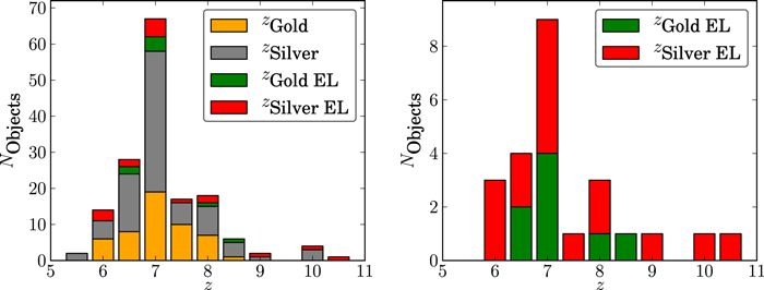
Figure 3. Redshift distribution of the Gold (orange), Silver (gray), Silver_EL (red), and Gold_EL (green) samples from Tables 2 and 3. In both panels, the distributions are stacked to show the total number of sources in each bin. For the Gold and Silver sample the redshift from the photometric selection(s) is used, whereas the redshifts for the EL samples correspond to the redshifts of the emission lines listed in Table 3, assuming that they are Lyα.
Download figure:
Standard image High-resolution image4. FLUX LIMITS AND EQUIVALENT WIDTHS
To quantify the emission-line detections and nondetections, we estimate the line fluxes, emission-line rest-frame equivalent widths, and 1σ line flux sensitivities. The rest-frame equivalent widths, defined by
were estimated based on the extracted two-dimensional spectra. The "integrated" line flux,  , was estimated in two-dimensional ellipsoidal apertures adjusted for each individual object based on the extent of the line and the contamination (subtraction residuals) optimizing S/N and is given by
where  refers to the number of pixels in the ellipsoidal aperture used to enclose the line. For the EL samples,
  has a median size of 66 pixels. The line flux is corrected for background (and contamination) over/undersubtraction, mainly owing to the intracluster light that varies strongly across the field of view, by adjusting the fluxes by the median background flux per pixel in a "background aperture" defined around the emission line for each spectrum,
  . An example of the line and background apertures used for RXJ1347_00627 is shown in Figure 4.
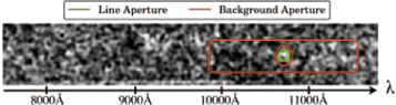
Figure 4. Example of the emission-line and background apertures used when estimating the emission-line fluxes (and 1σ flux sensitivities) of the GLASS spectra of RXJ1347_00627 shown in Figure 2. The line flux is obtained by accumulating ("integrating") the flux in the green ellipsoidal line aperture ( ). The red background aperture (excluding the red ellipse around the line aperture) is used to normalize the background level of the contamination-subtracted spectrum to account for over/undersubtraction of the local background (and contamination).
Download figure:
Standard image High-resolution imageIn Equation (1)  is the continuum level estimated from the ancillary broadband photometry, given by
with  being the F140W broadband magnitude.
We estimate 1σ flux limits using the same approach, but replacing  in Equation (1) with the uncertainty on the integrated flux given by

From the individual GLASS spectra we estimated the 1σ flux limits for the Gold and Silver samples in Table 2. The 1σ flux sensitivities were estimated using a spectral extraction aperture of roughly 5 (spatial) by 3 (spectral) native pixels, which corresponds to ∼0 6 × 100 Å, similar to what was used by Schmidt et al. (2014a), and were calculated at the wavelength of the mean redshift of the photometric selections given in the
  " column in Table 2. All spectra were subtracted from a model of the contamination prior to estimating the flux limit and correcting the background offset. In a few cases the spectra were hampered by severe contamination and the model subtraction was not ideal. These flux limits are potentially affected by the contamination level, despite our attempt to account for any offsets by adjusting the background of each individual spectrum.
By estimating the 1σ flux limits stepping through the full wavelength range of the G102 and G141 grisms, we estimate the line flux sensitivity of the GLASS spectra as shown for the Gold sample in Figure 5. These limits are in good agreement with the preliminary curves shown by Schmidt et al. (2014a) and show that each spectrum reaches roughly 5 × 10⁻¹⁸ erg s−1 cm−2 over the G102 and G141 wavelength range. Combining the spectra of each object from the two individual GLASS PAs further strengthens this limit to  erg s−1 cm−2 (a factor of
  better). These limits have not been corrected for lensing magnification, which will further improve the intrinsic (as opposed to observed) flux sensitivity by a factor of μ. The lensing magnification for each object obtained from the HFF lensing web tool12
for the HFF clusters is tabulated in the μ columns of Tables 2 and 3. Here we list the median lensing magnification from the available models. The quoted uncertainties correspond to the range of models, ignoring the maximum and minimum magnification, which essentially corresponds to the 68% (
better). These limits have not been corrected for lensing magnification, which will further improve the intrinsic (as opposed to observed) flux sensitivity by a factor of μ. The lensing magnification for each object obtained from the HFF lensing web tool12
for the HFF clusters is tabulated in the μ columns of Tables 2 and 3. Here we list the median lensing magnification from the available models. The quoted uncertainties correspond to the range of models, ignoring the maximum and minimum magnification, which essentially corresponds to the 68% ( ) range. In this way, these errors minimize the effect of outliers and catastrophic error estimates in the lensing models.

Figure 5. The 1σ sensitivity curves for the Gold sample in Table 2. The dashed and dotted lines show the 68% and 95% spread of the limits for the individual spectra, respectively, whereas the thick solid line shows the median 1σ sensitivity. The limits have not been corrected for the lensing magnification of each object, μ, listed in Table 2. Including the lensing magnification will improve the line flux sensitivity by a factor of μ. The gray curves correspond to the line flux sensitivity of 25 (to avoid overcrowding the plot) individual spectra from a single PA. Combining the spectra from the two GLASS PAs for each object further decreases the noise level by a factor of  at all wavelengths.
Download figure:
Standard image High-resolution imageAs the Lyα emission is expected to be more extended than the continuum flux (e.g., Finkelstein et al. 2011; Laursen et al. 2011; Steidel et al. 2011; Matsuda et al. 2012; Momose et al. 2014; Wisotzki et al. 2015), it is useful to also estimate the limiting flux for a larger aperture of, e.g., 10 (spatial) by 6 (spectral) native pixels. In this case the 1σ flux sensitivities of the GLASS spectra shown in Figure 5 essentially become shallower by a factor of roughly  .
.
For the Gold_EL and Silver_EL samples we give the equivalent width together with the measured line fluxes in Table 3. These were estimated in rest frame assuming that the detected features in the GLASS spectra are Lyα. The assumed Lyα redshift is given in parentheses after the  redshift in Table 3, and the distribution is shown in the right panel of Figure 3.
5. AUTOMATED LINE DETECTION IN THE GLASS SPECTRA
To complement the visual inspection described above, we performed an automated line search, utilizing the newly developed Bayesian statistical line detection framework described by M.V. Maseda et al. (2016, in preparation). The fundamental assumption of the framework is that the morphology of the emission line follows the NIR morphology of the object determined by the direct images measured in overlapping filters. The likelihood of the observed two-dimensional spectra given a line flux is then estimated based on a noise model. Assuming a uniform prior for the fraction of continuum flux in the line  , this yields the posterior distribution function for the presence of a line at any given wavelength. The fraction A is allowed to be negative, so the probability
  calculated at λ gives the probability of the existence of an emission at that wavelength. For more details on the Bayesian line detection software we refer the reader to M.V. Maseda et al. (2016, in preparation).
We applied the M.V. Maseda et al. (2016, in preparation) framework to the Silver, Gold, Gold_EL, and Silver_EL samples. For each object, this resulted in four (two grisms × two PAs) probability curves for the detection of lines at each wavelength. We combined these four curves to a single probability profile by calculating
where the product is over the i spectra at the given wavelength. By allowing for small shifts ( Å) in wavelength of each curve, maximizing the 2σ peaks of
  , we account for any uncertainties in the GLASS reduction wavelength solutions.
All individual and combined p-curves were searched for high-significance peaks and visually inspected at λ = 8500–16500 Å. Spurious line detections from contamination subtraction residuals and at the low-sensitivity edges of the spectra were discarded. In Table 6 of Appendix
6. STATISTICAL ANALYSIS OF THE Lyα DETECTIONS
In this section we aim to assess the statistical properties of the sample of Lyα detections in comparison with those found by other studies and the numbers predicted by theoretical models. In order to carry out this comparison, we first estimate the completeness and purity of our Lyman break galaxy samples with Lyα detections, as described in Section 6.1. Then, in Section 6.2, we present the comparison. We note that the varying depth of the ancillary data and the different photometric preselections used to assemble the Gold and Silver samples do not affect the statistical analysis of the line emitters presented in this section. As long as we have a homogeneous limit in flux for the emission lines, the statistics are unaffected by the preselections.
6.1. Completeness and Purity of Visually Selected Emission-line Samples
The automated procedure described in the previous section allows us to estimate how many high-significance emission lines were missed by the visual inspection. Of course, this estimate of completeness only applies to the line emission with morphology well described by that of the continuum. Lines that are significantly more extended, compact, or offset with respect to the continuum might have lower significance and thus be missed by both the automated and visual procedure or identified only by the visual procedure. As we will discuss further in Section 7, we are certain that some emission lines have not been picked up by our conservative visual inspection, since at least one Gold object, RXJ1347_01037, has been confirmed to be an Lyα emitter by follow-up spectroscopy, while it had only been identified by one visual inspector and is therefore not included in the Gold_EL sample. Conversely, we expect the visual inspection procedure to pick up Lyα offset from the continuum emission that (by definition) will be missed by the automatic line detection. Such offsets are seen at both lower (Shibuya et al. 2014) and higher redshift (Jiang et al. 2013) and are therefore expected at these redshifts, and indeed we may have observed this in the case of MACS2129_00899, which is also discussed in Section 7. The feature in MACS2129_00899 has a low p-value (see Table 6), even though it is clearly detected in the G102 grism (see Figure 7). However, as it is somewhat offset from the continuum and its morphology is different, we do not expect to pick it up with the automated detection software.
We can also estimate the purity, i.e., one minus the fraction of contaminants,13 of the visual emission line sample by using the same automated detection software (M.V. Maseda et al. 2016, in preparation). By running the code on parts of sky where there are no photometrically detected dropouts, we estimate how many contaminants to expect, including both noise spikes and pure line emitters with no continuum. In practice, in order to mimic the data quality as closely as possible, for each dropout we ran the line detection software on a trace offset 10 pixels above and 10 pixels below the main target, along the spatial direction. We counted the occurrence of 3σ detections. We find spurious detections above 3σ in 4/26 of the offset traces in the spectra of the 26 objects suitable for this test (spectra clean from contamination subtraction residual and defects in the center as well as in the offset traces). Conservatively, we assume that those are true false positives, even though some might be true emissions lines, associated with objects that are too faint in the continuum to be detected in our images.
By carrying out the calculations described in detail in Appendix
6.2. Statistics of the Lyα Emitters
Armed with estimates of the completeness and purity derived in the previous section, we can proceed with a statistical comparison of our sample to the expectations based on previous work. Before carrying out the comparison, we emphasize that the sample size of line emitters is relatively small and the completeness and purity estimates are uncertain, and therefore no strong conclusions can be drawn at this stage. Furthermore, given the heterogeneity of the photometric selection, it is premature to carry out a detailed inference of the Lyα optical depth based on the individual properties of each object, as described by Treu et al. (2012). We thus leave a detailed analysis for future work, when the full GLASS data set, combined with the full depth HFF images (and Spitzer IRAC photometry), has been analyzed to allow for a homogenous photometric preselection.
The model presented by Treu et al. (2015) allows us to estimate how many Lyα emitters we would have expected to detect in the six GLASS clusters, given the detection limits presented in this paper. Briefly, the model adopts the Mason et al. (2015) luminosity function for the UV continuum, associates Lyα to the UV magnitude following the conditional probability distribution function inferred by Treu et al. (2013) and Pentericci et al. (2014) at  , and then accounts for the effects of cluster magnification by randomly generating sources in the source plane and lensing them through actual magnification maps. Based on the model, we expect to detect two to three Lyα lines per cluster at
  with flux above 10−17 erg s−1 cm−2 (our 3σ limit for galaxies imaged at two position angles). Thus, for six clusters we would have expected roughly 12–18 3σ detections. The Gold_EL sample consists of eight detections, and the Silver_EL sample contains 16 additional detections. Formally, three and nine of these emission lines are 3σ detections (see Table 3). In Table 4 we summarize the expected sample sizes of true Lyα emitters applying the estimated completeness and purity corrections described above with and without Poisson statistics on the samples (see Gehrels 1986). We consider both a pessimistic scenario using the lower bounds of both the completeness and purity ranges ("Low C & P" column) and a more optimistic scenario using a completeness of 100% and a 90% purity of our samples ("High C & P" column).
Table 4. Emission-line Number Statistics
| All | Formal 3σ Detections (see Table 3) | |||||
|---|---|---|---|---|---|---|
| Sample | Detections | Low C & P | High C & P | Detections | Low C & P | High C & P |
| Gold_EL | 8.0 | 12.0 | 7.2 | 3.0 | 4.5 | 2.7 |
| Silver_EL | 16.0 | 26.0 | 14.4 | 9.0 | 14.6 | 8.1 |
| Silver_EL+Gold_EL | 24.0 | 28.0 | 21.6 | 12.0 | 18.9 | 10.8 |
| Poisson Statistics Ranges: 68% (95%) Confidence Levels (see Gehrels 1986) | ||||||
| All | Formal 3σ Detections | |||||
| Sample | Detections | Low C & P | High C & P | Detections | Low C & P | High C & P |
| Gold_EL | 5–12 [3–16] | 9–17 [6–21] | 4–11 [3–14] | 1–6 [1–9] | 3–8 [2–12] | 1–6 [1–9]] |
| Silver_EL | 12–21 [9–26] | 21–32 [17–38] | 10–19 [8–23] | 6–13 [4–17] | 11–20 [8–25] | 5–12 [3–16] |
| Silver_EL+Gold_EL | 19–30 [15–36] | 23–35 [19–40] | 17–28 [14–33] | 9–17 [6–21] | 15–24 [12–30] | 8–15 [5–20] |
Note. The top cells list numbers that have not been accounted for Poisson statistics. The bottom cells list the corresponding ranges including Poisson noise. The "detections" column refers to the number of potential Lyα emitters listed in Table 3. "Low C & P" refers to an assumed low completeness and low purity of 40% (40%) and 60% (65%) for the Gold_EL (Silver_EL) sample, respectively. "High C & P" refers to an assumed high completeness and high purity of 100% and 90%, respectively, for both the Gold_EL and Silver_EL sample.
Download table as: ASCIITypeset image
From Table 4 it is clear that a quantitative comparison is very difficult to make and depends strongly on the level of contamination and purity of the samples. However, in summary the formal 3σ Gold_EL sample is below the expected number of line emitters. The combined 3σ sample Silver_EL+Gold_EL agrees with the expected number of line emission within the 68% and 95% confidence levels, as does the majority of the 3σ Silver_EL sampled and the individual samples when all line detections, irrespective of S/N, are included. It is encouraging that the numbers are in rough agreement with the model calibrated on previous measurements, indicating that we are not grossly over- or underestimating the number of contaminants and the incompleteness. Better-defined photometric selections and more spectroscopic follow-up are needed before any firm conclusions can be drawn. In a year or two, with better data in hand, it will be possible to carry out a detailed statistical analysis, as outlined by Treu et al. (2012), and reach quantitative conclusions.
We conclude that our results are consistent with the predictions of simple empirical models based on previous measurements of the Lyα emission probability at  . Therefore, our findings are consistent with previous work that shows that the probability of Lyα emission is lower at
  than at
  (e.g., Pentericci et al. 2011, 2014; Schenker et al. 2012, 2014; Treu et al. 2013; Caruana et al. 2014; Tilvi et al. 2014). In the future, larger samples, deep spectroscopic follow-up, and a homogenous photometric preselection will allow us to reduce the uncertainties and hopefully separate the sample into
  and
and  candidates.
7. NOTE ON FOUR INDIVIDUAL OBJECTS
In the following we describe RXJ1347_01037, which has been independently confirmed to be a galaxy at z = 6.76 with Keck DEIMOS spectroscopy, MACS2129_00899, a very promising z = 8.1 candidate, and the two potential  objects from Table 3, MACS1423_01018 and RXJ2248_00404, which are possible low-redshift contaminants.
7.1. RXJ1347_01037
RXJ1347_01037 has been independently confirmed to be a line emitter from Keck-DEIMOS observations as presented by Huang et al. (2015). They detect emission at ∼9440 Å.
RXJ1347_01037 is in our photometric Gold sample. It does not appear in the Gold_EL, as the line was marked by only one inspector (at ∼9440 Å in the G102 grism at both PAs). Figure 6 shows all four GLASS spectra of RXJ1347 with the emission line marked in the G102 spectra.
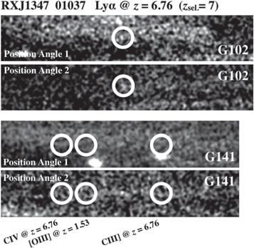
Figure 6. GLASS spectra of the confirmed Lyα emitter at z = 6.76, RXJ1347_01037, described in Section 7.1 and presented by Huang et al. (2015). The white circles in the G102 spectra mark the position of Lyα. The central white circles in the G141 spectra mark the position of [O iii] λ5007, if the line was [O ii] λ3727 at z = 1.35. The lack of [O iii] emission supports the interpretation that the G102 emission line is Lyα, given that a low-metallicity object at z = 1.35 would have [O iii]/[O ii] . The left- and rightmost white circles in the G141 spectra mark the location of C iv λ1549 and C iii] λ1909 at z = 6.76, respectively. We do not detect any significant C iv and C iii] emission from this object with line ratio limits of
  and
and ![${f}_{{\rm{C}}{\rm{III}}]}/{f}_{\mathrm{Ly}\alpha }\lesssim 0.25$](https://content.cld.iop.org/journals/0004-637X/818/1/38/revision1/apj521744ieqn112.gif) .
.
Download figure:
Standard image High-resolution imageIn the Keck-DEIMOS spectrum the blue side of the line falls on a sky line residual. Hence, even though the DEIMOS spectrum would resolve the [O ii] doublet at z = 1.53, the identification of the feature as Lyα at z = 6.76 from Keck is not fully conclusive (even though the asymmetric line profile is consistent with it). Unfortunately, in the GLASS spectra the resolution is too low to resolve the doublet.
However, GLASS can confirm the line identification as Lyα by virtue of its NIR spectral coverage. If the detected line were [O ii] λ3727, we would expect to see [O iii] λ5007 emission, based on typical line ratios. The DEIMOS wavelength coverage is not sufficient to look for potential [O iii] emission. GLASS, in contrast, has sufficient wavelength coverage in the G141 grism (these spectra are also shown in Figure 6). We do not detect any flux in the G141 spectra at  Å (marked by the central white circles in the G141 spectra in Figure 6), which would be the expected position of [O iii] λ5007 at z = 1.53. If the object is a low-metallicity object at z = 1.53, we expect [O iii]/[O ii]
  (e.g., Nagao et al. 2006; Maiolino et al. 2008), which is certainly not the case. A high-metallicity galaxy would show high ratios of [O ii]/[O iii], consistent with what is observed. However, as star-forming galaxies will always have either [O iii] or Hβ flux
  the [O ii] flux (Jones et al. 2015), the nondetection of Hβ makes such a scenario very unlikely. Combining the fluxes in the individual spectra (see below) and using the 2σ flux limits at the location of [O iii], the limit on the [O iii]/[O ii] ratio from the GLASS spectra becomes
 ![${f}_{2\sigma {\rm{lim.,}}[{\rm{O}}{\rm{III}}]}/{f}_{[{\rm{O}}{\rm{II}}]}\lesssim 0.32$](https://content.cld.iop.org/journals/0004-637X/818/1/38/revision1/apj521744ieqn116.gif) . Furthermore, the automatic line detection mentioned in Section 5 assigns a combined probability
. Furthermore, the automatic line detection mentioned in Section 5 assigns a combined probability  , which corresponds to a 4.01σ detection, of a line at 9440 ± 50 Å. Based on this probability, the nondetection of [O iii], and the [O iii]/[O ii] flux ratio limit, we conclude that the line detected in the GLASS and Keck-DEIMOS spectra is Lyα at z = 6.76, in agreement with the conclusion based on the line profile by Huang et al. (2015), and strongly favored by the photometry. Given the Lyα emission and the redshift, the GLASS wavelength coverage allows us to search for C iv λ1549 and C iii] λ1909 emission at 12020 and 14815 Å (marked by the left- and rightmost white circles in the G141 spectra in Figure 6). We do not detect any significant C iv or C iii] emission from RXJ1347_01037 in the GLASS spectra.
Estimating the Lyα line flux and equivalent width from the GLASS G102 spectra, we find (fluxes not corrected for magnification)


for the S/N = 2.6 line (PA 1 in Figure 6) and


for the S/N = 4.1 line (PA 2 in Figure 6), resulting in a combined line flux and equivalent width of


These two estimates are in mutual agreement, but in tension with the line flux and equivalent width estimated from the DEIMOS spectrum by Huang et al. (2015). They find a line flux of  and an Lyα equivalent width of
  Å. The GLASS and DEIMOS fluxes taken at face value differ by 4σ. We expect this difference to be caused by systematic uncertainties in the ground-based DEIMOS spectrum, including those stemming from a combination of slit losses, absolute spectrophotometric calibration, and sky line subtraction.
From the Lyα estimates we find the following upper limits on the rest-frame UV emission line ratios from RXJ1347_01037:


Here we have again used the 2σ flux limit on C iv and C iii].
7.2. MACS2129_00899
Another object worth highlighting is MACS2129_00899. It is a high-confidence Lyα emitter candidate at z = 8.10 that shows emission lines in both of the G102 spectra at 11065 Å. This wavelength is also covered by the G141 grisms, albeit at low sensitivity (see Figure 5). Despite the low sensitivity and relatively high contamination, there appears to be a marginal detection of the line in one of the G141 spectra as well. The estimated flux and equivalent widths of the G102 lines are quoted in Table 3 and are in mutual agreement with the combined line flux and Lyα equivalent width of


In the top panels of Figure 7 we show the G102 spectra, with the Lyα line marked by the white circles. Consistent with the photometric selection criteria listed in Table 3, the photometric redshift posterior distribution function (in the form of  ) shown in Figure 7 peaks at
  . The spectral energy distribution templates fitting the photometry best are also shown in Figure 7. This redshift estimate comes from an independent fit using a current version of zphot (Giallongo et al. 1998) based on independent HST and Spitzer photometry from SURFS-UP (Bradač et al. 2014) obtained following Huang et al. (2015). As is often the case for
  galaxy candidates, a local
  -minimum is also seen at redshift ∼2. In this case, the emission line could be [O ii] λ3727 at z = 1.97, and the observed break would be the 4000 Å break instead of the Lyα break. However, if the lower-redshift solution were correct, [O iii] λ5007 would fall at 14870 Å. As was the case for RXJ1347_01037, we do not detect any [O iii] emission in the GLASS G141 spectra, which supports the interpretation of the G102 emission feature as Lyα at z = 8.1. We do not detect any C iv at 14095 Å in the G141 spectra for this source either (C iii] will fall at 17371 Å, which is outside the G141 wavelength coverage). The limit on the C iv/Lyα flux ratio obtained from the GLASS spectra is
  , where we have again used the 2σ limiting flux for C iv. This limit is in good agreement with current estimates of C iv/Lyα flux ratios at intermediate and high redshift (Shapley et al. 2003; Erb et al. 2010; Stark et al. 2014, 2015a, 2015b), which are generally less than 0.6.
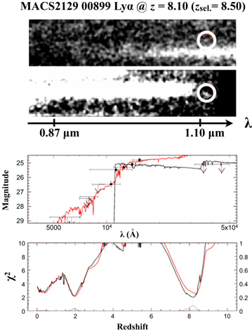
Figure 7. GLASS G102 spectra (top panels), photometry (central panel), and photometric redshift estimate  curve (bottom panel) for the candidate Lyα emitter at z = 8.1, MACS2129_00899. The photometry includes CH1 and CH2 IRAC 1σ upper limits from SURFS-UP (Bradač et al. 2014) obtained following Huang et al. (2015). The black
  curve in the bottom panel includes F160W, whereas the red curve does does not (F160W has potential contamination and therefore uncertain photometry). In both cases there are valid photometric redshifts around
  (black spectral energy distribution overplotted on the photometry in the center panel) and
  (red spectral energy distribution overplotted on the photometry in the center panel) with marginal statistical difference. The
  solution overestimates the 1σ IRAC constraints. If the line were [O ii] λ3727 at z = 1.97, we would expect to see [O iii] at roughly 14870 Å. We do not detect any [O iii] emission in the GLASS G141 spectra, consistent with the
  solution.
Download figure:
Standard image High-resolution imageIf confirmed, this would be one of the highest-redshift sources known to date, together with the recent z = 8.7 galaxy confirmed by Zitrin et al. (2015b) and the z = 8.2 γ-ray burst presented by Salvaterra et al. (2009) and Tanvir et al. (2009). However, owing to the relatively low resolution of the HST grisms and the low S/N of the lines presented here, deep high-resolution spectroscopic follow-up is needed to confirm the high-redshift nature of this source, or deeper photometry to further improve the photometric redshift estimate.
7.3. Two Potential Objects

As presented in Table 3, RXJ2248_00404 and MACS1423_01018 of the Silver_EL sample appear to have emission lines at 1.32 and 1.37 μm, respectively. If these lines are confirmed to be Lyα, this would place these objects at  . Figure 8 shows the G141 spectra, marking the detected emission lines with white circles. Both objects are selected as photometric dropouts, i.e., selected based on a few detections redward of the Lyman break and nondetections in bands blueward of the break. In both cases the EAzY photometric redshift distributions have highly probable solutions at
  –3, and the photometry is therefore inconclusive as to whether the objects are at high redshift or low redshift. If the emission lines are [O ii] at z = 2.55 and z = 2.68 for RXJ2248_00404 and MACS1423_01018, respectively, this would agree with the EAzY p(z) and rule out the color selections placing them at redshift 8 and 9. In case the sources are at redshift 2–3, the drop in the NIR colors used to select them as high-redshift galaxies could be attributed to the 4000 Å break as opposed to the Lyman break, which is known to be one of the main contaminants of Lyman break galaxy samples. The resolution of the G141 grism is too low to resolve the [O ii] doublet or detect the asymmetry of the Lyα line, and we therefore cannot distinguish between the two lines with the GLASS data. We also do not have the wavelength coverage to look for the [O iii] doublet, which would fall at 17775 and 18426 Å, respectively. In summary, the two potential
  objects might be contaminats showing [O ii] emission at
  , but without follow-up spectroscopy or deeper imaging we cannot rule out the high-redshift Lyα scenario.
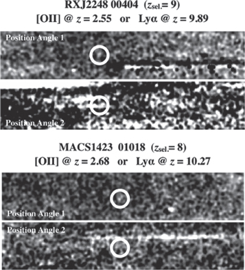
Figure 8. GLASS G141 spectra of the two potential line emitters at  from the Silver_EL sample. The white circles mark the detected line emission. The objects were selected as Lyman break dropouts. However, highly likely low-redshift solutions in the EAzY p(z) suggest that the lines could also be [O ii] at
  . Given the location of the lines at 1.32 and 1.37 μm, the G141 spectrum does not cover [O iii], and the resolution does not allow us to resolve the potential [O ii] doublet or detect the asymmetry of Lyα. With the current data we therefore cannot rule out the high-redshift scenario.
Download figure:
Standard image High-resolution image8. PHYSICAL PROPERTIES FROM Lyα EMITTERS
As described in the introduction, spectroscopically confirmed Lyα emitters at high redshift (and the nonconfirmations from follow-up campaigns) have proven very valuable for studying the early universe and the environment at the epoch of reionization (Pentericci et al. 2011, 2014; Caruana et al. 2012, 2014; Treu et al. 2012, 2013; Faisst et al. 2014; Tilvi et al. 2014). In particular, confirmed Lyα emitters fix the redshift of the object, resulting in improved prediction power from fitting stellar population synthesis models to the photometry. Assuming a set of stellar population models (e.g., Bruzual & Charlot 2003; Maraston 2005) to generate spectral energy distributions for galaxies at the emission-line redshift, and fitting them to the available photometry, can give estimates of physical quantities of the galaxies like total stellar mass (the normalization between the observed flux and best-fit model), the star formation rate, metallicity, and the age of the stellar populations, i.e., the galaxy (e.g., Labbé et al. 2006; Vanzella et al. 2011; Coe et al. 2013, 2014; Finkelstein et al. 2013; Huang et al. 2015; Oesch et al. 2015; Zitrin et al. 2015b). When performing the spectral energy distribution fitting, assuming a dust law can furthermore predict the dust content of the galaxy. This can be directly compared to the measured UV spectral slope, if available from the data (e.g., Bouwens et al. 2015; Finkelstein et al. 2015b; Oesch et al. 2015). Another direct comparison can be obtained from independently determining the star formation rate from scaling relations with the UV photometry (Kennicutt 1998; Madau et al. 1998). As part of our study of IRAC-detected high-redshift galaxies presented by Huang et al. (2015), we estimated the physical properties of the confirmed Lyα emitter presented in Section 7.1. An important aspect of this study was the availability of ancillary Spitzer photometry from SURFS-UP (Bradač et al. 2014). Photometry in the rest-frame optical falling in the Spitzer IRAC infrared bands for high-redshift galaxies has proven to be an important part of reliably predicting the physical properties of (high-redshift) galaxies through spectral energy distribution fitting (e.g., Schaerer & de Barros 2010; Labbé et al. 2013; Smit et al. 2014a, 2014b; Finkelstein et al. 2015a; Huang et al. 2015; Wilkins et al. 2015). Furthermore, fixing the redshift of the spectral energy distributions when fitting to photometry can also be used as a test of the validity of potential low-redshift contaminants. If, for instance, the best-fit low-redshift model predicts a dusty red and old stellar population, it would be very unlikely to see strong [O ii] emission, therefore making a high-redshift Lyα scenario more likely (Coe et al. 2013; Finkelstein et al. 2013). Similar arguments can be used to rule out other line-emitting low-redshift contaminants. Fixing the redshift of high-redshift sources behind massive clusters, like the ones presented in the current study behind the GLASS clusters, is not only important for the study of individual sources and high-redshift galaxy populations. Knowing the redshift, i.e., the luminosity distance to any object, precisely, especially if it is multiply lensed, is also very valuable for lens modeling of the foreground clusters (e.g., Coe et al. 2013, 2014; Zitrin et al. 2014). Lastly, the sizes of high-redshift galaxies have also been shown to provide useful information about the environment and epoch they inhabit (Ono et al. 2013; Curtis-Lake et al. 2014; Holwerda et al. 2015).
As exemplified by the objects described in Section 7, we expect several of the line emitters presented in Table 3 to be true Lyα emitters. However, as shown in Section 6, we also expect a considerable fraction of the objects to be contaminants resulting from either low-redshift line emitters or spurious line detections in the GLASS spectra. We therefore consider the current sample to be premature for a full spectral energy distribution study, including comparing their inferred physical properties given the expected low purity of the presented sample. An in-depth study of the purely photometric Gold and Silver samples is beyond the scope of this work, as it would benefit greatly from the inclusion of ancillary Spitzer photometry and a detailed knowledge of the purity and completeness functions of the complex heterogeneous photometric samples. We defer such a study to a future publication when the full HFF data are available and the SURFS-UP Spitzer data have been analyzed.
9. STACKING THE SPECTRA

The Lyα emission line has so far been the main rest-frame UV emission line used for spectroscopic confirmation of high-redshift (and to some extent low-redshift) galaxies owing to its characteristic spatial profile, strength, and accessibility in the optical/NIR. However, over the past several years, searches for and studies of other rest-frame UV lines like C iv λ1549 and C iii] λ1909 have shown that these are potentially strong enough to complement Lyα in the identification and studies of galaxies close to the epoch of reionization, where the optical depth to Lyα is expected to be high owing to the increasingly neutral IGM (e.g., Stark et al. 2010, 2011, 2013, 2014; Schenker et al. 2014). Observations of sources at redshifts below 3 (Shapley et al. 2003; Erb et al. 2010; Stark et al. 2014; Rigby et al. 2015) suggest that, indeed, C iii] (which is not affected by the neutral hydrogen in the IGM) might be strong enough for detection with current facilities. As a "proof of concept," two detections of C iii] (Stark et al. 2015a) and one of C iv (Stark et al. 2015b) in Lyα emitters at  have recently been presented. The C iii] emission is generally faint and therefore difficult to detect, and current estimates of
 ![${f}_{{\rm{C}}{\rm{III}}]}/{f}_{\mathrm{Ly}\alpha }$](https://content.cld.iop.org/journals/0004-637X/818/1/38/revision1/apj521744ieqn141.gif) at
at  from Stark et al. (2014) are
  . In fact, Zitrin et al. (2015a) searched for C iii] in a small sample of high-redshift galaxy candidates but were unable to confirm any C iii] emission. In Table 2 objects from this search overlapping with our samples have been marked by an asterisk.
Thus, even though it is challenging, a systematic search for the C iii] and C iv lines at redshifts close to the epoch of reionization would be extremely valuable to improve our understanding of the IGM and of the galaxies themselves. Detection of these UV lines would enable photoionization modeling of line strengths, improving our understanding of the stellar populations and metallicities of these galaxies (Stark et al. 2014) and ultimately of their output of ionizing photons.
As shown in Figure 5, the GLASS spectra reach limiting line fluxes of ∼5 × 10⁻¹⁸ erg s−1 cm−2. At this depth, we do not detect C iii] or C iv emission in the Gold_EL and Silver_EL samples. To improve the S/N, we stacked the GLASS spectra of the various samples to search for potential C iv and C iii] emission. Figure 9 shows the relevant parts of the rest-frame stacks (assuming the Lyα redshifts listed in Table 3) of the Gold_EL sample. The position of Lyα C iv and C iii] is marked by the white circles. We do not detect any continuum break redward of the Lyα emission in the stacks of the dropouts presented here. We do not detect any C iv and C iii] emission either. From the Gold_EL  stack we estimate the flux ratio limits between the rest-frame UV emission lines to be


where we used 2σ limiting fluxes for C iv and C iii] estimated on the stacked spectra. The  was also measured directly from the stack, as described in Section 4. These upper limits agree well with the
  ratios presented by Stark et al. (2015b) and the
 ![${f}_{{\rm{C}}{\rm{III}}]}/{f}_{\mathrm{Ly}\alpha }$](https://content.cld.iop.org/journals/0004-637X/818/1/38/revision1/apj521744ieqn147.gif) ratios for low-metallicity objects at intermediate and high z presented by Shapley et al. (2003), Erb et al. (2010), and Stark et al. (2014, 2015a), which range from 0.1 to 0.6 and 0.1 to 0.3, respectively.
ratios for low-metallicity objects at intermediate and high z presented by Shapley et al. (2003), Erb et al. (2010), and Stark et al. (2014, 2015a), which range from 0.1 to 0.6 and 0.1 to 0.3, respectively.
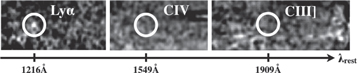
Figure 9. Cutouts of the stacked two-dimensional spectrum of the Gold_EL emission-line objects listed in Table 3. The mean redshift of the shown stack is  . The stacked Lyα, marked by the white circle on the left, appears compact and is not resolved (see top panel of Figure 10). There is no detection of a continuum break redward of the Lyα line. The stacks show no detection of C iv λ1549 and C iii] λ1909, as indicated by the two rightmost white circles.
Download figure:
Standard image High-resolution imageIn addition to allowing us to look for rest-frame UV lines, the stacked high-S/N spectra enable us to further test the hypothesis that the majority of the emission is Lyα at high redshift. Following a line of arguments similar to what was presented in Section 7, we would expect significant [O iii] emission in the GLASS spectra, should the majority of the sources be low-redshift [O ii] emitters, with the photometric dropout caused by the 4000 Å break. The stack does not show any flux excess at 5007 Å rest frame, and the line emission is therefore unlikely to come from low-redshift [O ii] emission.
Including the Silver_EL sample in the GLASS stack (or stacking the Silver_EL objects separately) does not change any of the above conclusions.
10. THE SPATIAL EXTENT OF Lyα AT

A unique feature of the GLASS spectra is the high angular resolution, owing to the sharp HST point-spread function (PSF) and the magnification by the foreground clusters. Thus, GLASS provides an opportunity to measure, for the first time, the angular extent of the Lyα emission. Spatial information is preserved in the extracted two-dimensional spectra, and the spatial extent of emission lines can in principle be estimated.
From the  Lyα stack presented in Section 9 we extracted the spatial profile of the Lyα emission, by collapsing a 20 Å window centered on the line in the dispersion direction (roughly the width of the circle marking the Lyα emission in Figure 9). The resulting profile is shown in green in the top left panel of Figure 10. In the same figure, the PSF of the data is shown in blue. The PSF was obtained by extracting the spatial profile from a stack of stellar spectra from the GLASS observations. We also extracted the spatial profile of the stacked NIR (rest-frame UV) images, representing the continuum light profile of the stack. This profile is shown in the top right panel of Figure 10. To determine whether the extent of Lyα and the rest-frame UV continuum deviates from the PSF, we modeled each of them as a Gaussian convolution of the PSF (G∗PSF) times a constant C. By sampling values of the standard deviation of the Gaussian convolution kernels (
 ) and estimating the minimum
  as
as
we can quantify the deviation of the spatial profiles from the PSF. In the expressions above,  and
and  refer to the ith pixel in the spatial profiles of the Lyα (or rest-frame UV) and the convolved PSF, respectively. The
  is the variance on the Lyα (or rest-frame UV) profile, and the constant C is minimized analytically by setting
  . The profiles of the convolved PSF minimizing
  are shown as the red curves in Figure 10 and correspond to Gaussian convolution kernels with
  pixels and
  pixels for the Lyα and rest-frame UV spatial profiles, respectively. Hence, both profiles are only marginally resolved, and there is no indication that the Lyα is more extended than the UV light in the stack.
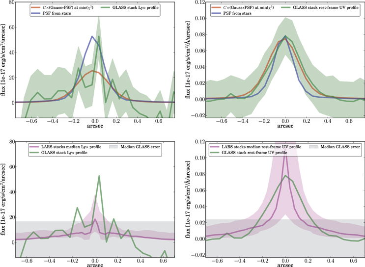
Figure 10. Spatial profiles of the stacked Gold_EL Lyα emitters at  (left, green curve) and their observed NIR (rest-frame UV) direct images (right, green curve). In the top panels these profiles are compared to the PSF represented by the spatial profile of stars (blue curves) in the GLASS fields of view. The red curves show the convolved PSF (multiplied by a constant C) that minimizes the
  between the PSF and the data. Both the Lyα and the rest-frame UV profiles from the GLASS stacks are unresolved. Hence, taken at face value, there is no evidence that the spatial extent of Lyα is more extended than the UV light in the GLASS stack. The bottom panels show a comparison to the median LARS Lyα and rest-frame UV profiles at z = 7.2 (see Section 10.1). The shaded area around the profiles shows the 1σ spread of the individual profiles. The median error on the GLASS stacks (from the top panel's green shaded region) is represented by the gray band. Based on this comparison, we conclude that the extended Lyα emission surface brightness typical of lower-redshift Lyman break galaxies is too faint to be detected in this GLASS stack.
Download figure:
Standard image High-resolution imageSeveral authors (e.g., Finkelstein et al. 2011; Steidel et al. 2011; Matsuda et al. 2012; Momose et al. 2014; Wisotzki et al. 2015) have shown that the Lyα emission is 5–15 times more extended than the continuum emission at redshifts  . Taking the results from GLASS at face value, the
  would seem to indicate more compact emission than at lower redshift. However, as described in the following section, the sensitivity of the GLASS stack is insufficient to detect the extended Lyα emission, and we are thus most likely only seeing the high surface brightness core.
10.1. Comparison to the LARS Sample
To quantify our ability to detect extended Lyα emission in our GLASS  stack, we carry out a systematic comparison with the rest-frame UV and Lyα emission in the LARS galaxies presented by Hayes et al. (2013, 2014) and Östlin et al. (2014).
The LARS sample consists of 14 low-redshift (all with  ) star-forming (SFR
 ; Hayes et al. 2014) Lyman break galaxy analogs. It has been observed extensively with HST from the UV to the optical (see Table 4 in Östlin et al. 2014). The wealth of data has enabled the creation of high-resolution rest-frame UV, Lyα, Hα, and Hβ maps, suitable for comparison with both low- and high-redshift counterparts. Following the prescription outlined by Guaita et al. (2015), we simulated the observations of 12 of the LARS galaxies redshifted to z = 7.2, the mean redshift of the GLASS stack (we also simulated z = 7 and z = 7.4 to verify the redshift sensitivity and found it to be negligible). We did not include LARS04 and LARS06, as they do not show any Lyα emission within the HST field of view.
In practice, the HST images of the LARS galaxies were resampled to a  pixel scale (similar to the
  used for the GLASS interlacing), corresponding to ∼0.2 kpc at z = 7.2, fixing the physical size and preserving flux as outlined by Guaita et al. (2015). After resampling, the Lyα and rest-frame UV emission was isolated via continuum subtraction using the "continuum throughput normalization" (CTN) factor as described by Hayes et al. (2005, 2009). The continuum-subtracted emission maps were then scaled based on luminosity distance and surface brightness dimming (e.g., Bouwens et al. 2004). For more details on the LARS sample and the high-redshift simulations, we refer the reader to Hayes et al. (2013, 2014), Östlin et al. (2014), and Guaita et al. (2015).
The individual spatial profiles of the LARS galaxies were produced by collapsing the UV and Lyα images after an arbitrary rotation around the rest-frame UV emission centroid. For each galaxy, these individual profiles were aligned and combined to a main spatial UV and Lyα profile for each of the 12 galaxies. This essentially corresponds to stacking 12 samples of N "different" galaxies. The medians of these 12 rest-frame UV and Lyα profiles are shown at a simulated redshift of 7.2 in magenta in the bottom panels of Figure 10. The shaded regions show the 68% spread of the 12 profiles. Comparing these profiles to the GLASS rest-frame UV and Lyα taking the median error on the GLASS stacks into account (horizontal gray band), it is clear that in most cases the extended Lyα emission would not be detectable in the GLASS stack. Only the central high surface brightness peak appears detectable with the GLASS sensitivity. In this simulation we have neglected the effect of magnification. If we scale up the LARS galaxies by the average linear magnification  , the effect is unchanged. If we only consider the LARS Lyα emitters (LAEs) (EW
 Å), the conclusions do not change either.
A similar conclusion is reached by comparing the surface brightness profiles and uncertainties of the GLASS stack with the Lyα surface brightness profiles presented by Momose et al. (2014) and Wisotzki et al. (2015), even though both of these studies are only considering redshifts lower than 7.
11. SUMMARY
In this paper we have presented a systematic search for Lyα emission from galaxies at the epoch of reionization. We have analyzed the GLASS spectroscopy of 159 photometrically preselected  galaxy candidates lensed by the first six clusters observed as part of GLASS. Our main results can be summarized as follows:
- 1.From visual inspection of all 159 spectra, we find emission features consistent with being Lyα in 24 objects. Assuming that the lines are all Lyα, the mean redshift of the emission-line sample is 7.3 (7.2 and 7.4 for the Gold_EL and Silver_EL sample, respectively), with a few candidates above. By comparison with automatic line detection results, we estimate the completeness of this sample to be 40%–100% with a purity of 60%–90%. Deeper spectroscopic follow-up is needed to improve the estimates of completeness and purity.
- 2.One of the candidates has been confirmed spectroscopically with DEIMOS on Keck. The long-wavelength coverage of the GLASS grism allows us to confirm that the line is indeed Lyα and not [O ii] at lower redshift.
- 3.The most compelling candidate at is detected independently in both of the G102 grism spectra (and marginally in one of the G141 spectra). The total line flux is erg s−1 cm−2, and the wavelength of the emission line corresponds to Lyα at z = 8.10, consistent with the photometric redshift. Follow-up spectroscopy or deeper imaging is needed to confirm the candidate.
- 4.The number of emission-line detections is consistent with the expectations based on our knowledge of the Lyα emission probability for Lyman break galaxies at, although the uncertainties are large. The full analysis of the GLASS sample, together with a homogenous selection based on the Hubble Frontier Field HST (and SURFS-UP Spitzer IRAC) imaging data set, is necessary to carry out a more quantitative analysis and measure the Lyα optical depth to and sources.
- 5.From a stack of the most promising Lyα emitters we derive the spatial profile of Lyα at. The stacked Lyα profile is comparable in size to that of the continuum UV emission and only marginally resolved with respect to the PSF. Diffuse Lyα, if present, is below our surface brightness detection limit. We show that this is consistent with the properties of galaxies at lower redshift, by simulating observations of the low-redshift LARS Lyman break galaxy analogs at z = 7.2.
- 6.We do not detect any C iv or C iii] emission in the stack, down to a 1σ Lyα limit of 2 × 10⁻¹⁸ erg s−1 cm−2 (not corrected for magnification).


In conclusion, our search has confirmed that Lyα is getting harder and harder to detect as we approach the epoch when the universe is in large part neutral. The space-based data guarantee that this is not due to the unfortunate coincidence of sky emission lines and redshifted Lyα. However, the extreme faintness of these lines requires even deeper follow-up spectroscopy, in order to make progress, by improving our estimates of completeness and purity. Higher spectral resolution data would also help remove contamination by detecting the characteristically asymmetric Lyα profile. We have published this first sample as quickly as possible with the aim of fostering follow-up efforts.
This paper is based on observations made with the NASA/ESA Hubble Space Telescope, obtained at STScI. Support for GLASS (HST-GO-13459) was provided by NASA through a grant from the Space Telescope Science Institute, which is operated by the Association of Universities for Research in Astronomy, Inc., under NASA contract NAS 5-26555. We are very grateful to the staff of the Space Telescope for their assistance in planning, scheduling, and executing the observations. B.V. acknowledges support from the World Premier International Research Center Initiative (WPI), MEXT, Japan, and the Kakenhi Grant-in-Aid for Young Scientists (B)(26870140) from the Japan Society for the Promotion of Science (JSPS). A.H. acknowledges support by NASA Headquarters under the NASA Earth and Space Science Fellowship Program—Grant ASTRO14F-0007. M.B., A.H., and K.H. also acknowledge support by NASA through an award issued by JPL/Caltech and from STScI via HST-AR-13235, HST-GO-13177, and special funding as part of the HST Frontier Fields program conducted by STScI. T.A.J. acknowledges support from the Southern California Center for Galaxy Evolution through a CGE Fellowship. This work utilizes gravitational lensing models produced by PIs Bradač Ebeling, Merten & Zitrin, Sharon, and Williams funded as part of the HST Frontier Fields program conducted by STScI. STScI is operated by the Association of Universities for Research in Astronomy, Inc., under NASA contract NAS 5-26555. The lens models were obtained from the Mikulski Archive for Space Telescopes (MAST).
APPENDIX A: GLASS CONFIRMATION OF z = 6.1 AND z = 6.4 LyαEMITTERS IN RXJ2248 AND MACS0717
Currently, two multiple-imaged systems at high redshift have been spectroscopically confirmed in the six clusters analyzed in this work. In RXC J2248.7–4431 Boone et al. (2013) and Balestra et al. (2013) presented spectroscopy of a multiple-imaged system at z = 6.1 and Vanzella et al. (2014b) confirmed a system in MACS0717 at z = 6.4. In Table 5 we list the individual components of these systems detected in the GLASS data. Owing to their  redshifts, these objects were not included in the sample of dropouts studied in this paper. As expected, the main components have photometric redshift estimates around 6, as shown by the 1σ intervals from EAzY quoted in Table 5.
Table 5. The Multiple-imaged Sources from Boone et al. (2013), Balestra et al. (2013), and Vanzella et al. (2014b)
| Cluster | ID | ID | R.A. | Decl. | F105W
|

|
P.A. |

|

|
EW
|

|
μ |
|---|---|---|---|---|---|---|---|---|---|---|---|---|
| GLASS | CLASH | (degree) | (degree) | (ABmag) |
 range range |
(degree) | (Å) | (Å) | (1e-17 erg s−1 cm−2) | |||
| RXJ2248 | 00699 | 01291 | 342.19089 | −44.53746 | 24.82 ± 0.04 | [5.807,5.940] | 053, 133 | 8641, 8613 | 6.106, 6.083 | 45 ± 8, 46 ± 8 | 5.54 ± 1.01, 5.59 ± 0.94 | 4.26 ± 2.85 |
| RXJ2248 | 00845 | 01154 | 342.18104 | −44.53463 | 25.09 ± 0.06 | [0.065,0.183] | 053, 133 | 8638, 8642 | 6.104, 6.107 | 53 ± 11, 63 ± 14 | 5.03 ± 1.01, 5.99 ± 1.29 | 3.74 ± 5.32 |
| RXJ2248 | 01131 | 00847 | 342.18904 | −44.53002 | 24.29 ± 0.03 | [0.912,1.053] | 053, 133 | 8635, 8640 | 6.101, 6.105 |
 a,
a,  a
a
|
 a,
a,  a
a
|
4.16 ± 8.35 |
| RXJ2248 | 01752 | 00401 | 342.17130 | −44.51981 | 25.94 ± 0.08 | [5.789,5.994] | 053, 133 | 8650, 8633 | 6.113, 6.100 | 77 ± 24, 46 ± 20 | 3.35 ± 1.02, 1.99 ± 0.88 | 2.03 ± 1.2 |
| MACS0717 | 00846 | 01730 | 109.40773 | 37.74274 | 26.42 ± 0.11 | [5.745,5.989] | 020, 280 | 8985, 8985 | 6.389, 6.389 |
 a,
a,  a
a
|
 a,
a, a
a
|
10.96 ± 13.39 |
| MACS0717 | 02068 | 00859 | 109.40907 | 37.75469 | 26.34 ± 0.16 | [5.846,6.084] | 020, 280 | 8980, 8987 | 6.385, 6.391 | 78 ± 33, 134 ± 45 | 2.11 ± 0.86, 3.62 ± 1.16 | 8.15 ± 6.63 |
Note.
aFlux and EW estimates are tentative owing to high contamination in the GLASS spectra. μ gives the magnifications of the HFF clusters obtained as described in Section 4.Download table as: ASCIITypeset image
We list the apparent position of the Lyα emission line in the GLASS G102 spectra and the corresponding redshift. In a few cases, significant flux contamination at the location of Lyα makes the flux estimates, and hence the equivalent widths, only tentative. In Figure 11 we compare the equivalent widths from GLASS with the values quoted in the literature.

Figure 11. Equivalent widths estimated from the detections of Lyα in the individual GLASS spectra of the four main images of the multiple-imaged system at z = 6.1 from Boone et al. (2013) and Balestra et al. (2013) (left part) and the two images of the z = 6.4 Lyα emitter from Vanzella et al. (2014b) (right part) listed in Table 5. The equivalent widths estimated by Balestra et al. (2013) and Vanzella et al. (2014b) are marked by the dotted and dashed lines, respectively. The shaded regions indicate the quoted uncertainties. The gray dots represent GLASS spectra, with severe contamination at the location of Lyα making the GLASS equivalent width estimates only tentative. The arrow indicates that the tentative estimate of MACS0717_00846 at PA = 020 is outside the plotted range. The equivalent width estimates from the GLASS spectra generally agree with each other. There is marginal agreement with the Vanzella et al. (2014b) estimates, whereas the GLASS equivalent widths are generally lower than the estimate from Balestra et al. (2013).
Download figure:
Standard image High-resolution image
Combining the equivalent width for the pairs of GLASS spectra, we find EW Å, EW
Å, EW Å, and EW
 Å for RXJ2248_00699, RXJ2248_00845, and RXJ2248_01752, respectively. These all agree within 1σ of each other. However, when comparing RXJ2248 GLASS equivalent widths with the equivalent width published by Balestra et al. (2013), we find a discrepancy of 5.7σ. If we combine the six (3 sources × 2 PAs) GLASS equivalent widths, we get EW
 , and this discrepancy shrinks to 4.8σ. For MACS0717 we find a combined Lyα equivalent width of EW
 Å, which is within 2.4σ of the 45 Å estimated for this source by Vanzella et al. (2014b).
In summary, the individual GLASS estimates are self-consistent but seem to disagree somewhat with the ground-based measurements for the RXJ2248 system. This discrepancy might also be explained by a combination of slit losses and the challenging modeling of the contamination and background subtraction in the GLASS spectra.
APPENDIX B: THE AUTOMATIC LINE DETECTION SIGNIFICANCE FOR THE EMISSION-LINE SAMPLES
In Table 6 we quote the line detection significance from the Bayesian line detection algorithm described in Section 5 and M.V. Maseda et al. (2016, in preparation) applied to the emission-line sample from Table 3. The quoted values correspond to the maximum p-values in the ± 50 Å range around the visually detected emission lines given in the " Å" column of Table 6 (and Table 3).
Table 6. Automatic Line Detection Significance of the Emission-line Samples from Table 3
| Cluster | ID | R.A. | Decl. | P.A. |

|

|
σ |
 a
a
|
|---|---|---|---|---|---|---|---|---|
| GLASS | (degree) | (degree) | (degree) | ( ± 50 Å) | ||||
| A2744 | 00463 | 3.604573038 | −30.409357092 | 135, 233 | 9395, ... | 0.9976003, 0.8201783 | 3.04, 1.34 | 3.32 |
| A2744 | 00844 | 3.570068923 | −30.403715689 | 135, 233 | 8929, ... | 0.9709888, 0.8801960 | 2.18, 1.56 | 2.68 |
| MACS1423 | 00648 | 215.945534620 | 24.072435174 | 008, 088 | 9585, ... | 0.9899920, 0.5552243 | 2.58, 0.76 | 2.69 |
| MACS1423 | 01102 | 215.935869430 | 24.078415134 | 008, 088 | 9681, ... | 0.8870970, 0.9054205 | 1.59, 1.67 | 2.31 |
| MACS2129 | 00677 | 322.353239440 | −7.697441500 | 050, 328 | 9582, 9582 | 0.9995228, 0.9999788 | 3.49, 4.25 | 5.50 |
| MACS2129 | 00899 | 322.343220360 | −7.693382243 | 050, 328 | 11059, 11069 | 0.5700795, ... | 0.79,... | 0.79 |
| MACS2129 | 01516 | 322.353942530 | −7.681646419 | 050, 328 | 9593, ... | 0.9810597, 0.9870194 | 2.35, 2.48 | 3.42 |
| RXJ2248 | 00207 | 342.185601570 | −44.547224418 | 053, 133 | 11609,... | 0.9801501, ... | 2.33,... | 2.33 |
| A2744 | 00233 | 3.572513845 | −30.413266331 | 135, 233 | 11156,... | 0.7343585, ... | 1.11,... | 1.11 |
| A2744 | 01610 | 3.591507273 | −30.392303082 | 135, 233 | ..., 8406 | 0.9998119, 0.9999839 | 3.73, 4.31 | 5.70 |
| A2744 | 02273 | 3.586488763 | −30.381334667 | 135, 233 | 8717, ... | 0.9890780, 0.9889105 | 2.55, 2.54 | 3.60 |
| MACS0717 | 00370 | 109.377007840 | 37.736462661 | 020, 280 | 9138, ... | 0.9377069, ... | 1.86,... | 1.86 |
| MACS1423 | 00435 | 215.942403590 | 24.069659639 | 008, 088 | 10500,... | 0, 
|
0, 0 | 0 |
| MACS1423 | 00539 | 215.932958480 | 24.070875663 | 008, 088 | 8666, ... | 0.7680499, 0.9973003 | 1.20, 3.00 | 3.23 |
| MACS1423 | 01018 | 215.958132710 | 24.077013896 | 008, 088 | 13702,... | 0.9201682, 0.2224523 | 1.75, 0.28 | 1.77 |
| MACS1423 | 01169 | 215.942112130 | 24.079404012 | 008, 088 | 9721, ... | 0.9998913, 0.8989955 | 3.87, 1.64 | 4.20 |
| MACS1423 | 01412 | 215.947908420 | 24.082450925 | 008, 088 | 9448, ... | 0.7569422, 0.9116211 | 1.17, 1.70 | 2.06 |
| MACS1423 | 01619 | 215.935606220 | 24.086476168 | 008, 088 | 9932, ... | 0.9972566, 0.9264660 | 3.00, 1.79 | 3.49 |
| MACS2129 | 01182 | 322.344533970 | −7.688477035 | 050, 328 | 12145,... | 0.9363897, 0.6058985 | 1.85, 0.85 | 2.04 |
| RXJ1347 | 00627 | 206.893075800 | −11.760237310 | 203, 283 | 10750,... | 0.9998887, 0.9416673 | 3.86, 1.89 | 4.30 |
| RXJ1347 | 00997 | 206.895685760 | −11.754637616 | 203, 283 | 9467, 9463 | 0.8859983, 0.9065139 | 1.58, 1.68 | 2.31 |
| RXJ1347 | 01241 | 206.899894840 | −11.751082858 | 203, 283 | 9902, ... | 0.8757706, 0.9886466 | 1.54, 2.53 | 2.96 |
| RXJ2248 | 00404 | 342.201879400 | −44.542663866 | 053, 133 | 13239,... | 0.0000187, 0.5989891 | 0, 0.84 | 0.84 |
| RXJ2248 | 01953 | 342.192399500 | −44.515663484 | 053, 133 | ..., 9118 | 0.9997395, 0.9626378 | 3.65, 2.08 | 4.20 |
Notes. The individual  values represent the maximum p-value in the range
  Å.
Å.
 is the individual significance estimates (σ) summed in quadrature.
Download table as: ASCIITypeset image
APPENDIX C: ESTIMATING PURITY AND COMPLETENESS
In this appendix we describe in detail the procedure adopted to estimate the purity and completeness of the visual and automated line detection. Here the completeness is defined as the number of detected lines divided by the number of lines from the selected galaxies above some flux limit. The purity is the number of actual lines divided by the number of detected lines. Hence, the completeness here only refers to our ability to detect emission lines among the selected galaxies and is therefore independent of the purity and completeness of the photometric preselections described in Section 3.1.
Let us write the notation for a single sample, using numerical examples from the Gold sample, when necessary, and for 3σ detections. Assuming that there are Nw lines above the flux limit that are well described in their morphology by the UV continuum and Nn that are not, the number of detections by the automated procedure will be

where ca is the completeness of the automated procedure,  is the rate of spurious detections per spectrum, and NG is the total number of spectra to be analyzed. The equivalent for the visual inspection procedure will be

For the Gold sample the numerical values are NG = 48 and  . Analysis of the output of the automated detection software yields
  above 3σ, after removing obviously spurious features at low grism sensitivity regions and from contamination subtraction residual. Roughly 60% of these lines were not picked up by the visual classification described in Section 3.3. One of these lines is the confirmed Lyα emitter RXJ1347_01037 (see Section 7).
We know from our analysis of the spectra in empty parts of the sky that  . Considering 3σ detections, we can assume that ca = 1 for all practical purposes. Thus,

Since Nw is positive, we conclude that it is in the range 0–8. In order to estimate the other quantities, we make use of the fact that approximately 40% of the lines detected automatically are also detected visually. Thus,

which can be written as

To solve this, we can assume conservatively that the human eye rejects with equal probability true and false positives, so that cv = 0.4 and  . Alternatively, we could optimistically assume that the human eye is better at removing false positives, and therefore
  is as small as possible (0.02) and cv = 1. This gives us a range of solutions for cv and fs, with the visual completeness being between 40% and 100%. The number of lines in the sample not well described by the UV flux that could potentially be detected is thus
ranging from 9 to 3 for the values of completeness estimated above. We can use the numbers derived here to assess the total purity of the sample, i.e., the fraction of true positives among the visual detections as

which ranges between 60% and 90% for the assumptions about completeness given above.
Repeating the arguments for the Silver sample with  , NG = 87 gives purity in the range 65%–90% for the same assumptions about completeness.
Footnotes
- 12
- 13
Here, contaminants refer to both faint low-z line emitters resembling Lyα emitters at high redshift, as well as features in the spectra not necessarily stemming from true astronomical sources. We note that all obvious defects and zeroth-order images were removed from the contaminants before purity and completeness were estimated. The fraction of faint low-z line emitters is confirmed to be small from a stack of the emission-line sources, as described in Section 9.