


ABSTRACT
NP Per is a well-detached, 2.2 day eclipsing binary whose components are both pre-main-sequence stars that are still contracting toward the main-sequence phase of evolution. We report extensive photometric and spectroscopic observations with which we have determined their properties accurately. Their surface temperatures are quite different: 6420 ± 90 K for the larger F5 primary star and 4540 ± 160 K for the smaller K5e star. Their masses and radii are 1.3207 ± 0.0087 solar masses and 1.372 ± 0.013 solar radii for the primary, and 1.0456 ± 0.0046 solar masses and 1.229 ± 0.013 solar radii for the secondary. The orbital period is variable over long periods of time. A comparison of the observations with current stellar evolution models from MESA indicates that the stars cannot be fit at a single age: the secondary appears significantly younger than the primary. If the stars are assumed to be coeval and to have the age of the primary (17 Myr), then the secondary is larger and cooler than predicted by current models. The Hα spectral line of the secondary component is completely filled by, presumably, chromospheric emission due to a magnetic activity cycle.
Export citation and abstract BibTeX RIS
1. INTRODUCTION
NP Per (classified EA/DM, mag. 11.53-12.35, TYC 2371-0390-1, spectral type :G4) was found to be an eclipsing binary star by Perova et al. (1966) from photographic plates. They proposed an orbital period of about 2.229 days, which is close to the currently adopted period. Later, Kholopov (1975) suggested a period twice this value, which we now know is not the case. The error was due to the very shallow secondary eclipses. Little else has been published on this star until now, except for some times of minimum light. NP Per is projected against the region of the Perseus star-forming complex (Belikov et al. 2002a), which suggests that it may be a very young object worthy of investigation. Few such pre-main-sequence (PMS) systems have been studied in detail (see, e.g., Stassun et al. 2014). Here, we report our extensive photometric observations using two robotic telescopes, as well as spectroscopic observations which, when combined, allow us to determine accurate absolute properties for the components. The spectroscopic orbital results are discussed in Section 2, the disentangling of the spectra in Section 3, and the photometric orbital solution in Section 4. We report the absolute dimensions in Section 5, followed by a comparison with theory in Section 6. We conclude with a discussion and final remarks.
2. SPECTROSCOPIC OBSERVATIONS AND ORBITS
From 2011 November through 2014 November, we acquired 56 high-quality spectra of NP Per with the Tennessee State University 2 m Automatic Spectroscopic Telescope (AST) and a fiber-fed echelle spectrograph (Eaton & Williamson 2007) at Fairborn Observatory in southeast Arizona. Of these spectra, 55 were suitable for radial velocity measurements. All of the spectra had 60 minute exposures. The detector for these observations was a Fairchild 486 CCD, having 4096 × 4096 15 micron pixels. While the spectrograms have 48 orders ranging from 3800 to 8260 Å, we have used just the orders that cover the wavelength region from 4920 to 7100 Å. Because of the faintness and moderately rapid rotation of NP Per, we made our observations with a fiber that produced a spectral resolution of 0.4 Å, corresponding to a resolving power of 15,000 at 6000 Å. Our spectra have typical signal-to-noise ratios (S/Ns) of 40 at 6000 Å. See Fekel et al. (2013) for additional information about the AST facility.
Fekel et al. (2009) gave a general explanation of the velocity measurement of our Fairborn echelle spectra. Briefly, using the lines in our solar-type star list, we measured radial velocities of both components. Those velocities were determined by fitting the individual lines with rotational broadening functions (Lacy & Fekel 2011), and we allowed both the depth and width of the line fits to vary. Our unpublished measurements of several IAU solar-type velocity standards show that these Fairborn Observatory velocities have a zero-point offset of −0.6 km s−1 when compared to the results of Scarfe (2010). So, we have added 0.6 km s−1 to each velocity. Our spectroscopic observations and those velocities are given in Table 1. Our rotational broadening fits of lines in our spectra with the highest S/Ns, result in v sin i values of 31 ± 2 km s−1 and 29 ± 3 km s−1 for components A and B, respectively. Adopting the photometric period, we initially computed an eccentric orbital solution for the primary. However, that solution produced a very small eccentricity of 0.0028 ± 0.0015. Because of that result and the circular orbit conclusion from the photometric solution, we next determined separate circular orbits of the two components. A comparison of the two solutions shows that the two center-of-mass velocities differ by just 0.6 km s−1, a 2σ result.
Table 1. Heliocentric Radial Velocities for NP Per
| HJD-2400000 | Phase | RVA (km s−1) | (O–C)A (km s−1) | RVB (km s−1) | (O–C)B (km s−1) |
|---|---|---|---|---|---|
| 55888.6338 | 0.906 | 96.0 | −1.3 | −86.0 | −3.1 |
| 55931.8785 | 0.311 | −19.5 | −1.3 | 65.1 | 2.2 |
| 55944.7593 | 0.091 | 97.0 | −1.1 | −87.7 | −3.7 |
| 55955.7729 | 0.033 | 111.9 | 0.6 | −100.8 | −0.2 |
| 55966.8044 | 0.983 | 113.5 | 0.7 | −105.9 | −3.4 |
| 55977.6716 | 0.859 | 78.9 | 0.6 | −59.9 | −0.9 |
| 55983.6697 | 0.551 | −72.1 | 1.1 | 132.0 | −0.4 |
| 56193.8200 | 0.849 | 73.0 | −0.4 | −55.4 | −2.7 |
| 56199.8150 | 0.539 | −75.4 | −0.2 | 132.6 | −2.3 |
| 56200.7967 | 0.980 | 111.8 | −0.7 | −99.4 | 2.8 |
| 56202.8352 | 0.894 | 93.3 | 0.4 | −77.6 | −0.1 |
| 56203.8088 | 0.331 | −30.0 | −1.0 | 78.0 | 1.4 |
| 56207.8337 | 0.137 | 80.0 | 0.1 | −62.0 | −1.0 |
| 56209.8305 | 0.033 | 110.6 | −0.6 | −98.4 | 2.2 |
| 56211.8211 | 0.926 | 103.6 | 0.4 | −89.7 | 0.8 |
| 56213.8194 | 0.823 | 60.4 | 0.4 | −34.3 | 1.6 |
| 56215.7696 | 0.698 | −13.3 | −0.3 | 54.1 | −2.2 |
| 56216.7977 | 0.159 | 69.5 | 0.3 | −50.8 | −3.3 |
| 56221.7592 | 0.386 | −54.4 | 0.0 | 108.5 | −0.2 |
| 56223.8068 | 0.305 | −15.3 | −0.8 | 57.7 | −0.5 |
| 56225.7405 | 0.172 | 62.2 | −0.3 | −42.0 | −2.9 |
| 56226.7933 | 0.645 | −41.5 | −0.3 | 90.4 | −1.5 |
| 56229.7452 | 0.969 | 111.3 | −0.2 | −98.8 | 2.1 |
| 56231.7664 | 0.876 | 86.8 | 1.0 | −67.4 | 1.0 |
| 56235.7683 | 0.672 | −26.4 | 1.1 | 72.0 | −2.6 |
| 56236.7704 | 0.122 | 86.8 | 0.1 | −72.0 | −2.4 |
| 56237.7540 | 0.563 | −70.0 | 0.7 | 126.1 | −3.1 |
| 56238.6998 | 0.987 | 113.0 | 0.0 | −101.5 | 1.3 |
| 56243.0070 | 0.920 | 101.1 | −0.4 | −89.6 | −1.3 |
| 56245.7296 | 0.142 | 78.1 | 0.3 | −60.4 | −2.0 |
| 56250.6718 | 0.359 | −43.6 | −0.6 | 93.1 | −1.2 |
| 56254.6537 | 0.146 | 76.1 | 0.3 | −57.7 | −1.9 |
| 56255.8592 | 0.687 | −18.4 | 0.8 | 64.6 | 0.4 |
| 56256.6542 | 0.044 | 109.7 | 0.0 | −99.3 | −0.6 |
| 56257.6970 | 0.512 | −77.4 | 0.4 | 134.2 | −3.9 |
| 56265.7523 | 0.126 | 85.3 | 0.5 | −70.9 | −3.8 |
| 56266.8344 | 0.612 | −55.8 | −0.4 | 110.9 | 1.0 |
| 56267.8187 | 0.053 | 107.4 | −0.6 | −97.0 | −0.6 |
| 56271.7299 | 0.808 | 51.2 | −0.8 | −24.5 | 1.3 |
| 56272.8091 | 0.293 | −7.5 | 0.3 | 53.2 | 3.5 |
| 56274.8209 | 0.195 | 50.0 | 0.2 | −22.4 | 0.5 |
| 56279.8718 | 0.462 | −74.1 | 1.2 | 132.8 | −2.2 |
| 56289.8557 | 0.942 | 108.9 | 1.9 | −97.1 | −1.9 |
| 56305.8223 | 0.106 | 93.4 | 0.7 | −78.6 | −1.4 |
| 56309.8212 | 0.901 | 94.9 | −0.4 | −79.1 | 1.3 |
| 56310.7919 | 0.336 | −32.5 | −0.8 | 77.8 | −2.2 |
| 56311.8441 | 0.808 | 52.3 | 0.3 | −25.4 | 0.3 |
| 56339.6960 | 0.306 | −15.2 | 0.2 | 60.5 | 1.2 |
| 56554.8542 | 0.851 | 74.7 | 0.2 | −51.6 | 2.6 |
| 56573.8124 | 0.358 | −42.5 | 0.0 | 93.9 | 0.3 |
| 56629.7521 | 0.459 | −73.8 | 1.1 | 131.5 | −3.1 |
| 56656.9124 | 0.647 | −41.6 | −1.4 | 93.5 | 2.8 |
| 56669.8128 | 0.435 | −69.1 | 1.1 | 130.4 | 1.8 |
| 56686.8103 | 0.062 | 107.5 | 1.5 | −92.7 | 1.3 |
| 56977.7936 | 0.632 | −47.2 | −0.1 | 100.0 | 0.7 |
(A machine-readable version of the table is available.)
From the variances of the two solutions the velocities of the primary and secondary were assigned weights of 1.0 and 0.15, respectively. We then combined the weighted velocities into a two component solution. Table 2 lists the resulting elements for this circular solution and related parameters. A circular solution of the combined data with the period as a free parameter resulted in P = 2.2285889 ± 0.0000063 days, which differs by 2.5 sigma from a more precise photometric value of 2.22857242 ± 0.00000012 days. Our Fairborn radial velocities are compared with the calculated velocity curves of the primary and secondary in Figure 1, where zero phase is a time of maximum velocity.
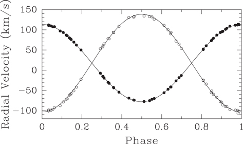
Figure 1. Radial velocities of the components of NP Per compared with the computed orbit. Filled circles = star A, open circles = star B. Zero phase is a time of maximum velocity of the more massive star A. It occurs 0.25 phase units before the deeper mid-eclipse in the light curve.
Download figure:
Standard image High-resolution imageTable 2. NP Per Spectroscopic Orbital Elements
| Parameter | Star A | Star B |
|---|---|---|
| P (days) | 2.22857242 (adopted) | |
| To (HJD) | 2456432.6139 ± 0.0005 | |
| e | 0.0 (adopted) | |
| w (deg) | 0.0 (adopted) | 180.0 (adopted) |
| K (km s−1) | 95.67 ± 0.14 | 120.85 ± 0.37 |
| g (km s−1) | 17.64 ± 0.10 | |
| m sin3i (solar masses) | 1.3083 ± 0.0086 | 1.0357 ± 0.0046 |
| a sini (106 km) | 2.9318 ± 0.0044 | 3.7035 ± 0.0113 |
| q = MB/MA | 0.7916 ± 0.0043 | |
| s(km s−1) | 0.8 | 2.1 |
| Observations | 55 | 55 |
Note.
*To is a time of maximum velocity for the more massive star, Star A.
Download table as: ASCIITypeset image
3. ATMOSPHERIC PARAMETERS AND METALLICITY FROM SPECTRAL DISENTANGLING
The spectra of double-lined binary stars are often rather complicated to analyze due to severe and variable line blending caused by Doppler shifts in the course of orbital motion, which is only exacerbated if the stars are rapidly rotating. A reliable determination of the atmospheric parameters and chemical composition of the components is greatly simplified by disentangling the spectra. The method of spectral disentangling (hereafter SPD) was developed by Simon & Sturm (1994) as a generalization of a tomographic separation technique introduced earlier by Bagnuolo & Gies (1991). In SPD, the individual spectra of the components as well as a set of orbital elements can be optimized simultaneously. This obviates the need to derive radial velocities, which are required as an input for the tomographic procedure of Bagnuolo & Gies (1991).
For the present work we have used the disentangling code FDBinary (Ilijic et al. 2004), which operates in Fourier space based on the prescription of Hadrava (1995). As the orbital elements for NP Per are well known (Section 2), we applied SPD in pure separation mode to obtain the component spectra. Restricting the analysis to observations out of eclipse, such as we have for NP Per, the disentangled spectra remain in the common continuum level of the total light of the binary, which is preserved in the process. Renormalization is therefore required for a proper atmospheric analysis of the individual spectra. External information is needed for this, typically in the form of the flux ratio between the components (eg., Hensberge et al. 2000, Pavlovski & Hensberge 2005).
We used 56 spectra of NP Per for SPD, including one that was of insufficient quality for use in determining its radial velocity. No weights were assigned to the observed spectra in SPD. One spectrum with a low S/N did not influence the SPD and the quality of the disentangled spectra, which we did check carefully. Corrections for the blaze function, continuum normalization, and merging of the echelle orders was performed following the procedures recommended by Kolbas et al. (2015). Proper continuum normalization is a critical step to avoid undulations in the disentangled spectra, as is having sufficiently complete phase coverage, which in our case we have. We selected two spectral regions for disentangling, based on the spectral information content and the desire to avoid contamination from telluric lines: one spans the range 5000–5800 Å, and the other the range 6540–6800 Å and includes Hα and the Li 6707 Å line. These spectral windows were further split into shorter segments of 50–100 Å, depending on the availability of line-free continuum windows. Special care was taken to select the edges of each segment at the continuum level, as errors in this process can negatively impact Fourier SPD affecting the line strength for lines close to the edges (e.g., Hensberge et al. 2008). Therefore, segments selected for SPD were always chosen in such a way that edges of contiguous segments overlapped by at the least one quarter of their lengths, so that the strength of the lines at the segment edges could be checked for consistency. Sections of the disentangled spectra for the primary and secondary are shown in Figure 2 on the continuum scale of the combined light.
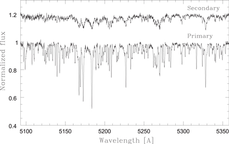
Figure 2. Portion of the disentangled spectra of the primary (bottom) and secondary (top) compononts of NP Per. The secondary's disentangled spectrum is shifted by +0.2 for clarity. The plots represent the separated components' spectra, i.e., these spectra are still in the common continuum of the binary's total light. These spectra are available in the on-line edition of the Journal as Tables 4 and 5.
Download figure:
Standard image High-resolution imageFor the renormalization of the disentangled spectra needed to recover the individual continua (see Hensberge et al. 2000, Pavlovski & Hensberge 2005) we adopted a prescription for the flux ratio between the components that is a function of wavelength. As described in more detail in Section 5, a first approximation to the flux ratio was obtained from initial estimates of the effective temperatures based on color indices and information from the light curve analysis, along with synthetic spectra computed with PHOENIX model atmospheres from Husser et al. (2013). Preliminary temperatures for both stars obtained as described below were then measured from the component spectra renormalized in this way, and the process was repeated, resulting in only minor changes to the flux ratio and temperatures. The secondary of NP Per is roughly 10 times fainter than the primary at 5000 Å, and 5 times fainter at Hα.
As the method of SPD effectively co-adds the flux from the observed spectra in constructing the disentangled spectra, the latter gain in S/N compared to our observations and this makes it possible to perform a detailed atmospheric analysis. The S/Ns from SPD are approximately 265 for the primary and 40 for the secondary in the visible region of the spectrum. These S/Ns were measurements in the disentangled spectra as a mean in five short windows in the continua. The most numerous lines in the primary are from Fe i. We used the UCLSYN code (Smalley et al. 2001) to measure equivalent widths for a selection of these lines taken from the compilation by Bruntt et al. (2012). The effective temperature of the primary along with its micro-turbulent velocity were determined in the standard way from the Fe i lines using the condition of excitation balance, and imposing a null correlation between the iron abundance and the reduced equivalent widths, respectively. The surface gravity was held fixed at log g = 4.28, close to the value adopted in the next section. Abundances were calculated in LTE using Kurucz (1979) model atmospheres, with reference to the standard scale of Asplund et al. (2009). We were able to derive abundances for four species in the primary star: Fe i, Ni i, Cr i, and Ti i. These results, along with the measured effective temperature and microturbulent velocity, are listed in Table 3. The uncertainties we report include contributions from the temperature and microturbulence errors, as well as the intrinsic scatter from the lines. The dominant contribution to the uncertainties in the abundances for all species examined is the uncertainty in the determination of the effective temperature. That these uncertainties are very similar could be either a coincidence, or the result of our careful selection of lines with good atomic data, resulting in a similar scatter. The renormalized disentangled spectrum of the secondary has too small a S/N to allow accurate abundance determinations, though we were able to derive its effective temperature from an optimal fit (Tamajo et al. 2011) to the renormalized spectrum over the 5050–5700 Å region, albeit with much larger uncertainty than the primary. A search for the signatures of a third star in the system's spectra by using SPD was negative. FDBinary was used in the mode for disentangling triple systems in a hierarchical triple system with a tentative third component in the outer orbit. This procedure was applied to several spectral windows. We obtained as well estimates of the projected rotational velocities for both stars, which we also list in Table 3. The separate disentangled spectra of the components are included with the on-line version of this article (Tables 4 and 5).
Table 3. Results of the Spectroscopic Analysis
| Quantity | Primary | Secondary |
|---|---|---|
| Teff (K) | 6420 ± 90 | 4540 ± 160 |
| log g (cgs) | 4.28 | 4.28 |
| vturb (km s−1) | 1.2 ± 0.1 | ⋯ |
| v sin i (km s−1) | 33.5 ± 0.9 | 33.3 ± 1.4 |
| Abundance for the Primary | ||
| [X/H] | N lines | |
| [Ti/H] | +0.07 ± 0.11 | 12 |
| [Cr/H] | −0.02 ± 0.08 | 32 |
| [Fe/H] | +0.02 ± 0.08 | 111 |
| [Ni/H] | −0.01 ± 0.10 | 41 |
Download table as: ASCIITypeset image
Table 4. Disentangled Spectrum of the Primary Component of NP Per
| Wavelength (Å) | Flux |
|---|---|
| 5033.782 | 0.97658 |
| 5033.854 | 0.97773 |
| 5033.926 | 0.97182 |
| 5033.998 | 0.99244 |
(Only a portion of this table is shown here to demonstrate its form and content. A machine-readable version of the full table is available.)
Download table as: DataTypeset image
Table 5. Disentangled Spectrum of the Secondary of NP Per
| Wavelength (Å) | Flux |
|---|---|
| 5033.782 | 0.97832 |
| 5033.854 | 0.99357 |
| 5033.926 | 0.99244 |
| 5033.998 | 0.98862 |
| 5034.070 | 0.97915 |
(Only a portion of this table is shown here to demonstrate its form and content. A machine-readable version of the full table is available.)
Download table as: DataTypeset image
The abundances derived for the primary star, which we assume also represent those of the secondary, are all close to solar within 1 sigma. Given the presumed youth of these stars (Belikov et al. 2002a), we made an effort to measure the lithium abundance in both components from the 6707 Å line. From our LTE analysis we obtained values of A(Li) = 3.20 ± 0.08 for the primary and 2.91 ± 0.16 for the secondary, on the usual scale in which the number abundance of hydrogen is 12. These high values, near the adopted primordial (meteoritic) abundance of A(Li) = 3.26 from Asplund et al. (2009), are consistent with the stars being very young.
4. PHOTOMETRIC OBSERVATIONS AND ORBIT
We began V-band photometric observations of NP Per with the URSA WebScope on 2003 December 2. URSA is a 10 inch Schmidt–Cassegrain telescope made by Meade Instruments Corp., equipped with a V-band filter and a Santa Barbara Instruments Group ST8 CCD camera, housed in a Technical Innovations RoboDome, all controlled by a Macintosh computer in a control room under the observing deck of Kimpel Hall on the University of Arkansas campus at Fayetteville (Lacy et al. 2005). The brightness of NP Per is near the faint end of the observing range for this instrument, so a larger telescope, the NFO WebScope, was brought to bear on 2005 February 27. Nearly all the observations after this date were obtained with the NFO, which is a robotic 24 inch Cassegrain reflector located near Silver City, NM, USA. See the article by Grauer et al. (2008) for details about the NFO. Both telescopes used Bessel V filters consisting of 2.0 mm of GG495 and 3.0 mm of BG 39. Exposures were 120 seconds long for both telescopes, and the cadence was typically 150 seconds per image. The images contained the variable star (TYC 2371-0390-1 = BD +31 0729) and 2 comparison stars, TYC 2371-156-1 and TYC 2371-1034-1, of approximately the same brightness and color as the variable star. The differential magnitudes were measured by using a pattern-recognition application, Multi-Measure, written by author Lacy, which corrected for the differences in airmass to the measured stars during each exposure, and also their mid-exposure HJD. The observations are given in Table 6 for the URSA WebScope and in Table 7 for the NFO WebScope. The variable star magnitudes were relative to the sum of the fluxes of the comparison stars. The standard deviation of the difference between the two comparison stars was 0.0133 mag, while the standard deviation of the variable-comps residuals from the theoretical fit was 0.0140.
Table 6. V-band Differential Photometry (Variable-comps) of NP Per from the URSA WebScopea
| HJD-2,400,000 | ΔV (mag) |
|---|---|
| 52975.90636 | 0.811 |
| 52975.90825 | 0.818 |
| 52975.91012 | 0.813 |
| 52975.91200 | 0.803 |
| 52975.91389 | 0.811 |
Note.
aThe orbital phase can be computed from the equation: HJD Min I = 2,453,386.71481(16) + 2.22857242(12) E.(Only a portion of this table is shown here to demonstrate its form and content. A machine-readable version of the full table is available.)
Download table as: DataTypeset image
Table 7. V-band Differential Photometry (variable-comps) of NP Per from the NFO WebScopea
| HJD-2,400,000 | ΔV (mag) |
|---|---|
| 53428.73219 | 0.826 |
| 53428.73494 | 0.826 |
| 53428.73774 | 0.827 |
| 53428.74054 | 0.831 |
| 53428.74334 | 0.824 |
Note.
aThe orbital phase can be computed from the equation: HJD Min I = 2,453,386.71481(16) + 2.22857242(12) E.(Only a portion of this table is shown here to demonstrate its form and content. A machine-readable version of the full table is available.)
Download table as: DataTypeset image
The first step in obtaining an accurate photometric orbit is to determine an accurate eclipse ephemeris. Dates of eclipses were obtained from the literature. These dates are given in Table 8. A plot of the results is shown in Figure 3.
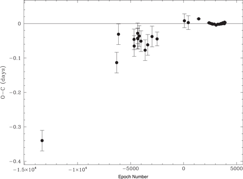
Figure 3. O–C diagram for times of the deeper eclipses of NP Per over an interval of 106 years, about 20,000 orbits. The points are shown with their estimated errors. The period has clearly changed, although during the last decade (where the observational uncertainties are all very small) the change has also been small. The current period is about 2.2285724 days, as indicated by the fitted horizontal line. The cause of the long-term and short-term variations is not known for certain, though the long-term changes might be attributed to the influence of an unseen (L3 = 0 when varied in the light curve fitting process) third component, and the short-term changes might be due to some unknown mass-loss process.
Download figure:
Standard image High-resolution imageTable 8. Observed Dates of Minimum Light for NP Per
| Typea | HJD-2400000 | Uncertainty (days) | O–C (days) | Reference |
|---|---|---|---|---|
| 1 | 18275.290 | 0.030 | −0.33990 | 1 |
| 1 | 33953.492 | 0.030 | −0.11338 | 1 |
| 1 | 34332.431 | 0.030 | −0.03093 | 1 |
| 1 | 37608.411 | 0.030 | −0.04581 | 1 |
| 1 | 37637.363 | 0.030 | −0.06519 | 1 |
| 1 | 38350.527 | 0.030 | −0.04293 | 1 |
| 1 | 38359.456 | 0.030 | −0.02821 | 1 |
| 1 | 38406.240 | 0.030 | −0.04413 | 1 |
| 1 | 38700.419 | 0.030 | −0.03610 | 1 |
| 1 | 39061.432 | 0.030 | −0.05111 | 1 |
| 1 | 39937.233 | 0.030 | −0.07731 | 1 |
| 1 | 40476.562 | 0.030 | −0.06175 | 1 |
| 1 | 41390.299 | 0.030 | −0.03761 | 1 |
| 1 | 42453.319 | 0.020 | −0.04452 | 2 |
| 1 | 48187.477 | 0.020 | 0.00816 | 3 |
| 1 | 49005.356 | 0.020 | 0.00273 | 3 |
| 1 | 51198.2779 | 0.0007 | 0.01377 | 4 |
| 1 | 53357.7485 | 0.0003 | 0.00204 | 5 |
| 1 | 53386.7202 | 0.0002 | 0.00235 | 5 |
| 1 | 53671.9751 | 0.0001 | 0.00056 | 5 |
| 1 | 54021.8587 | 0.0003 | −0.00101 | 6 |
| 1 | 54021.8589 | 0.0001 | −0.00081 | 6 |
| 1 | 54055.2868 | 0.0008 | −0.00143 | 7 |
| 1 | 54108.7723 | 0.0002 | −0.00156 | 6 |
| 1 | 54476.4860 | 0.0004 | −0.00157 | 8 |
| 1 | 54848.6540 | 0.0003 | −0.00442 | 9 |
| 1 | 55209.6845 | 0.0002 | −0.00192 | 10 |
| 2 | 55484.9086 | 0.0007 | −0.00246 | 10 |
| 2 | 55484.9116 | 0.0014 | 0.00054 | 11 |
| 1 | 55503.8555 | 0.0003 | −0.00189 | 12 |
| 2 | 55533.9424 | 0.0006 | 0.00242 | 11 |
| 1 | 55851.5139 | 0.0001 | −0.00008 | 13 |
| 1 | 55884.9413 | 0.0002 | −0.00121 | 14 |
| 1 | 55940.6570 | 0.0002 | 0.00029 | 15 |
| 2 | 56186.9104 | 0.0010 | −0.00557 | 16 |
| 2 | 56195.8284 | 0.0010 | −0.00192 | 16 |
| 1 | 56196.9427 | 0.0002 | 0.00068 | 16 |
| 1 | 56216.9989 | 0.0005 | −0.00023 | 16 |
| 2 | 56235.9476 | 0.0010 | 0.00272 | 16 |
| 1 | 56263.8011 | 0.0003 | 0.00204 | 16 |
| 2 | 56264.9188 | 0.0018 | 0.00228 | 16 |
| 1 | 56310.6001 | 0.0004 | 0.00111 | 16 |
| 1 | 56575.8011 | 0.0003 | 0.00253 | 17 |
| 2 | 56576.9207 | 0.0010 | 0.00200 | 17 |
| 1 | 56586.9412 | 0.0010 | −0.00021 | 17 |
| 1 | 56633.7454 | 0.0005 | 0.00406 | 17 |
| 2 | 56652.6908 | 0.0016 | 0.00015 | 17 |
| 2 | 56661.6048 | 0.0010 | −0.00020 | 17 |
| 1 | 56671.6305 | 0.0003 | 0.00351 | 17 |
| 2 | 56955.7795 | 0.0021 | 0.00101 | 18 |
Note.
aType 1 eclipses are the deeper eclipses, and type 2 eclipses are the shallower ones.References. (1) Kholopov (1975), (2) Diethelm (1975), (3) BRNO Contr. N. Copernicus Obs. & Planetarium, No. 31; (4) Diethelm (1999), (5) Lacy (2006), (6) Lacy (2007), (7) Hübscher & Walter (2007), (8) Agerer (2009), (9) Diethelm (2009), (10) Diethelm (2010), (11) Lacy (2011), (12) Diethelm (2011), (13) Honkova et al. (2013) (14) Lacy (2012), (15) Diethelm (2012), (16) Lacy (2013), (17) Lacy (2014), (18) Lacy (2015).
(A machine-readable version of the table is available.)
The components have a relatively short orbital period and are both rapidly rotating, thus one might expect star spot modulation, especially from the cooler component, but there is no clear evidence of spot variability in the light curve. At F5 the larger star A is likely too early in spectral type to have significant spots, and the smaller star B is possibly too faint to show a significant amplitude in the combined light.

Figure 4. Primary minima during the time the NFO was observing NP Per. The fitted curve is a parabola. The line at zero represents the linear fitted ephemeris HJD Min I = 2,455454.8289(3) + 2.2285688(6) E. The curvature shows that the orbital period is currently increasing at a rate of about 4 × 10⁻⁶ days day−1.
Download figure:
Standard image High-resolution imageThe linear ephemeris of primary eclipses during the epoch of NFO observations is given by HJD Min I = 2,455,454.8289(3) + 2.2285688(6) E. Times of secondary eclipses have a mean orbital phase of 0.50004(48), so are consistent with a circular orbit. The photometric observations in Tables 6 and 7 were analyzed by using the NDE model as implemented in the jktebop code of John Southworth (see Lacy et al. 2014 for details). Dates of observations were corrected, before analysis, for the non-linearity shown in Figure 4. The results are given in Table 9 and shown in Figures 5–7.
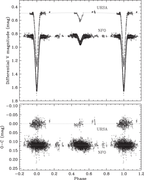
Figure 5. V-band light curves of NP Per. Residuals from the fitted orbits are shown in the lower panels.
Download figure:
Standard image High-resolution image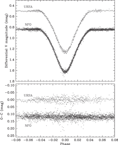
Figure 6. Primary eclipse of NP Per.
Download figure:
Standard image High-resolution image
Figure 7. Secondary eclipse of NP Per.
Download figure:
Standard image High-resolution imageTable 9. Photometric Light Curve Parameters of NP Per
| Parameters | URSA | NFO |
|---|---|---|
| (adopted) | ||
| JB | 0.2021 ± 0.0042 | 0.1829 ± 0.0073 |
| rA+rB | 0.2735 ± 0.0025 | 0.2719 ± 0.0015 |
| k | 0.867 ± 0.024 | 0.896 ± 0.014 |
| i (degrees) | 85.54 ± 0.18 | 85.431 ± 0.098 |
| uA | 0.466 fixed | 0.421 ± 0.081 |
| uB | 0.64 fixed | 0.62 ± 0.15 |
| q | 0.7916 fixed | 0.7916 fixed |
| L3 | 0 fixed | 0 fixed |
| rA | 0.1465 ± 0.0023 | 0.1434 ± 0.0016 |
| rB | 0.1270 ± 0.0024 | 0.1285 ± 0.0016 |
| LB/LA | 0.142 ± 0.038 | 0.1357 ± 0.0050 |
| LA | 0.876 ± 0.028 | 0.8805 ± 0.0012 |
| LB | 0.124 ± 0.028 | 0.1195 ± 0.0012 |
| s (mmag) | 13.56 | 13.99 |
| N | 740 | 7126 |
| Corrections | 0 | 137 |
Download table as: ASCIITypeset image
When the eccentricity and longitude of perihelion were included in the fitting as variables, the eccentricity was found to be not significantly different from zero, so circular orbits were assumed in the final fits. Because the number of NFO observations is almost 10 times the number of URSA observations, we have adopted the NFO solution to use in further analysis.
5. ABSOLUTE PROPERTIES
Accurate absolute masses and radii of the NP Per components were obtained by combining the results of the photometric and spectroscopic analyses, and are listed in Table 10. Formal errors are at the level of about 1% or smaller, on a par with some of the most precise results available for detached eclipsing binaries (Torres et al. 2010). Effective temperatures are more prone to systematic errors, and the values initially derived from our disentangled spectra were found to be somewhat sensitive to the flux ratio adopted for renormalizing them, particularly for the secondary star, which is roughly seven times fainter than the primary in the V band.
Table 10. Absolute Dimensions of NP Per
| Parameter | Star A | Star B |
|---|---|---|
| Mass (solar masses) | 1.3207 ± 0.0087 | 1.0456 ± 0.0046 |
| Radius (solar radii) | 1.372 ± 0.013 | 1.229 ± 0.013 |
| Log g (cgs) | 4.2840 ± 0.0080 | 4.2779 ± 0.0089 |
| Temperature (K) | 6420 ± 90 | 4540 ± 160 |
| Log L (solar units) | 0.460 ± 0.025 | −0.237 ± 0.058 |
| FVa | 3.805 ± 0.007 | 3.612 ± 0.009 |
| MV (mag)a | 3.53 ± 0.07 | 5.77 ± 0.23 |
| E(B–V) (mag) | 0.26 ± 0.04 | |
| m–M (mag)a | 7.34 ± 0.19 | |
| Distance (pc)a | 290 ± 25 | |
| Measured vrot sin i (km s−1) | 33.1 ± 1.2 | 32.5 ± 2.2 |
| Synchronous vrot sin i (km s−1) | 31.05 ± 0.29 | 27.82 ± 0.29 |
| [Fe/H] | 0.02 ± 0.08 | |
Note.
aRelies on the visual absolute flux (FV) calibration of Popper (1980), which is unitless. The apparent V magnitude of NP Per outside eclipse is taken to be 11.53 ± 0.11 from the APASS survey (Henden et al. 2012) and the TASS survey (Droege et al. 2006). The Tycho-2 measurement seems to be somewhat anomalous and was not used.Download table as: ASCIITypeset image
To handle this we began by estimating the temperatures from available standard photometry of the combined light in the Johnson-Cousins, Sloan, Tycho-2, and 2MASS systems (Hog et al. 2000; Cutri et al. 2003; Droege et al. 2006; Henden et al. 2012). Where possible we removed observations in eclipse to avoid biases. We constructed 14 different but non-independent color indices, and used color/temperature calibrations by Casagrande et al. (2010) and Huang et al. (2015) to infer mean effective temperatures. Solar metallicity was assumed, in accordance with our measurements reported in Section 3, and the colors were de-reddened by adopting E(B–V) = 0.26 ± 0.04 based on the recent extinction map of Green et al. (2015), and a preliminary distance estimate of 300 pc. We note that this level of reddening is considerably higher than estimates from earlier sources (Burstein & Heiles 1982; Hakkila et al. 1997; Schlegel et al. 1998; Drimmel et al. 2003; Amores & Lepine 2005), but is consistent with independent estimates by Belikov et al. (2002b) for stars in the same region as NP Per and at the same distance. The resulting mean photometric temperature, 6070 ± 180 K, was combined with the value of the central surface brightness ratio from our JKTEBOP solution (Table 9) and with the visual absolute flux calibration of Popper (1980) to infer preliminary individual temperatures for the components (approximately 6400 and 4550 K for the primary and secondary).
Synthetic spectra based on PHOENIX model atmospheres (Husser et al. 2013) for those temperatures were then used to estimate the flux ratio as a function of wavelength. This served in turn to renormalize the disentangled spectra and produce more reliable spectroscopic estimates of the temperatures. This process was iterated once more, resulting in the final flux ratio as a function of wavelength displayed in Figure 8, and final adopted spectroscopic temperatures of 6420 ± 90 K and 4540 ± 160 K, as reported earlier in Section 3. These correspond to spectral types F5 and K5, respectively. The excellent agreement between the predicted flux ratio integrated over the V band (indicated with a square in Figure 8) and the value measured from the light curve fit (cross) is an indication that the spectroscopic and photometric analyses are self-consistent, and supports the accuracy of the radius ratio from the light curve. We note also that the spectroscopic temperature difference (1880 ± 180 K) is in good agreement with the more precise value expected from the central surface brightness ratio (1840 ± 70 K). The weighted average projected rotational velocities from our two determinations, also listed in Table 10, are slightly larger than synchronous rotation. The uncertainties in the measured v sin i values are conservative estimates. Phase smearing during the 60 minutes spectroscopic observations could broaden the lines, at the most, by 0.5 km s−1, so the actual v sin i values are likely smaller and closer to the synchronous rotation values.
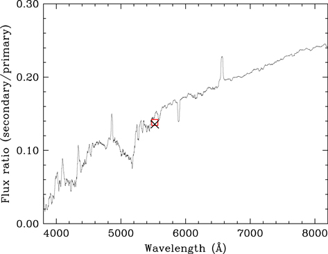
Figure 8. Flux ratio as a function of wavelength between the secondary and primary of NP Per computed from solar-metallicity PHOENIX spectra (Husser et al. 2013) for temperatures near our final values. A smoothed version of this relation was used for renormalizing the disentangled spectra. The square represents the predicted flux ratio in V, and the cross is the measured value from the NFO light curve.
Download figure:
Standard image High-resolution image6. COMPARISON WITH STELLAR EVOLUTION MODELS
The accurate properties derived for NP Per and its status as a very young binary illustrated below provide a unique opportunity to test models describing the early stages of stellar evolution. In Figure 9, we compare the observations against evolutionary tracks for solar metallicity and masses near those we measure for each component, computed using the MESA code (Modules for Experiments in Stellar Astrophysics; Paxton et al. 2011, 2013, 2015) and interpolated from an extensive grid of models presented by Choi et al. (2016).
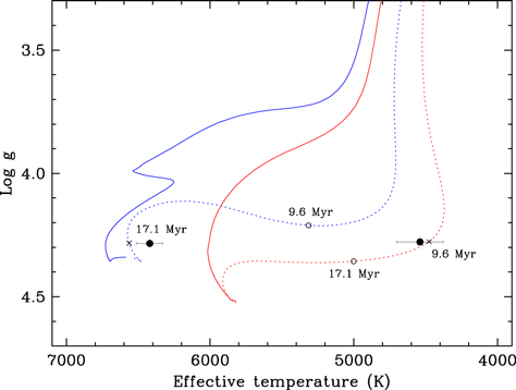
Figure 9. MESA evolutionary tracks for solar metallicity and masses of 1.32 (blue) and 1.04 solar masses (red) compared against the measured log g and temperature of the NP Per components. PMS sections of the tracks are indicated with dotted lines, which are changed to solid when they reach the main sequence. The beginning of the main sequence is defined in these models as the point where the hydrogen-burning luminosity exceeds 99.9% of the total luminosity before the central hydrogen fraction falls below its initial value by 0.0015 (see Dotter 2016). The small crosses on the tracks are placed at the best-fit age for each star, and the open circles mark the location of each component at the best-fit age for the other star.
Download figure:
Standard image High-resolution imageThe cooler secondary is clearly in the PMS stage (dotted section of the evolutionary tracks) near the bottom of the Hayashi track, while the primary, also a PMS star, is close to the end of the radiative phase approaching the zero-age main-sequence (ZAMS). The agreement between theory and observation appears fairly good in this diagram, with the temperature of the primary being only marginally cooler than expected by about 1.5σ. However, there is in fact a rather serious hidden discrepancy in that the inferred age of the primary based on its size is 17.1 ± 0.2 Myr, while that of the secondary is only 9.6 ± 0.6 Myr. Tests with different sets of models from the Dartmouth (Dotter et al. 2008), PARSEC (Bressan et al. 2012) and Pisa series (Tognelli et al. 2011) produce qualitatively similar results, always suggesting the secondary is significantly younger than the primary.
The discordance is shown more directly in Figure 10, where the predicted radius and temperature of both stars are given as a function of age. To our knowledge no compelling evidence has been presented of real age differences among close binary components that cannot be ascribed to observational errors (see, e.g., Valle et al. 2016 for a recent discussion of the influence of empirical uncertainties on ages, and also Kraus & Hillenbrand 2009)6 . If we make the assumption that the true age of the system is closer to the age of the primary star, then the measured properties of the secondary are in significant disagreement with theoretical predictions for that age: the secondary appears too large as well as too cool for the measured mass (see Figure 10, and also Figure 9). The direction of these differences is reminiscent of that found in many well-studied main-sequence eclipsing binaries with cool components, a phenomenon that is thought to be related to stellar activity (see, e.g., Torres 2013). The opposite assumption, that the binary has the age inferred for the secondary, seems less likely as it would imply an enormous temperature discrepancy for the primary of more than 1000 K.

Figure 10. Radius, temperature, and Li abundance on the scale of Asplund et al. (2009) for the NP Per components as a function of time (solid lines for the primary, dashed for the secondary), according to the same MESA models from Figure 9. The observations for the primary and secondary are shown with filled symbols at the age that best fits the radius of each star (dotted lines). The secondary properties arbitrarily shifted to the older age of the primary are represented with open symbols. Crosses indicate the age of arrival on the ZAMS.
Download figure:
Standard image High-resolution imageOur measurement of the Li abundance for the primary, shown in the lower panel of Figure 10, is consistent with predictions from the MESA models within the error. The secondary, however, seems somewhat less depleted than expected by about 2 sigma at the nominal secondary age and almost 3 sigma at the age of the primary. This discrepancy is in the same sense as pointed out by Choi et al. (2016), who noted that standard models even fail to match the Li depletion in the Sun, a star not very different in mass from the secondary of NP Per. Models tend to burn too much lithium early on, clearly indicating some missing physics. Possibilities suggested by Choi et al. (2016) include rotation during the PMS stage (not incorporated into these models), or changes in the mixing length parameter.
7. DISCUSSION AND FINAL REMARKS
NP Per is included in a catalog of some 30,000 stars in the region of the Perseus star-forming region compiled by Belikov et al. (2002a) on the basis of astrometric and photometric information. The binary is very likely associated with the Per OB2 association embedded in the complex. This is supported by the kinematics of NP Per (Tycho-2 proper motion; Hog et al. 2000) matching those of stars in the association, our distance estimate of 290 pc in excellent agreement with estimates for Per OB2 by Belikov et al. (2002b), 270–320 pc, and the high lithium abundance, particularly for the secondary. The comparison with stellar evolution models in the preceding section confirms its youth, which is also broadly consistent with estimates for other stars in the association.
The importance of NP Per stems from the fact that it is one of relatively few known PMS double-lined eclipsing binaries that are amenable to detailed investigations such as ours. These systems are critical for testing stellar evolution models at young ages, which are largely unconstrained by observations. Studies of only 15 such binaries have appeared in the literature to date (see Stassun et al. 2014, Kraus et al. 2015, Lodieu et al. 2015), though only four of them have absolute masses and radii measured to better than 3%. NP Per now joins that group.
The disagreement between theory and observation for NP Per in the log g versus temperature diagram is intriguing. It is seen in all models, suggesting a common problem with the physical ingredients. Under our working assumption that the binary system has the age of the primary, the secondary appears both larger and cooler than predicted by the MESA models by about 9% in each quantity. Similar degrees of "radius inflation" and "temperature suppression" observed in many well-measured M dwarfs (or more generally any star with a convective envelope) that are members of eclipsing binaries are ascribed to magnetic activity and/or spots, which are not included in standard models. Our SPD enables us to investigate this idea. While the reconstructed spectra are too weak in the blue to check for the possible presence of emission cores in the Ca ii H and K lines, the disentangled spectrum of the secondary in the Hα region shows that this line is filled in by emission up to the level of the continuum (see Figure 11), indicating a significant level of chromospheric activity, as would be expected for a very young and rapidly rotating K star. Spots are also likely on this star, although as pointed out earlier any light curve modulation by spots would be difficult to detect given the flux ratio of about 7 in the V bandpass.

Figure 11. Section of the disentangled spectrum of the secondary of NP Per (blue) showing the Hα line filled in compared to a model for the properties of that star (red).
Download figure:
Standard image High-resolution image
Activity effects have been discussed specifically for PMS stars by Stassun et al. (2014) and also Somers & Pinsonneault (2015). The former authors examined the impact of activity on the theoretical predictions for their sample of 13 PMS eclipsing binaries, many of which are also not well fit by models, but concluded that activity alone was not able to fully explain the discrepancies. In noting that many of their systems are triples, they proposed that the influence of third components may also partially explain some cases through dynamical or tidal interactions and ensuing heat transfer between the wide companion and one or both stars in the inner pair, which could change their global properties. Tokovinin et al. (2006) showed that the fraction of close binaries with additional companions is as high as 96% for binary periods under 3 days. Given its orbital period of 2.2 days, it would therefore not be surprising if NP Per turned out to be triple. Although there is no evidence of a third star in our spectra, in the velocity residuals, or from our light curve analysis (L3 = 0), the eclipse timings do show clear deviations from a linear ephemeris (Figures 3 and 4) that may well be caused by a wide companion, but could also have a different origin.
NP Per is an important PMS binary worthy of further study. A better determination of the Li abundance for the faint secondary would be helpful. We encourage also deeper searches for additional components in the system, such as by high-resolution imaging or higher signal-to-noise spectroscopy.
The authors wish to thank Dr. A. W. (Bill) Neely who operates and maintains the NFO WebScope for the Consortium, and who handles preliminary processing of the images and their distribution. The research at Tennessee State University was made possible by NSF support through grant 1039522 of the Major Research Instrumentation Program. In addition, astronomy at Tennessee State University is supported by the state of Tennessee through its Centers of Excellence programs. The work of K.P. has been supported in part by the Croatian Science Foundation under grant 2014-09-8656. We are very grateful to Jieun Choi (Harvard University) for providing the MESA evolutionary models used here and for clarifying some details of those calculations, as well as to Arne Henden (AAVSO) for providing the epoch photometry for NP Per. G.T. acknowledges partial support for this work from NSF grant AST-1509375.
Footnotes
- 6
The one possible exception is the case of Par 1802 (Stassun et al. 2008), a very cool and much younger (∼1 Myr) eclipsing binary than NP Per in the Orion Nebula, which shows somewhat different measured component temperatures and radii despite having nearly the same mass (0.4 solar masses). At these very young ages, some models predict very rapid evolution of the stellar properties such that a lag of a few hundred thousand years in their age could explain their different properties. However, these differences would only be observable for very young systems such as Par 1802; subsequent evolution over the next few Myr would soon erase them, and the stars would appear coeval within measurement uncertainties.