
Abstract
We report on an experimental investigation of the jitter of electrons from laser wakefield acceleration. The relative arrival timings of the generated electron bunches were detected via electro-optic spatial decoding on the coherent transition radiation emitted when the electrons pass through a 100 μm thick stainless steel foil. The standard deviation of electron timing was measured to be 7 fs at a position outside the plasma. Preliminary analysis suggested that the electron bunches might have durations of a few tens of femtoseconds. This research demonstrated the potential of laser wakefield acceleration for femtosecond pump–probe studies.
Export citation and abstract BibTeX RIS

Content from this work may be used under the terms of the Creative Commons Attribution 4.0 license. Any further distribution of this work must maintain attribution to the author(s) and the title of the work, journal citation and DOI.
Laser wakefield acceleration (LWFA), 1–4) as an advanced accelerator concept, has invoked great interest worldwide due to the inherent nature of the femtosecond (fs) time scale and high acceleration gradient. With the rapid development of the chirped pulse amplification (CPA) technique, 5) laser pulses with durations of a few tens of femtoseconds and powers over a terrawatt (TW, 1 TW=1012 W) are commonly implemented in laboratories around the world. By the incidence of such femtosecond high-power lasers into underdense plasma, electron plasma waves with electric field strengths over 100 GeV m–1 can be generated, allowing the trapped electrons to achieve kinetic energies over GeV within centimeters. Milestone results of quasi-monoenergetic electron beams with energy over GeV 6,7) or relative energy spread smaller than 1% 8) were achieved. In particular, free-electron-lasing at 27 nm driven by LWFA was demonstrated recently. 9) Such a compact femtosecond secondary X-ray source is believed to have potential in the application of ultrafast pump–probe studies for physics, chemistry, biology, material science, and industries.
For the ultrafast pump–probe study, the time resolution is partially determined by the duration and jitter of the probe pulse. In the case of LWFA, the probe X-ray pulses are generated via the secondary oscillation processes of electron bunches inside a plasma channel 10,11) or an external undulator. 9,12) With the acceleration structure of typically less than a few tens of micrometers, it is reasonable to assume that the electrons and thus secondary X-ray sources from LWFA have bunch durations of fs 13) to tens of fs level.
The electron bunches from LWFA were always assumed to be trapped in the first bucket of the plasma wave just after the drive laser. Thus, the electron jitter issue in LWFA was always neglected. However, for linear plasma waves, 14) the wakefields extend to several hundreds of micrometers. The possibility of random injections of electrons into lateral wave buckets should not be ignored. For application concerns, when generating the secondary X-ray source via an external undulator, the electron timing at a position outside the plasma is of great importance since it shows the jitter of the X-ray source. Nevertheless, experimental single-shot detections of the timings of laser wakefield accelerated electrons outside the plasma had barely been conducted.
Electro-optic (EO) sampling is a convenient technique for the measurement of terahertz (THz) pulse duration 15) and was introduced to accelerator study for the investigation of temporal information of electron bunches. 16–28) When the electric field carrying the longitudinal information of the electron bunch passes through the EO crystal, the effective optical axis of the crystal rotates and birefringence will occur. The polarization of a linear polarized probe laser becomes elliptical due to phase retardation, which can be used to reconstruct the original temporal distribution of the electron bunch. Usually, there are two ways of generating the signal electric field: one is to directly detect on the Coulomb field of the electron bunch; 27,29–31) the other is to generate coherent transition radiation (CTR) pulses by inserting a thin metal foil in the electron path. 28) By setting a relative angle between the probe laser and the signal field, the longitudinal distribution of the electron bunches is encoded to the transverse intensity profile of the probe laser. This is the so-called EO spatial decoding technique. 27) When the signal electric field is incident normal to the crystal surface, there is a temporal mapping relationship: 27,29)

where Δτ is the timing difference, Ψ is the relative angle between the probe laser and electron path, Δξ is the displacement observed by CCD and c is the speed of light in vacuum.
In this paper, we report on the measurement of relative electron timing in LWFA. By imaging the CTR emitted when the electron bunch passes through a metal foil to a Gallium Phosphide (GaP) crystal, we achieved a temporal resolution of 1.6 fs via the EO spatial decoding technique. By using a supersonic nozzle with hydrogen (H2)-nitrogen (N2) mixture gas, the standard deviation of electron arrival timing was measured to be 7 fs at a position 7 cm away from the exit of the plasma. Preliminary calculations suggested that the electron bunches should possess a duration of a few tens of femtoseconds.
The experiment was performed at the LAPLACIAN (Laser Acceleration Platform as a Coordinated Innovative Anchor) platform at the RIKEN SPring-8 Center. The laser system had delivered two Ti:Sapphire laser beamlines with powers up to 40 TW (BL1) and 80 TW (BL2) at a center wavelength of λ0=800 nm. The BL1 and BL2 shared the same front end. Yet, they were equipped with separated final amplifiers and pulse compressors, allowing experimental conditions of various laser pulse durations and powers. In our experiment, the BL1 was used as a probe laser without final amplification. The BL2 was used as a drive laser and had a pulse duration of 30 fs and power of 50 TW on target. The experimental setup is illustrated in Fig. 1(a). The drive laser was focused by an F/20 off-axis-parabolic (OAP) mirror to a supersonic gas nozzle for electron generation. The focal spot had a size of 25 μm × 22 μm (FWHM) and intensity of 5.8 × 10¹⁸ W cm– 2, corresponding to a normalized vector potential a0 ∼ 1.65, where a0 = 8.6 × 10⁻¹⁰ λ0[μ m] I1/2 [W cm– 2]. 14) The CTR was generated by inserting a 100 μm stainless steel (SUS) foil at a distance of 7 cm after the exit of the gas jet and then collected and imaged by two gold-coated OAPs (OAP1 and OAP2) to the GaP crystal with a magnification of 1. Both OAPs had a diameter of 50.8 mm and a focal length of 190 mm. The energy spectra of scattered electrons after OAP1 were recorded using the electron energy spectrometer (ESM). The probe laser was delivered by silver mirror with ultra-low group delay dispersion at 800 nm.
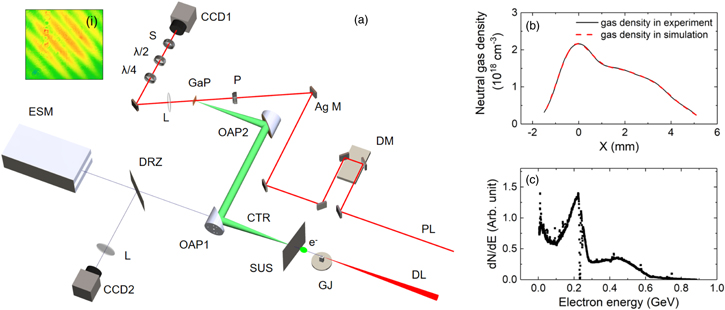
Fig. 1. (Color online) (a) Experimental set-up. DL: Drive laser; PL: Probe laser; GJ: Gas jet; e−: electron bunch; SUS: 100 μm stainless foil; OAP: Off-axis-parabolic gold mirror; DM: Delay module; Ag M: Ag mirror; DRZ: Gd2O2S: Tb phosphor screen (Mitsubishi Chemical, DRZ-High); CCD: Charge-coupled device; ESM: Energy spectrometer; L: Lens; GaP: Gallium Phosphide crystal with a thickness of 100 μm; P: Polarizer; λ/2: Half waveplate at 800 nm; λ/4: Quarter waveplate at 800 nm. The distance between the SUS to the exit of the gas jet was 7 cm. The SUS was slightly tilted to avoid light reflection back into the laser system; (b) The density profile of the gas jet. The black curve shows the profile measured by a Mach-Zehnder interferometer. The red dashed line is the density profile used in simulation; (c) is an electron energy spectrum. The speckles and discontinuities in the data were caused by gamma-ray noise and ESM set-up in the experiment. The inset (i) in (a) is an interferometry pattern when adjusting the timing difference between the DL and PL.
Download figure:
Standard image High-resolution imageTo perform EO spatial decoding, the probe laser, with pulse duration the same as the drive laser, was introduced to the (110) cut GaP crystal with an incident angle of Ψ =2 7°. The GaP crystal had a thickness of 100 μm and was placed at the focal plane of the OAP2. The incident probe laser had polarization at the horizontal (P) direction and along the [-1,1,0] axis of the GaP crystal. For spatial and temporal alignment, the drive laser in a low-energy mode was used as a simulation light of CTR and was delivered by OAP1 and OAP2 to the position of the GaP crystal. An interferometry pattern was generated when the timing of both lasers were well adjusted, as illustrated in the inset of Fig. 1(a). The imaging point was below the center of the CTR focus of OAP2 , as shown by the tilted line pattern in the inset figure. A polarizer in the vertical (S) direction was placed before the CCD1 in a cross-polarization set-up. For the electron timing detection, the relative angles of λ/4 and λ/2 waveplates were set to be zero, as shown in Fig. 1(a). Limited by the imaging system, the temporal resolution of the electron arrival timing measurement was 1.6 fs, which was measured by setting the probe delay at 5 different timings. Since the arrival timing measurement only concerns the center position of the EO signal, the temporal resolution here was basically limited by the EO imaging system.
For the stable generation of electron beams, the gas reservoir pressure was precisely controlled via a digital controller (General Electric, Dr.uck PACE5000). The gas nozzle was designed to have a density peak at the entrance followed by a mild long density down-ramp, illustrated as the black curve in Fig. 1(b). Two kinds of gases were utilized: one is pure hydrogen gas, the other is a mixture gas composed of 99% hydrogen (H2) and 1% nitrogen (N2). The electron results showed that the pure H2 gas worked at higher gas pressure for the injection to happen, while the mixture gas had better stability in aspects of pointing and occurrence of collimated electron beams even at a lower plasma density. Relatively stable electron beams were generated with the mixture gas at a pressure of 0.65 MPa, corresponding to a peak neutral gas density of 2.16 × 1018 cm−3. At this condition, collimated electron beams were generated every shot and the pointing fluctuation was <2 milliradian (mrad) (rms) recorded by CCD2. By inserting the OAP1 and SUS, CTR was generated and the EO signal was detected. A consecutive 34 shots of EO signals were plotted out in Fig. 2(a). We observed that the timing fluctuation at 0.65 MPa was quite small. By Gaussian fitting to the EO signals, the center positions were listed in Fig. 2(b). The electron timing fluctuation had a standard deviation of merely 7 fs. Noted that the signals in Fig. 2(a) had intensity variations, which could be a result of the fluctuations of the charges and energies of the electron bunches.
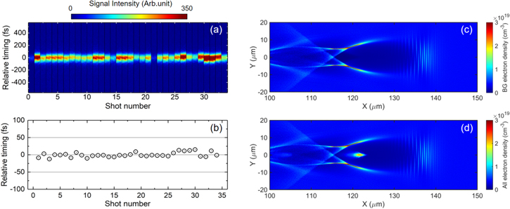
Fig. 2. (Color online) Electron bunch arrival timing measurement and injection process analysis. (a) is the EO raw data. The signal intensity fluctuation in figure should be a result of electron beam charge and energy variation shot by shot. (b) illustrates the center timings by Gaussian fitting. The relative "zero" timing was defined by the mean timing. (c) and (d) are the 2D density distribution of the background electrons and all electrons (including K-shell ionized electrons) from a 2D PIC simulation. The data was plotted out at a laser propagation time of 6.4 picosecond (ps). The color scales are set to be the same.
Download figure:
Standard image High-resolution imageIn our previous work with a moderate drive laser intensity (4 × 10¹⁷ W cm– 2, a0=0.57), 30) the relative emission times of electron bunches had quite large fluctuations due to uncontrolled self-injection. We had suggested using a controllable injection mechanism to achieve minimum jitter. Just as our prediction, with the effort of the design of gas profile, mixture gas, and a relativistic drive laser (a0 = 1.65 > 1), electron bunches with jitter of femtosecond scale were generated in this experiment.
To qualitatively investigate the electron injection process, a 2-dimensional (2D) particle-in-cell (PIC) simulation was performed using the code EPOCH. 32) The laser parameters were set to be similar as those in the experiment. The gas density profile in the simulation is illustrated by the red dashed line in Fig. 1(b). The moving window had a size of 160 μm × 100 μm and cell numbers of (Nx , Ny ) = (5120, 1250). The first 5 L-shell electrons of the nitrogen atom were set to be pre-ionized due to a much lower ionization threshold than K-shell electrons. Ionization injection occurs when the K-shell electrons are ionized near the peak of the laser field and satisfy the condition: ϕf − ϕi < − me c2/e, where ϕf and ϕi are the final and initial wake potential the electron feels. 33) Since the K-shell electrons feel a much higher ϕi when born, ionization injection occurs typically easier than self-injection. The electron density 2D distributions were plotted as Fig. 2(c) (background electrons) and (d) (all electrons including K-shell ionized electrons). From Fig. 2(c), we found there were no injections of the background electrons. Yet, a clean electron bunch from ionization injection of nitrogen K-shell electrons can be found in the first period of the wake wave, as shown in Fig. 2(d). The injection of electrons works in a relatively controlled way at this plasma density, which is in correspondence with the extremely small timing fluctuation in Fig. 2(a) and (b). For the stable generation of electron beams, we need to work at a lower plasma density to weaken various plasma instabilities. Although we had a down-ramp at the beginning of the nozzle, the injection of background electrons did not occur with a low plasma density because the density profile was not steep enough, as shown in Fig. 1(b). To trigger the injection, the mixture gas was used. Though 2D PIC simulations have discrepancies with the 3-dimensional (3D) case on the aspects of laser self-focusing, electron injection, and total electron charge, this numerical analysis suggested that clean electron bunches could be generated in our experiment with well-controlled gas pressures and species.
Although the jitter of our electrons was quite small, it is still important to consider the reasons why there was still a timing fluctuation of 7 fs. Several possible factors could be responsible: (1) The electron pointing fluctuation. With a SUS distance of 7 cm, electron bunches with a pointing fluctuation of 2 mrad will result in a travelling time difference of 0.43 fs (0.14 μm); (2) The electron energy fluctuation. As shown in Fig. 1(c), the electrons had energies covering a wide range. Actually, the energies of the electron bunches fluctuated in the experiment. The fluctuation of electron energy could cause travelling time lag of tens of femtoseconds from the gas jet to the SUS screen; (3) The relative jitter between the probe laser and drive laser. Although the probe laser and drive laser shared the same laser front end in our system, they were delivered separately over tens of meters with many optics that could cause pointing fluctuation due to vibrations. This factor should be characterized carefully in the near future; (4) The fluctuation of electron pulse duration. The change in electron pulse durations will cause fluctuations in frequency compositions and thus different group velocities of the CTR in the EO crystal. 31) (5) Existed plasma wave bucket size. Figure 2(d) suggested a bucket size of around 20 μm, i.e. 66 fs. The fluctuations in laser intensity and gas profile can cause the injection of the electrons to be earlier or later. Even within the same bucket, the center positions of the electron bunches could still have a timing variation of tens of femtoseconds.
The timing measurement above was performed in a cross-polarization set-up where the signals were proportional to E2 CTR . Although exact bunch shape cannot be measured in such a set-up, the detection of center timing of the electron bunch was not affected. 23,30)
Next, for the estimation of the upper limit of the electron bunch duration, the λ/2 plate was set to an angle of θ = 2° to perform a near-cross-polarization measurement. The λ/4 plate was tuned to diminish the residual birefringence caused by the EO crystal. The signal was almost linear
25) with respect to the original CTR field when the phase retardation was small, i.e.  . The signal was processed with two backgrounds as: Isig = (Iraw − B2)/(B2 − B1), where B2 was the background with laser but no gas, B1 was the dark image with no laser and no gas. The raw signal can be described as
 ![${I}_{{\rm{raw}}}={I}_{{\rm{probe}}}[1-\cos ({\rm{\Gamma }}+4\theta )]/2+{\delta }_{{\rm{ext}}}{I}_{{\rm{probe}}}+{B}_{1}$](https://content.cld.iop.org/journals/1882-0786/15/3/036001/revision3/apexac5237ieqn2.gif) ,
25) where Γ is the phase retardation, Iprobe is the probe laser intensity and δext = 1.25 × 10⁻⁵ is the extinction ratio
30) of the polarizer pair. With laser but no gas (Γ = 0),
,
25) where Γ is the phase retardation, Iprobe is the probe laser intensity and δext = 1.25 × 10⁻⁵ is the extinction ratio
30) of the polarizer pair. With laser but no gas (Γ = 0), ![${B}_{2}={I}_{{\rm{probe}}}[1-\cos (4\theta )]/2+{\delta }_{{\rm{ext}}}{I}_{{\rm{probe}}}+{B}_{1}$](https://content.cld.iop.org/journals/1882-0786/15/3/036001/revision3/apexac5237ieqn3.gif) . Thus, the signal after processing is derived as:
. Thus, the signal after processing is derived as:

Equation (2) can be used to calculate the achievable signal shape for estimation and fitting. A calculation code has been developed covering the overall signal generation process from the electron bunch profile to EO signal, which includes: CTR generation, CTR imaging, broadening introduced by probe laser pulse duration, EO crystal thickness, EO crystal dispersion, the smearing between the probe laser and the CTR field inside the crystal and the elongation of probe laser after propagating through the crystal. The detailed elaboration of this calculation method will be published elsewhere.
The line-out in Fig. 3(a) illustrates a typical shot of near-cross-polarization measured Isig. A direct Gaussian fitting of the main peak results in a duration of 40 fs (rms). Note that this value is not the exact original electron bunch duration. Oscillations can be observed in the signal. Such oscillations are the results of absorption and dispersion of the CTR field inside the EO crystal when the field possesses a duration of less than a few tens of femtoseconds. For the rough estimation of the upper limit of the electron bunch duration, a single Gaussian electron pulse shape is assumed. A calculation of the EO signal shapes for original electron bunch duration of 20 fs, 30 fs, 50 fs, 100 fs (rms) is conducted, as shown in Fig. 3(b). These temporal line-out plots are calculated at a position (x, y)=(1000 μm, 1000 μm) (x and y are the horizontal and vertical coordinates) from the center of the CTR field. For a bunch duration larger than 50 fs, there are no such oscillations, indicating the high-frequency part of the CTR field has been cut off by the long bunch duration. For a bunch duration of 30 fs, mild oscillations appear. When the bunch duration is shorter than 30 fs, strong oscillations and distortions appear due to the absorption and phase mismatch of the high-frequency components. Since strong oscillations can be found in the experimental data, it is conservative to estimate that the electron beams had a bunch duration smaller than 50 fs, i.e. few tens of femtoseconds. This estimation is consistent with the bubble size of ≈20 μm, as illustrated by the simulation results in Fig. 2(c) and (d). The parameters chosen in the calculation are just for estimations. We have performed calculations at other positions with various distances to the center of the CTR field. Such oscillations start to appear at similar bunch durations. Although this is not an exact fitting of the original bunch shape, it demonstrates the upper limit of the possible bunch durations in our experiment. Note that the negative parts in Fig. 3(a) are not noticeable enough. One of the reasons might be the subtraction of the background was not clean enough.

Fig. 3. (Color online) Estimation of the upper limit of the electron bunch duration. The line-out in (a) denotes the experimental signal in a near-cross-polarization measurement. (b) illustrates the calculated signal shapes for original electron bunches with r.m.s. durations of 20 fs (green), 30 fs (black), 50 fs (red), 100 fs (blue). All the plots in this Fig. use normalized intensities.
Download figure:
Standard image High-resolution image
Since the Coulomb field of the electron bunch has an opening angle, with a longer distance from the center of the CTR field to the observation point, the duration of the field is broader. To detect the field structures at various distances for the exact reconstruction of the electron bunch shape, the center of the CTR should be aligned into the view window of CCD1 in Fig. 1. Those experiments will be conducted soon. In this paper, we do not intend to measure the exact longitudinal distribution of the electron bunch. The elaboration based on Fig. 3 is aimed to estimate an upper limit of electron bunch duration. For electron bunch durations >50 fs, the signal oscillation in Fig. 3(a) should not have appeared.
In conclusion, a single-shot electron temporal measurement was conducted at the LAPLACIAN platform. Via EO spatial decoding on the CTR generated by the laser wakefield accelerated electron beam at a position outside the plasma, electron timing fluctuation of merely 7 fs was observed when working in a controlled injection regime. By estimation using simple models, the electrons were discovered to have bunch durations of a few tens of femtoseconds. The research showed the capability of the EO technique as a real-time diagnostic for the electron temporal information in LWFA and demonstrated the ultrafast and extremely small-jitter nature of laser wakefield accelerated electron bunches.
Acknowledgments
We are grateful for the encouragement from Dr. Y. Sano, and Dr. N. Kumagai. We thank Prof. R. Kodama for the construction of the LAPLACIAN platform. We acknowledge the technical assistance from Dr. I. Daito and Dr. Y. Sakai. This work was funded by the JST-Mirai Program Grant No. JPMJMI17A1, Japan, the Grant-in-Aid for Early-Career Scientists (No. JP21K17998) from JSPS KAKENHI, Japan and the QST President's Strategic Grant (Exploratory Research), Japan.