
Abstract
Many photovoltaic (PV) systems are connected to electrical power grids, and the grids are at risk of instability due to fluctuation of PV output. Numerical weather prediction (NWP) models are used to forecast solar irradiance and proper grid management. NWP usually has many physical parameterization options, and appropriate schemes of these options should be selected for accurate forecasting. The options should be determined by regional and climatic conditions and other factors. The target country is Thailand, which is in the tropics. In Thailand, cumulus and cumulonimbus clouds frequently appear, and their behavior makes weather forecasting difficult. The optimal combination of schemes in the tropics is determined through a sensitivity analysis of the options. By the optimization the forecasting accuracy increases from 0.773 to 0.814 of the correlation coefficient. It is also found that surface layer and PBL processes make a significant contribution to the improvement of accuracy.
Export citation and abstract BibTeX RIS
1. Introduction
Nowadays, a huge number of photovoltaic (PV) systems are widely used and connected to electrical power grids. PV systems have become one of the major sources for grids in some countries. In Germany, PV systems provided 6.5% of nationwide electricity consumption in 2013 1) and the rate increased to 8.6% in 2019. 2) The PV penetration in national electricity supply reached more than 8.0% in 2019, not only in Germany but also in five other countries, two of which are Honduras (14.8%) and Israel (8.7%). 2) Under the circumstances, the supply by PVs regularly covered about one-third of the noon peak demand on sunny summer days in Germany in 2013. 1) However, their output is not stable due to weather change and solar irradiance fluctuation, and this causes the risk of instability in the electrical power supply from the grids.
In Thailand, which is the target area of this study, the national government promotes the installation of large-scale PV power plants to manufacture PVs as a major electrical power source to shift to renewable energy in order to create a sustainable society. EA Solar Phitsanulok plants with 133.92 MWp and EA Solar Lampang plants with 128.39 MWp 3) are currently operating. Some of the electrical power is also exported to the neighboring countries. The fluctuation in electrical power supplied from large PV power plants is more serious than that distributed from household PV systems, because no smoothing effect in space 4,5) is expected.
One of the ways to reduce the risk and efficient management of grids with PV systems, is forecasting of solar irradiance, which is related to PV output that is employed for the management of the grids. Diagne et al. 6) reviewed the reliability of solar irradiance forecasting with statistical models, cloud imagery and numerical weather prediction (NWP) models, and showed the advantage of NWPs. Heinemann et al. 7) also investigated two kinds of forecasting; image processing for cloud development for very short-period forecasting and NWP for up to two days, and indicated the validity of a combination of NWP and post-processing for solar irradiance forecasting. Lorentz et al. 8) employed weather forecasting provided by the European Centre for Medium-Range Weather Forecasts for solar irradiance and PV power predictions, and used this information for electrical grid management in Germany. Their forecasting period is three days. They also discussed the so-called "area size effect", which is the smoothing effect by space averaging the solar irradiance in different area sizes to reduce forecasting error. Lara-Fanego et al. 9) forecasted solar irradiance using NWP in southern Spain. They evaluated not only global horizontal irradiance, but also direct normal irradiance by introducing physical post-processing of the NWP. Shimada et al. 10) also performed solar irradiance forecasting in Japan with the same NWP as Lara-Fanego et al., 9) and obtained results with lower accuracy than Lara-Fanego et al. They pointed out that the low accuracy in forecasting the Japanese weather conditions is because Japan is less sunny and more cloudy compared with southern Spain, and the weather changes frequently, which together make it difficult for forecasting. Aryaputera et al. 11) also use an NWP to forecast the irradiance in Singapore in the Southeast Asia region, which is near the target area, Thailand, in this study. They also proposed stochastic methods, and improved the forecasting accuracy by coupling the results from the NWP and the methods.
The authors have constructed a weather and solar irradiance forecasting system for the prediction of PV generation and its fluctuation, 12) and are monitoring the management of the electrical power grid to which the large PV power plants are connected. For effective management, high accuracy forecasting is required. However, the target area, Thailand, is in the tropical monsoon region and the weather changes suddenly, especially in the rainy season.
The weather in Thailand is divided into three seasons. The first is the rainy season from mid-May to October. The air is wet and warm, and squalls frequently occur. Winter is from November to mid-March, during which the weather is dry with mild temperatures. Summer is from mid-March to mid-May, and the weather is very hot. It is said that weather forecasting in the tropics is relatively more difficult than in the temperate (middle) latitude zone, such as Japan. 13,14) Clouds and rainfall in the temperate latitudes are due to the frontal development of air mass, the movement of which is gradual. Therefore, forecasting in the latitudes is very reliable and easy. On the other hand, in the tropics convectional clouds and rainfall occur due to thermally induced low-pressure systems. Their movement is vertical and fast, and they make forecasting of the weather phenomenon in the tropics difficult. Cumulus and cumulonimbus clouds are common in the tropics, and their behavior, especially their generation, is complicated and difficult to forecast. This makes it difficult for solar irradiance forecasting and the prediction of PV generation in the tropics.
Climates around the world vary widely, e.g. tropical, temperate and arctic zones. NWPs cannot reproduce them perfectly due to their imperfections. The imperfections of input data as initial and boundary conditions are also a factor in the degradation of computational results. An NWP is constructed with a core model, which is indicated by the governing equations of fluid dynamics and sub-models, which are called parameterization options. The parameterization options reproduce various weather phenomena, such as rainfall and cloud generation. Various schemes are available for each option, and appropriate schemes are selected and used for accurate weather forecasting according to the target meteorological parameter, target region and other computational conditions. 15,16) Baki et al. 17,18) Chinta et al. 19,20) Di et al. 21) and Mohanty et al. 22) mentioned the impact of the different meteorological data used as initial and boundary conditions of the simulation to the simulation results and their accuracy, and pointed out that the performance of NWP models depends on the quality, reliability and representativeness of the initial values and lateral boundary conditions. 22) Consequently, seeking the appropriate combination of schemes for the parameterization option is important.
Seeking the appropriate combination of schemes is performed and reported by researchers and operators of weather forecasting. Arasa et al. 15) performed NWP computations repeatedly by changing schemes of six parameterization options, and found their optimal combination for weather forecasting in southern Spain. Their objective variable is wind on the ground, but temperature and relative humidity on the ground are also improved by the optimization. They pointed out the importance of setting appropriate schemes by showing the improved accuracy of the forecasting with the optimal combinations. The targets of Baki et al. 17,18) Di et al. 23,24) and Shenoy 25) are cyclones or typhoons. They selected wind speed and precipitation as objective variables, and found appropriate schemes for 8, 6 and 3 parameterization options, respectively. Chinta et al. 19,20) and Ratnam et al. 26) focused on the Indian summer monsoon and improved the combination of schemes. Their objective variables are surface air temperature, surface air pressure, wind speed, precipitation, humidity and solar irradiance. They found the optimal combination of schemes for seven or eight parameterization options. The target of Di et al. 21) and Yoon et al. 27) is precipitation in China and sea breeze along the coast of South Korea, and they selected the optimal schemes for four options. The optimization for solar irradiance is also performed by Zempila et al. 28) and Verbois et al. 29) They sought the optimal scheme for the parameterization option of the irradiance (shortwave radiation in meteorology). However, there are few reports of the optimization for solar irradiance and knowledge about it is limited.
As previously explained, different combinations of schemes are required for weather forecasting under different target meteorological parameters, different regions and different computational conditions. It is necessary to find the most accurate optimal combination of schemes for weather forecasting. On the other hand, the reports about the optimal combinations are useful for setting up an NWP with reasonable accuracy under similar computational conditions.
In this study, we seek the optimal combination of schemes for the current weather and solar irradiance forecasting system in Thailand. 12) Zempila et al. 28) and Verbois et al. 29) also improved solar irradiance forecasting by finding an appropriate scheme. However, they selected only one parameterization option, solar irradiance (shortwave radiation). We select six options and seek their optimal combination, which we employ in order to improve the system. In addition, it will provide useful information for employing NWP under similar climates, e.g. tropic or monsoon, or with similar conditions.
2. Numerical simulation methods
2.1. Numerical weather model, WRF
In this study, Weather Research and Forecasting (WRF) model 30) version 3.6.1 is applied to forecast solar irradiance. This is a physical meteorological model with fully compressible non-hydrostatic equations developed by the National Center for Atmospheric Research (NCAR) and the National Center for Environmental Prediction (NCEP). It is used not only for real-time numerical weather forecasting, but also for research using idealized conditions, data assimilation, etc. It contains many physical parameterization options for meteorological micro-processes, e.g. planetary boundary layer (PBL) physics and cumulus parameterization, and users select schemes suited to their purpose. In the world, there are variety of weather conditions due to regional and climatic conditions. Suitable options should be selected for WRF to obtain appropriate computation of the weather. However, their selection is still empirical for users.
It can simulate two-way nesting and apply across scales ranging from hundreds of meters to thousands of kilometers. It is open-source software and is widely used throughout the world.
This meteorological phenomenon usually spreads horizontally and moves in a horizontal direction, e.g. stratus and wind near the ground. Most meteorological models employ this feature for the formulation of principal equations. However, cumulus and cumulonimbus are common clouds in the tropics, which grow vertically, and their behavior negatively impacts the accuracy of meteorological simulations. Therefore, in this study, we seek the optimal combination of the schemes of the physical parameterization options for the solar irradiance simulation with WRF in the tropical zone.
2.2. Computational domains and target point
Figure 1 shows the topography of Thailand and the computational domains in this study. It is three-level nesting. The coarse domain is Domain 1, and its child domain is Domain 2. Domain 3 is the child domain of Domain 2. The horizontal resolutions of Domains 1, 2 and 3 are 18, 6 and 2 km, respectively. The National Electronics and Computer Technology Center (NECTEC) is at the center of Domain 3, and observes the global horizontal solar irradiance and some meteorological parameters with a pyranometer and a weather station as a reference of the WRF simulation.
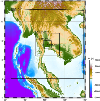
Fig. 1. Topography of computational domains for simulating solar irradiance with the meteorological model WRF. Observation site, NECTEC, is located at the center of Domain 3.
Download figure:
Standard image High-resolution image2.3. Computational conditions
The computational settings of weather simulation with WRF are summarized in Table I. The final analysis data of the NCEP operational Global Forecast System (GFS) 0.25-degree grids (horizontal resolution 0.25° × 0.25°, three-hourly interval) 31) are used as the initial and boundary conditions and data assimilation for model simulation. The NCEP data are re-analyzed as part of the forecasted data, NCEP GFS-0.25, which are used by the authors to forecast the solar irradiance in Thailand. 12)
Table I. Computational conditions of the meteorological model WRF for forecasting solar irradiance in Thailand.
| Period | 2017-01-01_00:00 UTC ∼ 2018-01-01_00:00 UTC |
| Input data | NCEP FNL-0.25 (three-hourly, 0.25° × 0.25°) |
| Nesting | 2-way nesting |
| Domain (horizontal resolution, number of grids) | Domain 1 (18 km, 100 × 100 grids) |
| Domain 2 (6 km, 100 × 100 grids) | |
| Domain 3 (2 km, 100 × 100 grids) | |
| Vertical layer | 50 levels (from surface to 100 hPa) |
| FDDA option | Enable (Domain 1 only) |
The computed global horizontal irradiance at the target point is output every 10 min, and the accuracy of the simulation is evaluated by comparison with the observation data.
The target period of simulation is a whole year from January to December in 2019. Before simulation, spin-up computation was performed for one day.
2.4. Observation data
The global horizontal solar irradiance and meteorological parameters, e.g. wind speed and ambient temperature, are observed at NECTEC, which is in the center of Domain 3 in Fig. 1, for references of the simulation, as previously explained. The sampling interval of the observation is 1 min. Since the WRF output is a 10 min interval, 10 min average observational data is used in this study.
2.5. Sensitive analysis of parameterization options
First, we selected six primary physical parameterization options; PBL, surface layer, cumulus, shortwave radiation, longwave radiation and microphysics, which may affect the accuracy of weather simulation in the tropics. Then one-year WRF simulations were performed with different combinations of schemes of the options. Then, the accuracy of the simulations was evaluated with a statistical error index, and the optimal combination of schemes is found. However, the weather simulation is computationally expensive, and since there are numerous combinations of the options it is not feasible to compute all of them. Consequently, the most commonly used schemes are selected and tested for the sensitive analysis in this study.
There are several statistical error indices, e.g. correlation coefficient (Corr) and rms error (RMSE). In this study, we employ the Corr of the irradiance as an evaluation index of the simulation error to the observation because it can assess the accuracy of the short-period variations, less than one day, of the irradiance.
The Corr and RMSE are defined as follows:


where xi
and yi
are simulated and observed diurnal irradiances,  and
and  are averages of x and y, respectively, and n is the number of data xi
or yi
.
are averages of x and y, respectively, and n is the number of data xi
or yi
.
If the Corr is large, the simulation error on the RMSE may be caused by the tendencies of WRF itself, e.g. overestimation, and it may be improved with a post-processing of WRF simulation. We will adopt this approach in future work.
3. Computational results and discussion
3.1. Seeking optimal combination of schemes of physical parameterization options
We seek the optimal combination of schemes of physical parameterization options in a similar way to Arasa et al. 15) A total of 20 simulations with different schemes have been performed progressively. The combinations of schemes for the simulations are listed in Table II. First, we performed WRF computation with the initial setup of schemes (Experimental name: INI). They are MYNN2, 32,33) Eta sim, 34–37) KF, 38) Dudhia, 39) RRTMG 40) and Thomson 41) for the options PBL, surface layer, cumulus, shortwave radiation, longwave radiation and microphysics, respectively. Next, the microphysics option changed from Thomson to WSM3, 42) WSM6 43) and SBU-Lin 44) in order, and the best scheme for the microphysics option was determined from the Corr of the solar irradiance between WRF simulation and observation. Then, the microphysics option was fixed with the best scheme, and the longwave radiation option was changed from RRTMG to Goddard, 45,46) RRTM 47) and FLG. 48,49) Similar processes were performed for cumulus with BMJ, 35) Grell 3D 50,51) and New SAS, 52) and for PBL with YSU, 53) MYJ, 35) QNSE, 54) ACM2, 55) MYNN3, 32,33) UW 56) and GBM. 57) The surface layer was changed by following PBL, because its selection is briefly dependent on the PBL. Table III shows the Corrs of each experimental case, and Table IV shows the optimal combination of schemes of the parameterization options selected with the sensitive analysis. The experimental case PBL1 has the highest Corr, as in Table III, and it is the optimal one. The RMSE for each case is also printed as a reference. For the experimental cases LWR3, SWR2 and PBL3 the numerical simulations were not completed due to instability of the model, and neither Corr nor RMSE was evaluated, as shown in the table. Therefore, their applicability could not be determined. The instability may occur at sudden change in the weather, and neither the time-step nor the grid resolution is responsible for the change.
Table II. Experimental cases of physical parameterization options.
| Experiment | PBL | Surface layer | Cumulus | Shortwave radiation | Longwave radiation | Microphysics |
|---|---|---|---|---|---|---|
| INI | MYNN2 | Eta sim | KF | Dudhia | RRTMG | Thompson |
| MPH1 | MYNN2 | Eta sim | KF | Dudhia | RRTMG | WSM3 |
| MPH2 | MYNN2 | Eta sim | KF | Dudhia | RRTMG | WSM6 |
| MPH3 | MYNN2 | Eta sim | KF | Dudhia | RRTMG | SBU-Lin |
| LWR1 | MYNN2 | Eta sim | KF | Dudhia | Goddard | Best microphysics |
| LWR2 | MYNN2 | Eta sim | KF | Dudhia | RRTM | Best microphysics |
| LWR3 | MYNN2 | Eta sim | KF | Dudhia | FLG | Best microphysics |
| SWR1 | MYNN2 | Eta sim | KF | RRTMG | Best longwave | Best microphysics |
| SWR2 | MYNN2 | Eta sim | KF | FLG | Best longwave | Best microphysics |
| CMS1 | MYNN2 | Eta sim | BMJ | Best shortwave | Best longwave | Best microphysics |
| CMS2 | MYNN2 | Eta sim | Grell 3D | Best shortwave | Best longwave | Best microphysics |
| CMS3 | MYNN2 | Eta sim | New SAS | Best shortwave | Best longwave | Best microphysics |
| PBL1 | YSU | MM5 | Best cumulus | Best shortwave | Best longwave | Best microphysics |
| PBL2 | MYJ | Eta sim | Best cumulus | Best shortwave | Best longwave | Best microphysics |
| PBL3 | QNSE | QNSE | Best cumulus | Best shortwave | Best longwave | Best microphysics |
| PBL4 | ACM2 | MM5 | Best cumulus | Best shortwave | Best longwave | Best microphysics |
| PBL5 | MYNN2 | MYNN | Best cumulus | Best shortwave | Best longwave | Best microphysics |
| PBL6 | MYNN3 | MYNN | Best cumulus | Best shortwave | Best longwave | Best microphysics |
| PBL7 | UW | MM5 | Best cumulus | Best shortwave | Best longwave | Best microphysics |
| PBL8 | GBM | MM5 | Best cumulus | Best shortwave | Best longwave | Best microphysics |
Table III. Statistical error indices of experimental cases (Experiment INI is with the initial setup of options and the experiment with the optimal schemes is PBL1).
| Experiment | Corr | RMSE (W m−2) |
|---|---|---|
| INI | 0.7733 | 241.5 |
| MPH1 | 0.7750 | 239.6 |
| MPH2 | 0.7774 | 238.4 |
| MPH3 | 0.7748 | 226.3 |
| LWR1 | 0.8021 | 214.4 |
| LWR2 | 0.7801 | 214.7 |
| LWR3 | (Incomplete computation) | |
| SWR1 | 0.7880 | 209.1 |
| SWR2 | (Incomplete computation) | |
| CMS1 | 0.7985 | 216.6 |
| CMS2 | 0.7846 | 220.6 |
| CMS3 | 0.7991 | 221.5 |
| PBL1 | 0.8143 | 204.7 |
| PBL2 | 0.8022 | 213.9 |
| PBL3 | (Incomplete computation) | |
| PBL4 | 0.7453 | 228.2 |
| PBL5 | 0.8047 | 212.8 |
| PBL6 | 0.8098 | 211.2 |
| PBL7 | 0.8077 | 207.7 |
| PBL8 | 0.8033 | 212.6 |
Table IV. Change in statistical error indices due to selecting optimal schemes of parameterization options.
| Parameterization option | Corr | RMSE (W m−2) |
|---|---|---|
| Microphysics | 0.0048 | 15.2 |
| Longwave radiation | 0.0274 | 11.9 |
| Shortwave radiation | 0.0142 | 5.3 |
| Cumulus | 0.0175 | 7.1 |
| Surface layer and PBL | 0.0690 | 23.6 |
The schemes of the parameterization options selected are summarized. SBU-Lin for microphysics considers quick growth of ice crystals (riming). Goddard for longwave radiation focuses on the solar irradiance transmission. Dudhia for shortwave radiation was developed under the winter conditions of the South China Sea. KF for cumulus parameterization contains the large-scale convection process with time scale of downdrafts or convective available potential energy. MM5 for the surface layer is the scheme developed for the former weather model MM5 (Fifth-Generation Penn State/NCAR Mesoscale Model). 58–60) YSU for PBL represents convection reduction with high accuracy.
Brief explanations of the other schemes listed in Table II are in the Appendix
3.2. Improvement of simulated solar irradiance
The Corrs with the initial setup (Experiment INI) and the optimal schemes (Experiment PBL1) are 0.773 and 0.814, respectively, as in Table III. The Corr increases 0.041 by the optimization. The evaluation index for the optimization is Corr, but the RMSE is also improved from 241.5 to 204.7 W m−2 by introducing the optimal ones.
Figure 2 shows 30-day moving averages of statistical error indices, Corr and RMSE of the solar irradiance simulations of all experimental cases. Winter in Thailand, from November to the next mid-March, has dry weather and is usually fine. As the Corr under the initial setting (INI) in Fig. 2(a), the WRF can simulate solar irradiance with high accuracy in this season. On the other hand, in summer, from mid-March to mid-May, there are cloudy and rainy days and the solar irradiance changes due to shading by clouds. Simulation of the irradiance with WRF becomes difficult and its accuracy reduces, as shown by the Corr in the figure. In the rainy season, from mid-May to October, the weather is even worse for the solar irradiance simulation, and its Corr drops to 0.7.
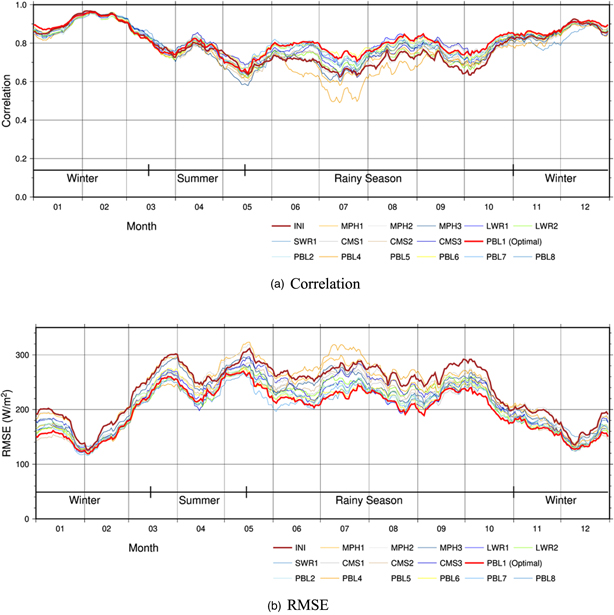
Fig. 2. 30-day moving averages of statistical error indices (Corr and RMSE) of all experimental cases. Cases of the initial, INI, and optimal combinations of parameterization options, PBL1, are plotted with thick lines.
Download figure:
Standard image High-resolution imageThe Corr of the case with the optimal combination is not at its highest in all months, as shown in Fig. 2(a), but it is the highest over the year, as listed in Table III. The Corr in the rainy season improved compared to the one in summer, by about 0.8, by introducing the optimal combination of schemes, as shown in the figure. However, there is very little improvement in simulation accuracy in summer, as shown in the figure. The application of the optimal schemes does not contribute to the improvement in this season. Since sufficient accuracy had already been obtained in winter with the initial setup of the schemes, the improvement in accuracy with the optimal schemes was limited.
The Corrs of monthly simulations improved throughout the year by introducing the optimal combination of schemes, as shown in Fig. 2(a). Only in February, does the Corr of the optimal schemes deteriorate, but only slightly.
The monthly RMSEs in Fig. 2(b) show the same trend as the Corrs in Fig. 2(a); higher accuracy in winter than in the other seasons. The RMSEs are reduced throughout the year by introducing the optimal schemes. The optimization of the parameterization options is for improving Corr only, but as a result, the RMSE is also improved by the optimization. The improving of monthly Corrs by the optimal schemes is limited in winter and summer, but the RMSEs are reduced by the optimal schemes in all the seasons.
The correlation maps of observed and simulated solar irradiance in April are plotted in Fig. 3. April is in summer, and the irradiance fluctuates strongly due to cloud shading. The fluctuation makes forecasting or representation of the irradiance difficult in this season. The red lines in the graphs are regression lines. Their slopes with (a) the initial and (b) the optimal combinations of schemes are 1.131 and 1.048, respectively. As can be seen in Fig. 3(a), WRF overestimates the irradiance, and the slope of the regression line is more than unity. The overestimation is canceled by introducing the optimal schemes, as shown in Fig. 3(b). Similar trends to in April are observed in other months. In April, the Corr is not improved by introducing the optimal schemes, but the RMSE is improved, as shown in Fig. 2. The reason is the cancellation of WRF overestimation, as shown in Fig. 3.
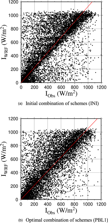
Fig. 3. Correlation maps of observed and simulated solar irradiance in April 2017. Red lines are regression ones. Their slopes are (a) 1.131 and (b) 1.048.
Download figure:
Standard image High-resolution imageAs shown in Figs. 2 and 3, the introduction of the optimal combination of scheme is effective throughout the year, especially in rainy season, from mid-May to October.
Figures 4 and 5 show the simulated and observed solar irradiance from July 26–28, 2017 during the rainy season. The weather was unstable and the solar irradiance fluctuated due to cloud shading, as shown in the figures. During the rainy season the solar irradiance varies quickly due to the clouds. Therefore, forecasting or representation of the weather and the irradiance with WRF is difficult, as shown in the figures.

Fig. 4. Simulated and observed daily solar irradiance with all combinations of parameterized options listed in Table II.
Download figure:
Standard image High-resolution image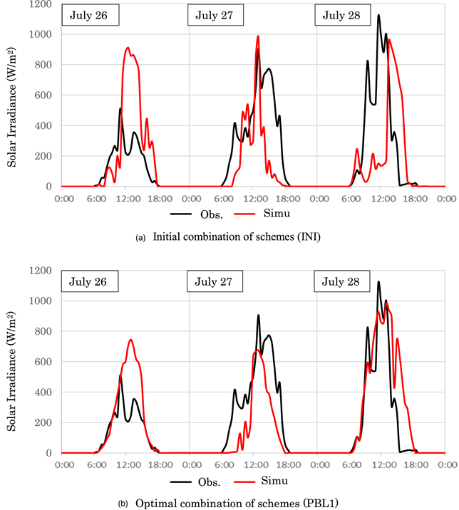
Fig. 5. Simulated and observed daily solar irradiance with (a) initial and (b) optimal combinations of parameterized options.
Download figure:
Standard image High-resolution image
Figure 4 shows all the simulated solar irradiance with the combination of schemes listed in Table II. There are large variations between the experimental cases, and this indicates the importance of setting up the parameterization options. In this figure, the simulated irradiance is larger than the observation in most of the experimental cases on 26 July. On the other hand, the irradiance is underestimated in most of the cases on 27 July. It can also be seen in the figure that the short-period variations do not correlate well with the simulation in this period.
Figure 5 shows the solar irradiance simulated with (a) the initial combination of schemes and (b) the optimal one. By introducing the optimal schemes, the simulated irradiance is reduced and comes near to the observation on 26 July. After a few days, the irradiance simulated with the optimal schemes is larger than the one with the initial conditions, and the simulation accuracy is improved with the optimal ones. The simulated short-period fluctuations of the irradiance are also improved and match the observation by introducing the optimal combination of schemes of the physical parameterization options.
In this study, the optimal combination of schemes is found, and its introduction improves the simulation accuracy. However, there is room for improvement in the simulation accuracy, as shown in Fig. 4(b). A complete simulation with an NWP model is not feasible due to its imperfections. A method to improve accuracy is to introduce a post-processing for NWP simulation, e.g. Zhang and Zou. 61) Probabilistic forecasting, e.g. Liu et al. 62) may also be useful for weather and solar irradiance forecasting.
3.3. Contributions of schemes of physical parameterization options to simulation accuracy
Table IV shows the changes in Corrs depending on each change in parameterization option. The changes in RMSE are also printed as a reference. We had expected that the accuracy of solar irradiance would be greatly affected by shortwave radiation processes and cumulus parameterization because of its large fluctuation due to cloud cover. However, Table IV shows that the surface layer and PBL display the largest change for improving Corr. This indicates that the surface layer and PBL have the greatest influence on the simulation accuracy of the solar irradiance. The surface layer process is a physical process that describes the exchange of heat and water vapor between the ground surface and the atmosphere, and the PBL process is a physical process that describes turbulent mixing in PBL. In considering the factors that significantly affect the accuracy of solar irradiance computations, the development of convective clouds, e.g. cumulus, should be discussed. The conditions for the development of convective clouds require unstable atmosphere and upwelling in the lower layers that triggers convection, or upwelling that lifts the entire air layer with unstable convection. Some lower-level upwelling is convection caused by heating of the ground surface. This is caused by heating of the ground surface by solar irradiance, which warms the atmosphere from the bottom. This convection occurs within the PBL, which includes the ground layer. Consequently, the surface layer and PBL are highly relevant to the prediction of convective clouds in the tropics.
3.4. Comparison of optimal combination of schemes with previous studies
The optimal schemes selected in the previous studies and the results in this study are compared here. Table V shows the list of the optimal schemes obtained in this study and by Zempila et al. 28) and Verbois et al. 29) Meteorological data sets for initial and boundary conditions are also indicated in the table. The schemes used in Arasa et al. 15) and Aryaputera et al. 11) are also listed as a reference because Arasa et al. 15) also optimized schemes, not for solar irradiance, but for wind. The target area of Aryaputera et al. 11) is Singapore, near Thailand, but their work did not include optimization of the options, and all the schemes are fixed from the beginning. The six parameterization options that are used in this study are listed in the table. The only target option for the optimization in both Zempila et al. 28) and Verbois et al. 29) is shortwave radiation. Other schemes were fixed from the beginning. They are indicated with parentheses in the table. The target area of Verbois et al. 29) is Singapore and it is near our target area, Thailand. The distance between them is about 1,500 km. However, the two points are about 13° apart in latitude, with Singapore at 1.4° and Thailand at 14.1°, in terms of north-south relationship.
Table V. Comparison of optimal combination of schemes and meteorological data sets for initial and boundary conditions of this study and in the previous studies, Zempila et al. 28) Verbois et al. 29) Arasa et al. 15) and Aryaputera et al. 11) (Parentheses indicate the schemes fixed from the beginning. The study by Aryaputera et al. 11) does not include optimization of parameterization options).
| This study | Zempila et al. 28) | Verbois et al. 29) | Arasa et al. 15) | Aryaputera et al. 11) | ||
|---|---|---|---|---|---|---|
| Country | Thailand | Greece | Singapore | South Spain | Singapore | |
| Climate | Tropics | Mediterranean | Tropics | Mediterranean | Tropics | |
| Objective variable | Solar irradiance | Solar irradiance | Solar irradiance | wind | — | |
| Number of target options | 6 | 1 | 1 | 6 | — | |
| Parameterization options | Microphysics | SBU-Lin | (Thompson) | (Thompson) | SBU-Lin | (WSM6) |
| Longwave radiation | Goddard | (RRTMG) | (RRTMG) | RRTMG | (RRTM) | |
| Shortwave radiation | Dudhia | Dudhia | Dudhia | Dudhia | (Dudhia) | |
| Cumulus | KF | (Grell-Devenyi) | (KF) | KF | (Grell-Freitas) | |
| Surface layer | MM5 | (unknown) | (unknown) | MM5 | (MM5) | |
| PBL | YSU | (MYJ) | (MYNN2) | YSU | (YSU) | |
| Meteorological data set for initial and boundary conditions | Re-analysis data of GFS with 0.25-degree | Re-analysis data of GFS with 1.0-degree | GFS with 0.5-degree | NCEP/NCAR CFS re-analysis v2 with 0.5-degree | GFS with 0.5-degree | |
As shown in the table, the optimal scheme for the shortwave radiation option in both previous studies, Zempila et al. 28) and Verbois et al. 29) is Dudhia, which is the same as in this study. Arasa et al. 15) also selected Dudhia as the optimal scheme for shortwave radiation, even though the target areas and climates are different. The scheme is relatively old, simple and has a low computational cost compared to the others. These results suggest that newer, more sophisticated, higher-order schemes are not necessarily better, but the combination with other parameterization options is more important.
When our optimal schemes are compared with the results of Arasa et al. 15) in Table V, only the longwave radiation option is different, Goddard and RRTMG, respectively. Our and their target areas are Thailand and southern Spain, and their climates are tropical and Mediterranean. In the process to evaluate the transmission of the irradiance, Goddard simply evaluates the absorption coefficient with the reference pressure and temperature. On the other hand, RRTM and its advanced scheme, RRTMG, evaluate the absorption coefficient along the optical path of the irradiance under various atmospheric conditions by paying a high computational cost. Therefore, for the atmosphere with high non-homogeneity, RRTMG evaluates the irradiance with higher accuracy than Goddard. This is the physical reason for the difference between the optimal longwave scheme in our study and that of Arasa et al. 15) The difference in climates may be the cause of the difference in the longwave radiation option.
In previous studies, Zempila et al. 28) and Verbois et al., 29) some parameterization options are fixed from the beginning, and they are different to the ones that are derived as the optimal ones in this study, as shown in Table V. The simulation accuracy with different schemes in the table are compared here. As discussed in the previous section, PBL and surface layer options make a large contribution to the simulation accuracy. The accuracy of the schemes for the options are listed in Table VI. The schemes for the surface layer option in both Zempila et al. 28) and Verbois et al. 29) are not known. Thus, we compare the schemes of PBL options only in the table. The Corr and RMSE for each scheme are listed in the table. The Corr of the experiment with the YSU scheme is 0.01 higher than the others, and its RMSE is also smaller.
Table VI. Statistical error indices of solar irradiance forecasting with optimal schemes of the PBL option in this study and the previous studies of Zempila et al. 28) and Verbois et al. 29)
| This study | Zempila et al. 28) | Verbois et al. 29) | ||
|---|---|---|---|---|
| Parameterization options | PBL | YSU | MYJ | MYNN2 |
| Surface layer | MM5 | (Eta sim) | (MYNN) | |
| Experiment (in this study) | PBL1 | PBL2 | PBL5 | |
| Error indices (in this study) | Corr | 0.814 | 0.802 | 0.805 |
| RMSE (W m−2) | 204.7 | 213.9 | 212.8 |
As shown in Table V, the shortwave radiation option of the optimal combination in this study is Dudhia, which is the same as the optimal one in the previous studies. From this table, one can see the commonality of each optimal combination or setting for the parameterization options for forecasting solar irradiance or for forecasting in the tropics. This result will be helpful for other researchers to set up NWPs under similar conditions.
4. Conclusion
The short-period forecasting system of solar irradiance in Thailand has been developed and operated using the numerical meteorological model, WRF, to predict the generation of PV systems. In this study, the system is improved by the optimization of schemes of physical parameterization options in WRF. The target country, Thailand, is in the tropics, and the weather is complicated due to the vertical behavior of clouds, e.g. cumulus and cumulonimbus, and sudden changes, e.g. squalls. The complicated weather makes forecasting difficult for WRF. It is necessary to seek and find the optimal schemes that are required to increase the accuracy of forecasting in the area. The six primary physical parameterization options, PBL, surface layer, cumulus, shortwave radiation, longwave radiation and microphysics are selected as ones that may affect the accuracy of weather simulation in the tropics. The sensitive analysis of the options is performed by changing schemes of the options in order, and the optimal combination of the schemes is found. They are SBU-Lin, Goddard, Dudhia, KF, MM5 and YSU for microphysics, longwave radiation, shortwave radiation, cumulus, surface layer and PBL, respectively. The Corr of solar irradiance between the simulation and observation is improved from 0.773 to 0.814 by introducing the optimal schemes from the initial computational conditions. This optimization improved the Corrs mainly during the rainy season, from mid-May to October, but improved the RMSE throughout the year. The WRF overestimated the solar irradiance with the initial setup of schemes, and the overestimation is canceled by the optimization of options. The RMSE is improved by the cancellation. The optimized simulation represents the intensity of the irradiance, which compares well with the observation. The simulated irradiance also effectively traces the short-period fluctuations in the observed one. The contributions of the parameterization options to the solar irradiance simulation are also discussed, and it is found that the surface layer and PBL have a significant impact on the simulation.
Appendix
Table A·I. The schemes used as the physical parameterization options in this study are summarized.
| Physical parameterization option | Scheme | Summary |
|---|---|---|
| Microphysics | Thomson graupel 41) | Processes for ice crystals, snow and hail in high-resolution simulations are considered. |
| Particle density of precipitation is evaluated. | ||
| WSM3 42) | Processes for ice crystals and snow in mesoscale simulations are considered. | |
| WSM6 43) | Processes for ice crystals, snow and hail in high-resolution simulations are considered. | |
| SBU-Lin 44) | Quick growth of ice crystals (riming) is considered. | |
| Computational processes are reduced by gathering hail and snow into one parameter, and therefore the computational time is also reduced. | ||
| Longwave radiation | RRTMG 40) | An improved version of RRTM. |
| The radiation under the condition in which the clouds overlap can be evaluated as a result of the improvement. | ||
| Goddard 45,46) | Focuses on transmission of the solar irradiance. | |
| RRTM 47) | Absorption of the radiation due to vapor, ozone, hydro-carbon, methane, nitrous oxide, oxygen, nitrogen and halocarbons are taken into account. | |
| FLG 48,49) | Radiation process effected by cirrus is considered. | |
| Shortwave radiation | Dudhia 39) | Developed for the simulation of the convection over the South China Sea in winter. |
| RRTMG | (Same as RRTMG of longwave radiation) | |
| FLG | (Same as FLG of longwave radiation) | |
| Cumulus | KF 38) | Contains the large-scale convection process with time scale of downdrafts or convective available potential energy (CAPE). |
| BMJ 35) | Suitable for representing tropical cyclones and heavy rain. | |
| Grill 3D 50,51) | Introduces the ensemble forecasting method and data assimilation technique. | |
| New SAS 52) | Precipitation in North America and tracks of hurricanes in the Pacific Ocean are forecast with high accuracy with this scheme. | |
| Surface layer | Eta sim 34–37) | Considers mixing process of turbulent atmosphere. |
| Wind speed distributions under various temperature conditions are generalized. | ||
| MM5 | Scheme developed for the former weather model MM5 (Fifth-Generation Penn State/NCAR Mesoscale Model). 58–60) | |
| QNSE | Specialized scheme for QNSE of the PBL option. | |
| MYNN | Specialized scheme for MYNN2 and MYNN3 of the PBL option. | |
| Planetary boundary layer (PBL) | MYNN2 32,33) | Kinematic turbulent energy in sub-grid is evaluated. |
| Computational cost is low. | ||
| YSU 53) | Can represent convection reduction with high accuracy. | |
| MYJ 35) | 1D kinematic turbulent energy scheme. | |
| QNSE 54) | Introduces new theory for stable stratification. | |
| ACM2 55) | Improves the representation of vertical temperature distributions by taking eddy diffusion into account. | |
| MYNN3 32,33) | Kinematic turbulent energy in sub-grid is evaluated. | |
| Represents the upper layer of the PBL with high accuracy. | ||
| UW 56) | Kinematic convection energy scheme based on the CAM model. 63) | |
| GBM 57) | Considers the stratocumulus boundary layer for computations with low vertical resolution. |