
Abstract
In sound wave propagation in the sea, it is important to evaluate the characteristics of sound reflection from the sea surface. The amplitude and phase of reflected sound waves fluctuate because of the changing sea surface with waves. In this study, using the finite difference time domain method and experiments in a water tank, we evaluated the variability characteristics of reflected sound waves on the sea surface generated by the Bretschneider-Mitsuyasu spectrum observed on the deep offshore coast of Japan. We introduced the concept of effective roughness of the sea surface and evaluated the variability characteristics of reflected sound waves on the sea surface. We confirmed the Rice distribution could express the amplitude variability, and the energy ratio γ is determined by the Rayleigh roughness parameter  defined by the effective roughness
Export citation and abstract BibTeX RIS
1. Introduction
In ocean development of resources and observations, it is indispensable to utilize underwater acoustic technology using sound waves propagating in seawater. When using underwater acoustic devices, we often evaluate the effect of sound reflection on the sea surface.
When sea surface waves are sufficiently calm, the assumption of specular reflections of the sound waves is valid for estimating acoustic propagation characteristics. On the other hand, the actual surface waves change randomly with time because of wind and gravity, and consequently, the amplitude and phase of reflected sound waves also fluctuate randomly. Especially when using sound waves in shallow sea environments, sound waves are strongly affected by the reflection of the sound waves on the seabed and sea surface. Therefore, it is important to clarify the characteristics of sea surface reflected waves that cause fluctuations in acoustic signals.
In recent years, many studies have been conducted on acoustic communication technology that enables wireless information transmission underwater. In the field of acoustic communication, the multipath wave and Doppler effect caused by sound wave propagation in the sea are obstacles to realizing robust and high-rate acoustic communication. 1–9) The use of acoustic communication is increasing not only in deep-sea areas but also in shallow water areas such as harbors and coastal regions. 4) In order to improve communication performance in shallow water environments, it is necessary to clarify the variability characteristics of sea surface reflected waves quantitatively. In this paper, we try to evaluate the variability characteristics of sound reflection on the sea surface, which is the major cause of fluctuations in multipath signals.
Several studies have reported the characteristics of reflected sound waves on the sea surface.
10–16) With the wave height increasing, the amplitude probability density function (PDF) of reflected sound waves can be expressed by the Rice distribution, which changes from the Gaussian distribution to the Rayleigh distribution.
17) In Ref. 17, the amplitude and phase variability characteristics were studied using experiments in a water tank with waves. Their study has demonstrated that  (
( wavenumber,
  root-mean-square (rms) of water level,
  incident angle) and energy ratio γ of the Rice distribution are in a fixed relationship in the evaluation of the amplitude variability. However, this conclusion applies only to the assumption that the sea surface is a sufficiently random rough surface. Therefore, the variability characteristics of reflected sound waves on the sea surface with a large surface wavelength and relatively smooth surface have not been clarified.
In our study, we evaluate the variability characteristics of reflected sound waves on the sea surface based on the Bretschneider-Mitsuyasu spectrum
18,19) observed on the deep offshore coast of Japan. The variability characteristics are investigated quantitatively by acoustic FDTD simulation
20,21) and the water tank test using hydraulic plungers.
22) We have already reported the effect of sea surface wavelength  on the variability characteristics of reflected sound waves on the sea surface. When the surface wavelength
  is small, and the sea surface can be regarded as a sufficiently random rough surface, it has been shown that the Rayleigh roughness parameter
  uniquely determines the energy ratio γ for amplitude variability. In addition, the standard deviation of phase
  for phase variability is determined by
  regardless of surface wavelength
  23) In Ref. 24, we investigated the effect of sea surface wavelength on the variability characteristics of reflected sound waves on the sea surface. However, quantitative characteristics of amplitude fluctuation have not yet been clarified.
In this paper, we define the effective roughness of the sea surface, which is determined by the surface wavelength and the distance between the sound source, receiver, and sea surface. Then, we evaluate the variability characteristics of reflected sound waves using effective roughness. Some results of evaluating the amplitude and phase variabilities using the new Rayleigh roughness parameter  with the effective roughness
  have already been reported as preliminary studies.
25) In this paper, we present a detailed explanation of the effective roughness of the sea surface and report the verification results of the validity of the effective roughness of the sea surface by the water tank test.
have already been reported as preliminary studies.
25) In this paper, we present a detailed explanation of the effective roughness of the sea surface and report the verification results of the validity of the effective roughness of the sea surface by the water tank test.
2. Methods
2.1. Acoustic simulation with the FDTD method
We use the 2D-FDTD simulation model shown in Fig. 1 to evaluate the variability characteristics of reflected sound waves. The analytic area is discretized by the staggered grid. The sound pressure and particle velocity on the grid point are calculated using the central difference scheme. In the FDTD simulation, the Gaussian pulse is transmitted from the sound source, and the surface boundary with zero pressure is generated by Eq. (1). Other boundaries are set perfectly matched layer (PML) to absorb sound waves. 26) Table I shows the basic parameters for the 2D-FDTD simulation model.

Fig. 1. (Color online) Underwater sound wave propagation model for 2D-FDTD method.
Download figure:
Standard image High-resolution imageTable I. Basic parameters for the 2D-FDTD simulation model.
| Parameters | Values |
|---|---|
| Sound source | Gaussian pulse |
| Analysis area | Width: 7 m, Depth: 3 m |
Density: 
| 1000 kg m−3 |
Sound speed: 
| 1475 m s−1 |
| Surface boundary condition | Sound pressure is zero |
| Side and bottom boundary condition | PML |
| Spatial step | 5 mm |
| Timestep | 1.7 us |
Surface wavelength: 
| 0.32–5.08 m |
rms of surface water level: 
| 4.12–37.1 mm |
In strictly, the reflected sound waves on the sea surface are affected by the Doppler effect because the sea surface fluctuates constantly. However, the fluctuating velocity of the sea surface is on the order of several seconds and is extremely small compared to the speed of sound in seawater (about 1500 m s−1). Therefore, in the calculation of the FDTD, the sea surface is treated as a stationary boundary with no temporal variation. Since this study aims to evaluate the sea surface reflection characteristics, which is the main factor of the multipath effect, there is no problem in treating the sea surface as a stationary boundary.
2.2. Sea surface waves following the Bretschneider-Mitsuyasu spectrum
Sea surface waves are represented by the superposition of regular waves with different surface wavelengths. In addition, sea surface waves are classified into dispersible waves having different phase velocities depending on the surface wavelength. The Bretschneider-Mitsuyasu spectrum shown in Eq. (1) is well known to give a good approximation of the sea surface spectrum that is observed on the deep offshore coast of Japan. In order to simulate sea surface waves, we used a single summation method 27,28) shown in Eq. (2) based on the Bretschneider-Mitsuyasu spectrum.


Here,  is the water level.

 and
and  represent the amplitude, the wavenumber, the frequency, and the initial phase.
  is the sampling number in the frequency domain.
  is the ocean wave spectrum,
  is the significant wave height, and
  is the significant wave period. In the calculation of
  shown in Eq. (1),
  (
( 9.8
9.8  ) and
) and  is randomly given in the range of 0–
 rad.
rad.
In the simulation using the FDTD method, the water level  at a certain time is set as the surface boundary. In order to evaluate the statistical properties of fluctuation of reflected sound waves, we generate a total of 250 surface boundaries observed every 0.3 s with the same
  and
and  conditions.
In this study, the wave height and wavelength of the sea surface are adjusted by controlling  and
and  in Eq. (1). In statistically evaluating the variability characteristics of reflected sound waves, the effective value of water level
  as overall sea roughness and the wavelength of the sea surface
  are defined as Eqs. (4) and (5), respectively.


Here, Eq. (4) is the Rayleigh roughness parameter  and is calculated from the water level directly above the sound source on the sea surface used in the FDTD simulation. Equation (5) shows the relationship between the wavelength
  and the period
  of sea surface waves observed under the condition of deep water waves dominated by gravity waves. Since the Bretschneider-Mitsuyasu spectrum has a frequency bandwidth, the expected value of the period T of sea surface waves is calculated from the Eq. (1), and the average wavelength
  of sea surface waves is defined. In the previous paper, the relationship
  and
and  are derived based on statistical theory.
29–32)
are derived based on statistical theory.
29–32)
2.3. Evaluation method of amplitude and phase variability of reflected sound waves
In this study, the Gaussian pulse used as the sound source is treated as impulse responses with a limited frequency band in order to reduce the numerical dispersion of the FDTD method. The amplitude and phase of reflected sound waves are calculated by convolving arbitrary tone burst waves with impulse responses obtained by the FDTD simulation.
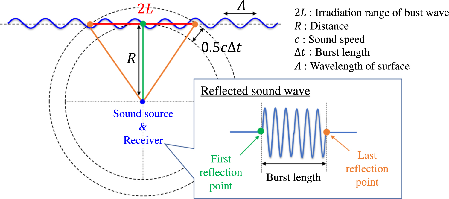
Figure 2 shows the irradiation range of burst waves on the sea surface that contributes to reflected sound waves. The reflection points on the sea surface directly above the sound source contribute to the rising part of burst waves. Then, the contribution from horizontally distant reflection points on the sea surface increase over time. The irradiation range of burst waves  can be described by Eq. (6). Here,
  is the distance from the sound source to the sea surface, sound speed
  and the tone burst wave length
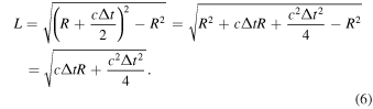
The longer the burst wavelength, the wider the irradiation range of sound waves on the sea surface that contributes to reflected sound waves. Since the distance attenuation becomes large and the angle of incidence of sound waves on the sea surface becomes shallow, the contribution from horizontally distant reflection points gradually decreases, and the amplitude and phase of reflected sound waves converge to a constant value. In this study, we evaluate the variability characteristics of reflected sound waves using the average amplitude  and phase
  in the 85%–95% section of the latter half of burst length contributed many reflection points.
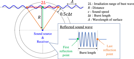
Fig. 2. (Color online) Irradiation range on the sea surface contributing to sound reflection. 23)
Download figure:
Standard image High-resolution image2.4. Evaluation of variability characteristics reflected sound waves by Rice distribution
When there is no wave on the sea surface, the reflected sound waves can be regarded as sound waves from the mirror image of the sound source. The reflected sound waves are coherent waves with no temporal fluctuation. As the wave height of the sea surface increases, reflection points randomly fluctuating on the sea surface increase. As a result, the coherent component of the reflected sound waves decreases, and the incoherent component gradually increases. The statistical properties of a signal in which coherent and incoherent components coexist can be represented by the Rice distribution. 33–36)
The PDF of amplitude variability in the Rice distribution can be shown as

where 
 and
and  are the probability density, the amplitude of the sound wave, and the modified Bessel function, respectively.
  is the energy ratio of the coherent and incoherent components, which is expressed by using an rms of sinewave
  and a rms of noise
  In the PDF of the amplitude variability of the Rice distribution, the Rayleigh distribution is obtained when
  and the Gaussian distribution when
  is large. Figure 3 shows the Rice distribution expressed using complex vectors. As shown in Fig. 3, the Rice distribution follows the normal distribution
  for the
  -axis and the normal distribution
  for the
  -axis in the complex plane. Assuming that the sea surface is a sufficiently random rough surface, previous studies
12–17) have shown that the variability characteristic of reflected sound waves can be described using the Rayleigh roughness parameter
-axis in the complex plane. Assuming that the sea surface is a sufficiently random rough surface, previous studies
12–17) have shown that the variability characteristic of reflected sound waves can be described using the Rayleigh roughness parameter  and the Rice distribution.

Fig. 3. (Color online) Vector representation of Rice distribution on the complex plane.
Download figure:
Standard image High-resolution imageHowever, we have reported that the variability characteristics of reflected sound waves change depending on the surface wavelength  even with the same Rayleigh roughness parameter
  24) In Ref. 24, we show that as
  becomes smaller, the variability characteristics displayed on the complex plane approach the Rice distribution shown in Fig. 3. Figure 4 shows the variability of reflected sound waves on the complex plane obtained under the condition that the Rayleigh roughness parameter
  is fixed and surface wavelength
  are changed in the FDTD simulation. Here, the data are normalized by the amplitude (
 ) and phase (
 ) observed under the condition that there is no wave on the sea surface. In addition, Fig. 4 expresses the effect of surface wavelength
  on variability characteristics using complex vectors. When
  is very large, and the sea surface can be regarded as a flat surface within the burst wave irradiation range, the sea surface acts as a specular reflection boundary. In this condition, only phase fluctuation according to the Rayleigh roughness parameter
  is observed without the amplitude fluctuation. This characteristic can be expressed by complex vectors in which the phase of coherent component
s
of reflected sound waves fluctuates according to
is observed without the amplitude fluctuation. This characteristic can be expressed by complex vectors in which the phase of coherent component
s
of reflected sound waves fluctuates according to  As
As  becomes smaller, irregularly fluctuating reflection points increase within the irradiation range of the burst wave on the sea surface. Therefore, the coherent component
s
of a reflected sound wave is gradually lost, and the incoherent component
n
increase. Under the condition that
becomes smaller, irregularly fluctuating reflection points increase within the irradiation range of the burst wave on the sea surface. Therefore, the coherent component
s
of a reflected sound wave is gradually lost, and the incoherent component
n
increase. Under the condition that  is small enough, the reflected sound waves from multiple randomly fluctuating reflection points interfere with each other with a phase difference according to
  As a result, the sea surface approaches a sufficiently random rough surface, and the variability characteristics of reflected sound waves converge to the Rice distribution described in previous studies.
12–17)
As a result, the sea surface approaches a sufficiently random rough surface, and the variability characteristics of reflected sound waves converge to the Rice distribution described in previous studies.
12–17)
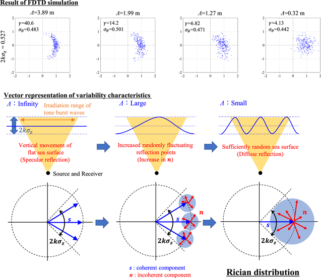
Fig. 4. (Color online) Result of FDTD simulation and vector representation of variability characteristics of reflected sound waves considering surface wavelength 
Download figure:
Standard image High-resolution image3. Results and discussion
3.1. Characteristics of reflected sound waves on a relatively smooth surface with a large 

In our previous study,
24) we could not quantitatively evaluate the variability characteristics of reflected sound waves on a relatively smooth surface with a large surface wavelength  In the FDTD simulation of sea surface wavelength, we found that the variability characteristics of reflected sound waves are different from the Rice distribution shown in Fig. 4 on a relatively smooth sea surface where
  is large. In this condition, it is considered that the geometrical similarity between the shape of the sea surface and sound wave directly contributes to the variability characteristics of reflected sound waves. For the variability characteristics of reflected sound waves to be the same on a relatively smooth surface, a geometric similarity relationship must be established between the shape of the sea surface and sound waves, as shown in Fig. 5 and Eq. (9). Here,
  is the distance between the sound source, receiver, and sea surface.
  is the wavelength of the sound wave.

 and
and  are normalized by the frequency of sound waves, such as
  and
and  respectively. The unit of
  and
and  is radians, which is the same as the Rayleigh roughness parameter

Fig. 5. (Color online) A geometric similarity relationship between the shape of the sea surface and sound waves.
Download figure:
Standard image High-resolution imageIn this section, we adjusted 
 and
and  so that
  and
and  are fixed, and we evaluated the effect of the geometrical similarity between the shape of the sea surface and sound waves on the variability characteristics of reflected sound waves. Table II shows the FDTD simulation conditions. Figure 6 shows the energy ratio
  of the Rice distribution for amplitude variability and the standard deviation
  for phase variability when the Rayleigh roughness parameter
  are changed under the fixed condition of
  and
and  In Fig. 6,
  and
and  are estimated by the maximum likelihood method using the amplitude and phase of reflected sound waves. When the sea surface is a sufficiently random rough surface,
  is uniquely determined by
  so that
  is displayed as
  in Fig. 6. Figure 6 shows that γ is determined by
  regardless of frequency,
  takes a different value depending on
  These results indicate that on a relatively smooth sea surface with large
 is larger than
  that is, the coherent component of reflected sound waves is large. Therefore, it is considered that the roughness of the sea surface, which is smaller than the overall sea roughness
  contributes to
  for amplitude variability of reflected sound waves. On the other hand,
  equals to
  regardless of
  which indicates
  contributes to
  for the phase variability.
Table II. FDTD simulation conditions evaluating the effect of geometrical similarity.
 [rad] [rad] |
 [rad] [rad] |
 [m] [m] |
 [Hz] [Hz] |
 [m] [m] |
|---|---|---|---|---|
| 8.95 | 53.25 | 0.32 | 6613 | 1.89 |
| 0.38 | 5465 | 2.29 | ||
| 0.42 | 5000 | 2.5 | ||
| 13.26 | 53.25 | 0.38 | 8099 | 1.54 |
| 0.42 | 7410 | 1.69 | ||
| 0.46 | 6806 | 1.84 | ||
| 0.50 | 6272 | 1.99 | ||
| 0.62 | 5000 | 2.5 | ||
| 20.72 | 53.25 | 0.62 | 7813 | 1.6 |
| 0.71 | 6806 | 1.84 | ||
| 0.81 | 5981 | 2.09 | ||
| 0.97 | 5000 | 2.5 | ||
| 27.07 | 53.25 | 0.81 | 7812 | 1.6 |
| 0.97 | 6531 | 1.91 | ||
| 1.09 | 5844 | 2.14 | ||
| 1.27 | 5000 | 2.5 | ||
| 42.29 | 53.25 | 1.27 | 7812 | 1.6 |
| 1.99 | 5000 | 2.5 | ||
| 60.90 | 53.25 | 1.99 | 7200 | 1.74 |
| 2.86 | 5000 | 2.5 | ||
| 82.89 | 53.25 | 2.86 | 6806 | 1.84 |
| 3.89 | 5000 | 2.5 | ||
| 108.26 | 53.25 | 2.86 | 8889 | 1.41 |
| 3.89 | 6531 | 1.91 | ||
| 5.08 | 5000 | 2.5 |
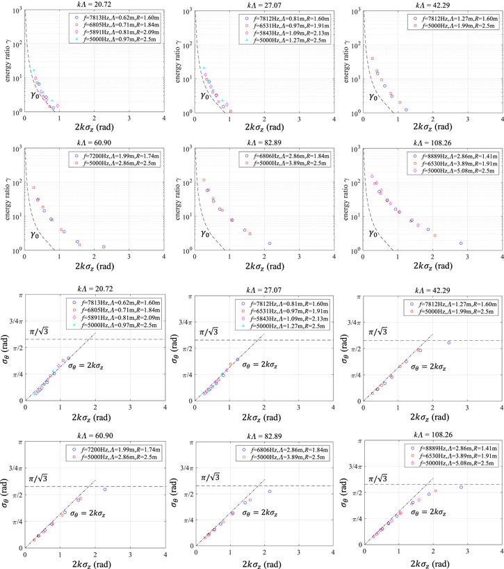
Fig. 6. (Color online) The energy ratio  and the standard deviation of phase
  depending on Rayleigh roughness parameter
  under the fixed condition of
  and
and 
Download figure:
Standard image High-resolution image3.2. Definition of the effective roughness of sea surface
From the results in the above section, it is considered that as the sea surface wavelength  increases, the sea surface roughness that contributes to reflected sound fluctuations becomes smaller than the overall sea surface roughness
We determine the range of the sea surface,  that contributes to the amplitude variability characteristics as shown in Fig. 7. The effective roughness,
  is defined as the roughness within the contribution range of this sea surface,
  The effective roughness is smaller than the roughness of the entire sea surface,
  when the sea surface wavelength,
  is large. The effective roughness increases as the sea surface wavelength,
  decreases. When
  is sufficiently small, and the sea surface approaches the random rough surface, the effective roughness becomes
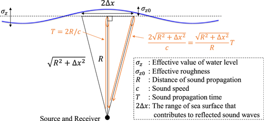
Fig. 7. (Color online) Definition of the effective roughness  the range of sea surface that contributes to reflected sound waves
  and sound propagation time
Download figure:
Standard image High-resolution imageThe energy ratio  which is a parameter of the Rice distribution that describes the amplitude variability characteristics of the reflected sound waves, can be determined by the new Rayleigh roughness parameter
  using the effective roughness of the sea surface
  as shown in Fig. 8. The Rayleigh roughness parameter,
  represents the phase difference between the reflection from the average water level and the reflection from crests and troughs of the entire sea surface waves. On a relatively smooth sea surface with a large
  the sea level range that contributes to the reflected sound waves is limited. The water level difference in this range is smaller than the overall water level difference, so the phase difference,
  is smaller than
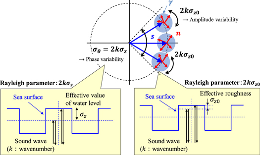
Fig. 8. (Color online) Definition of the new Rayleigh roughness parameter  for the amplitude variability and the Rayleigh roughness parameter
  for the phase variability.
25)
for the phase variability.
25)
Download figure:
Standard image High-resolution imageThe effective roughness of the sea surface  is estimated from the relationship between the energy ratio
  and the Rayleigh roughness parameter
  obtained in Fig. 6. We assume that the energy ratio
  obtained on a sufficiently random rough surface can be described uniformly by the Rayleigh roughness parameter
  expressed by the effective roughness
  of the sea surface. From the relationship between
  and
and  obtained by the FDTD simulation and the relationship between
  and
and  on the sufficiently random rough surface,
  is given by Eq. (10).

Figure 9 shows  obtained from the simulation results in Fig. 6. If
  is fixed,
  and
and  are in a proportional relationship, so
  is an almost constant value.
  approaches 1 when
  is sufficiently small and decreases as
  increases. The range of the sea surface that contributes to the amplitude variability
  is calculated from
  obtained by the FDTD simulation. From the shape of the sea surface used in the FDTD simulation, the spatial effective roughness
  is calculated for each
 can be calculated from
  corresponding
  obtained by the FDTD simulation. Since
  changes with
  we normalized
  using the sound wave propagation time shown in Fig. 7. As shown in Fig. 7, the propagation time from the sound source to the receiver is shown in
  where
where  is the speed of sound. Here,
  that contributes to the amplitude variability can be replaced with the range irradiated during the sound wave propagation time of
  Therefore, the propagation time that contributes to amplitude variability is expressed by Eq. (11) using
  Here, the coefficient of sound wave propagation time,
  is defined by Eq. (12). Table III shows the
  and
and  obtained by the FDTD simulation.


The coefficient of sound wave propagation time,  is almost the same in any
  There is a slight difference in
  due to the difference in
  but it is considered that the backscattering component from the reflection point horizontally away from the reflection point directly above the sound source has changed due to the difference in
  Under the simulation conditions of this paper, the average value of
  is calculated as
  = 1.0052. The relationship between
  and
and  is given by Eq. (13). Equation (13) shows that the sea surface range
  corresponding to about 1/5 of
  contributes to the amplitude variability. Equation (13) is estimated from the shape of the sea surface based on the Bretschneider-Mituyasu spectrum, and the relationship changes depending on the wave spectrum

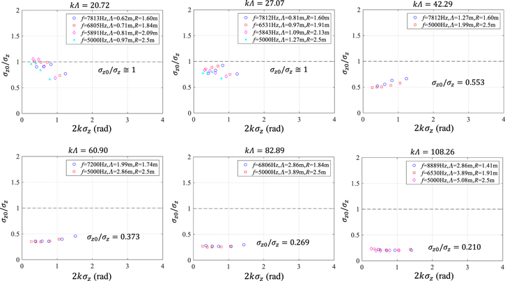
Fig. 9. (Color online) Calculation of the effective roughness  of the sea surface from the result of Fig. 7.
Download figure:
Standard image High-resolution imageTable III. Estimating the coefficient of sound propagation time  from the result of FDTD simulation in Fig. 6.
 [rad] [rad] |

|
 [m] [m] |
 [Hz] [Hz] |
 [m] [m] |
 [m] [m] |

|
|---|---|---|---|---|---|---|
| 42.29 | 0.553 | 1.27 | 7812 | 1.6 | 0.195 | 1.0074 |
| 1.99 | 5000 | 2.5 | 0.32 | 1.0082 | ||
| 60.90 | 0.373 | 1.99 | 7200 | 1.74 | 0.175 | 1.0051 |
| 2.86 | 5000 | 2.5 | 0.26 | 1.0054 | ||
| 82.89 | 0.269 | 2.86 | 6806 | 1.84 | 0.17 | 1.0043 |
| 3.89 | 5000 | 2.5 | 0.235 | 1.0044 | ||
| 108.26 | 0.210 | 2.86 | 8889 | 1.41 | 0.125 | 1.0039 |
| 3.89 | 6531 | 1.91 | 0.175 | 1.0042 | ||
| 5.08 | 5000 | 2.5 | 0.23 | 1.0042 |
3.3. Verification of the effective roughness of sea surface
In this section, we verified the effect of the effective roughness  on the variability characteristics of reflected sound waves. Table IV shows the test parameters for the FDTD simulation. In the simulation, the distance between the sound source, receiver, and sea surface
  is fixed at 2.5 m, and the sea surface range
  that contributes to the amplitude variability is calculated to be 0.51 m from Eq. (13). Figure 10 shows the relationship between the effective roughness
  and
and  under the condition of
  = 0.51 m obtained from the shape of the sea surface used in the FDTD simulation.
Table IV. Test parameters for FDTD simulation verifying the effective roughness of sea surface.
| Parameter | Value |
|---|---|
Frequency: 
| 2.5, 5, 7.5, 10 kHz |
Tone burst length: 
| 2.4 ms |
| Tone burst interval | 0.3 s |
| Number of data | 250 |
Distance: 
| 2.5 m |
Incident angle of sound:
| 0 deg |
Sound speed: 
| 1475 m s−1 |
Wavelength of sea surface wave: 
| 0.32–5.08 m |
rms of water level: 
| 4.12–37.1 mm |

Fig. 10. (Color online) Relationship between the effective roughness  and sea surface wavelength
Download figure:
Standard image High-resolution imageFigure 11 shows the variability characteristics of reflected sound waves obtained when the sea surface wavelength  and the frequency
  of the sound wave are changed. The energy ratio
  indicating the amplitude variability can be uniquely described by the new Rayleigh roughness parameter
  expressed by the effective roughness
  and the value converges to the energy ratio
  of the Rice distribution. The phase variability
  can be uniquely described by the Rayleigh roughness parameter
  expressed by the overall sea roughness
  This means that the long-term vertical movement of sea surface corresponding to
  appears as phase fluctuation. Figure 11 shows that the amplitude variability characteristic is determined by the local fluctuation in the shape of the sea surface roughness observed on a short time scale, and the phase variability characteristic is determined by the global fluctuation in the overall sea surface roughness observed on a long-time scale. Previous studies
12–17) have been limited to discussing the variability characteristics of reflected sound waves on a sufficiently random rough surface. We have clarified that the variability characteristics of reflected sound waves on a relatively smooth surface with a large surface wavelength
appears as phase fluctuation. Figure 11 shows that the amplitude variability characteristic is determined by the local fluctuation in the shape of the sea surface roughness observed on a short time scale, and the phase variability characteristic is determined by the global fluctuation in the overall sea surface roughness observed on a long-time scale. Previous studies
12–17) have been limited to discussing the variability characteristics of reflected sound waves on a sufficiently random rough surface. We have clarified that the variability characteristics of reflected sound waves on a relatively smooth surface with a large surface wavelength  can be expressed using effective roughness

Fig. 11. (Color online) The relationship between the energy ratio  and
and  for the amplitude variability and the relationship between the standard deviation of phase
  and
and  for the phase variability.
Download figure:
Standard image High-resolution image3.4. Water tank test
This section report the validity verification of the effective roughness of the sea surface by the water tank experiment. Figure 12 shows the configuration of acoustic devices in a water tank. We controlled the hydraulic drive plungers and generated surface waves according to Eq. (1) spectrum. Omnidirectional hydrophones were used for the sound source and the receiver. The size of a water tank is depth 5 m, width 10 m, and length 210 m. The transducer and hydrophone are set at a depth of 2 m. The sound source transmitted tone burst waves repeatedly from the function generator through a power amplifier, and the received signals were recorded using a data logger through a charge amplifier.
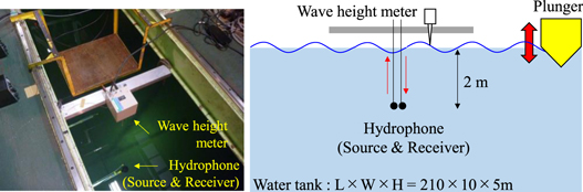
Fig. 12. (Color online) Configuration of the acoustic devices in water tank test.
Download figure:
Standard image High-resolution imageTable V shows the test parameters for the water tank test. The tone burst length was set to 1.0 msec to separate the reflected sound waves from the sea surface and the wall of the water tank. In order to suppress the effect of reverberation of the tank wall, the tone burst interval was set to a long cycle of 0.3 s. The effective value of water level  was calculated from the data of the wave height meter. Figure 13(a) shows a result of the measurement of water level obtained
  mm condition. From the expected value of wave period
  observed by the wave height meter and Eq. (5), the surface wavelength
  in the water tank test is calculated to be 4.1 m. In the water tank test, the surface wavelength
  was fixed, and we obtained the variability characteristics data when the water level was changed. Figure 13(b) shows the spectrum of the surface waves obtained in the water tank test.
Table V. Test parameters of water tank test.
| Parameter | Value |
|---|---|
Frequency: 
| 5, 10 kHz |
Tone burst length: 
| 1.0 ms |
| Tone burst interval | 0.3 s |
| Number of data | 250 |
Distance: 
| 2.0 m |
Incident angle of sound: 
| 0 deg |
Sound speed: 
| 1475 m s−1 |
Wavelength of sea surface wave: 
| 4.1 m |
rms of water level: 
| 3.5–32.2 mm |

Fig. 13. (Color online) (a) Measurement result of water level and (b) analysis results of surface wave spectrum of water tank test.
Download figure:
Standard image High-resolution imageFigure 14 shows the variability characteristics of reflected sound waves of 10 kHz on the complex plane obtained by the water tank test. The results of the water tank test show the variability characteristics on a relatively smooth surface, where the phase fluctuation is larger than the amplitude fluctuation. In the previous section, we indicate that the amplitude variability is described by the new Rayleigh roughness parameter  based on the effective roughness
  on a relatively smooth surface. The sea surface range
  in the water tank test that contributes to the amplitude variability is calculated to be 0.41 m from Eq. (13). As a result, the effective roughness
  is calculated to be 0.206 from
  Eqs. (1), and (2).

Fig. 14. (Color online) Amplitude and phase variability on the complex plane in water tank test.
Download figure:
Standard image High-resolution imageFigure 15 shows the amplitude and phase variability characteristics of reflected sound waves obtained in the water tank test. The energy ratio  for the amplitude variability converges to
  and can be uniquely described by the new Rayleigh roughness parameter
  The phase variability
  can be uniquely described by the Rayleigh roughness parameter
  We confirm the validity of the effective roughness of sea surface on evaluation of amplitude variability characteristic by the water tank test.

Fig. 15. (Color online) The relationship between the energy ratio  and
and  for the amplitude variability and the relationship between the standard deviation of phase
  and
and  for the phase variability obtained by water tank test.
Download figure:
Standard image High-resolution image
4. Conclusions
We evaluated the amplitude and phase variability characteristics of reflected sound waves from the sea surface based on the Bretschneider-Mitsuyasu spectrum using the FDTD simulation and the water tank test. In a relatively smooth surface, we have clarified that the energy ratio  for the amplitude variability can be described by the new Rayleigh roughness parameter
  based on the effective roughness
  On the other hand, the standard deviation of phase
  for the phase variability can be described by the Rayleigh roughness parameter
  based on the overall sea roughness
  The amplitude variability characteristic is determined by the local fluctuation in the shape of the sea surface roughness
  on a short time scale. The phase variability characteristic is determined by the global fluctuation in the overall sea surface roughness
  observed on a long-time scale. These properties do not depend on the spectrum of sea surface waves. Since the amplitude variability characteristic is determined by the effective roughness
  which depends on the local shape of the sea surface, it changes depending on the spectrum of sea surface waves. In future work, we will evaluate the effect of effective roughness
  and the shape of the sea surface on amplitude variability, including the other sea surface spectrum.
Acknowledgments
The authors would like to thank IHI corporation for the support of the water tank experiments.