
Abstract
We confirmed that bubble-surrounded cells (BSCs) contained in flow were retained on the walls of an artificial blood vessel by forming an acoustic field with multiple focal points using tempo-spatial division emission. In order to realize the cell delivery system, we investigated the relationship between the concentration of T-cells and brightness in the microscopic images. Next, we defined the applied acoustic intensity, derived from the sound pressure distribution of every type of acoustic field. We studied the retention performance of BSCs versus various flow velocities, number and spatial intervals of the focal points, and maximum sound pressure. From the results, the optimal acoustic field to retain the cells depends on both acoustic intensity and flow velocity, where multiple focal points with an acoustic intensity of 50–120 mW cm−2 were more effective than the single focal point with 180 mW cm−2 in the range of a flow velocity of 10–20 mm s−1.
Export citation and abstract BibTeX RIS
1. Introduction
Recently, cellular immunotherapy 1–6) has been recognized to be a new cancer therapy to reduce side effects such as relapse and the metastasis inhibitory effect, where therapeutic cells are injected into the bloodstream. Due to the dispersion of the cells in blood flow, the limitation of accumulation at the target area is a fundamental problem. As a solution to this problem, StemBells, 7,8) which were developed as a therapeutic application for myocardial infarction, decrease intraplaque inflammation by creating aggregates of microbubbles and stem cells using ultrasound for active induction. We proposed a similar technique involving the formation of bubble-surrounded cells (BSCs), 9–12) in which lipid bubbles 13) are attached to the surface of cells by making use of the connection between antibodies and their receptors to enhance the controllability of the cells under exposure to ultrasound. We have reported methods for the active control of these cells 9–12) using acoustic radiation force, which included active induction, 14–17) trapping, 18–23) and the formation of aggregates 24–27) of microbubbles in artificial blood vessels.
We confirmed that BSCs were retained by a single focal point acoustic field under flow condition and a multi-focal acoustic field with tempo-spatial division emission, 21–23,27–29) which forms the shaping of acoustic field, using a two-dimensional array transducer. To apply this technique, we developed a cell delivery system in an internal organ. Because the detection limit of the spatial resolution of ultrasound images should be 1–3 mm, this technique should be applicable to blood vessels, such as a middle hepatic artery or portal vein, which have diameters in the order of the spatial resolution limit. To realize such a therapy system, it was necessary to study the shape of the acoustic field with a higher efficiency for retention with different flow velocities, numbers of focal points, spatial intervals, and sound pressure distributions. Furthermore, in our preceding research, we evaluated the retained area of BSCs by thresholding brightness in microscopic images. However, the evaluation using the retained area of BSCs was quantitatively insufficient because the spread of retained areas depends on the conditions of the acoustic field. Therefore, the method of evaluation had to be improved to measure the number of retained cells quantitatively, using brightness analysis of microscopic images. Before the experiments, we confirmed the relationship between the concentration of the cells and the brightness on microscopic images using various multi-focal acoustic fields with various flow velocities.
2. Experimental methods
2.1. Elucidation of the concentration of T-cells using fluorescent images
In this experiment, we used CD8 positive T lymphocytes (the cells, hereinafter), 9) which recognize an antigen and become activated to kill infected or malignant cells. The cells have a size range around 10–12 μm and were dyed with tetramethyl rhodamine. Also, we prepared anti-CD8 antibody-modified bubble liposomes (bubbles, hereinafter), which have the antibody to link covalently on the surface of the cells. As well as in our preceding research, 12,27) we prepared a suspension of BSCs, diluted in phosphate-buffered saline (PBS) to the desired concentrations of cells, and the bubbles, and stirred using a glass rod in a beaker for up to 60 s. To determine the concentration of the cells quantitatively, we sampled the suspension of 10 μl and observed the contained number of the cells using C-CHIP (NanoEntek).
In this research, first, we tried to estimate the concentration of the cells using the fluorescence intensity derived from the brightness in a microscopic image. Although estimating the number of layered cells in the perpendicular direction is difficult using a conventional optical observation, there is a possibility that the fluorescent magnitude increases in proportion to the number of layered cells. We prepared an artificial blood vessel made of polycarbonate covered by a polydimethylsiloxane sheet, which has an acoustic impedance of 9.8 × 10⁵ kg (m−2 s−1) and three paths with each thickness of 1.0 mm, as shown in Fig. 1. We chose the straight path in the center, which has the width α = 1 mm and the length β = 80 mm, and filled it with the suspension to observe the fluorescent images using an industrial microscope (Olympus BXFM) with a digital camera (Olympus DP74).
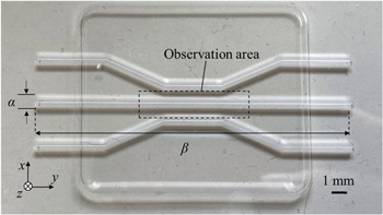
Fig. 1. (Color online) Observation area in an artificial blood vessel for the measurement of the relationship between the concentration of T-cells and brightness of microscopic images.
Download figure:
Standard image High-resolution imageHere, defining the concentration of the cells as C and the volume of the path as V, the area density of the cells contained in the path was calculated as CV/αβ. The number of the cells was obtained by integrating the above area density in the whole path. Considering a x–y coordinate in the obtained fluorescent image, the number of the cells N in the path should be

where Cij indicates the concentration of the cells in the pixel (i, j), and γ indicates the area of a pixel. In this equation, because the parameters of N, V, γ, α, and β are known by the examiner, if the path is filled with a suspension and the brightness on the fluorescent image is regarded to be uniform, then the relationship between mean brightness B and mean the concentration 〈Cij 〉 should be derived, where 〈 〉 indicates the average in the observation area.
2.2. Experimental setup for retention of BSCs
We have designed the experimental setup 11,12) to observe the behavior of the BSCs in flow under ultrasound exposure. Figure 2 shows the vertical view of the experimental setup including the same fluorescence microscope and digital camera, a two-dimensional array transducer, a water tank, and the artificial blood vessel. The transducer, which has a central frequency of 3 MHz and 128 elements, 28) was installed at the bottom of the water tank and targeted the observation area with a distance of l = 60 mm. The elevation angle θ was set to 60° such that the irradiation area of the acoustic field was included in the observation area. The artificial blood vessel was placed at the water surface. In the following experiments, the concentrations of the cells and bubbles were fixed to be 1.0 × 10⁵ ml−1 and 0.3 mg ml−1 in the suspension, respectively, a condition in which we confirmed, under the microscopic images using a confocal microscope, that a cell was fully covered by bubbles. 30) Under the artificial flow of PBS through the artificial blood vessel, a 0.5 ml suspension of BSCs was injected at a point 350 mm upstream from the observation area during ultrasound irradiation, where a duration of ultrasound emission was fixed at 30 s. We chose the velocity range 10–30 mm s−1 because the flow velocity near the main hepatic artery was assumed to be approximately 100–200 mm s−1. Then the cloudy adhesion of BSCs on the upper wall of the path was observed in the middle of the observation area to evaluate the retention performance of BSCs. The number of the retained cells was obtained by a conversion from the brightness of acquired images using Eq. (1) and image analysis software (Nippon Roper, Image pro plus).
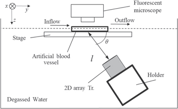
Fig. 2. Experimental setup to observe the behavior of BSCs in flow under ultrasound exposure.
Download figure:
Standard image High-resolution imageTo investigate the method of ultrasound emission to retain as many cells as possible, we applied the tempo-spatial division emission, 28) which moves the position of a single focal point electrically by changing the delay time, in the observation area. Figure 3 shows the positions of the focal points, which move repeatedly from f1 to fn , where the value n indicates the number of focal points. Because the driving equipment (Microsonic ES1144-1) generates a burst wave with a maximum duty ratio of 60%, pulse repetition time was fixed at 1.7 ms, where a continuous wave was emitted for 1.0 ms in each period. For when the number n is more than 2, the transition rate v [mm s−1] between the focal points, which is defined by dividing the distance r [mm] by te , where te indicates the emission duration in each focal point.

Fig. 3. Position and spatial intervals of multiple focal points in the path of the artificial blood vessel.
Download figure:
Standard image High-resolution image2.3. Calculation of applied acoustic intensity
As mentioned in the previous section, the distribution of acoustic intensity on the path varies according to the number of focal points and the magnitude of sound pressure. Therefore, to evaluate retained cells quantitatively, we defined and calculated the applied acoustic intensity of tempo-spatial division emission by measuring actual acoustic fields. Figure 4 shows an example of an acoustic field of a single focal point, where the distribution was divided into small grid areas, with a width w. Also, defining mean sound pressure as Pij [Pa-pp] in a small area, Sij , the applied acoustic power E can be calculated by
where Z is an acoustic impedance of the medium. The coefficient 0.6/n was chosen because the duty ratio per focal point was limited to 60% for the equipment, as mentioned in the previous section.
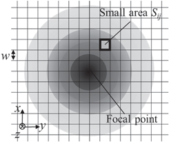
Fig. 4. Schematic of the sound pressure distribution and division in small areas.
Download figure:
Standard image High-resolution imageGenerally, since acoustic power increases in proportion to the exposed area, it is necessary to normalize it by the area, as well as spatial average temporal average intensity, in order to compare between various acoustic fields. In addition to the evaluation of thermal effects caused by high-intensity focused ultrasound, we defined the applied acoustic intensity as I = E/S, where S indicates the area of the acoustic field, which is defined by the area where the relative amplitude is more than −20 dB of the focal point. 31) For the calculation of both E and S, an identical coordinate of w = 0.5 mm was used.
3. Results
3.1. Relationship between concentration of T-cells and brightness
As mentioned in Sect. 2.1, we prepared multiple suspensions, with various concentrations of the cells ranging from 1.0 × 10⁵ ml−1 to 90.0 × 10⁵ ml−1, and concentration of bubbles set to 0.3 mg ml−1, to investigate the relationship between the mean brightness of the fluorescent image and the concentration. Figure 5(a) shows three fluorescent images of the suspension-filled paths without flow, where the concentrations are 100, 400, and 800 × 104 ml−1 under the microscope settings of an 8x gain and 80 ms exposure time. A Plan-Apochromat 1.25x objective lens (NA 0.04, Olympus) was equipped with the microscope. The mean brightness was increased in proportion to the concentration of the cells. Figure 5(b) shows the relationship between the concentration 〈Cij 〉 and brightness B, where the brightness saturated when 〈Cij 〉 was more than 800 × 104 ml−1. From this result, we derived the correlation equation by fitting a quadratic function between 〈Cij 〉 and B. Here it should be mentioned that the brightness threshold was set at 20 because of the background magnitude, which means that concentrations less than 38.8 × 10⁴ ml−1 were ignored for the cell counting using Eq. (1).
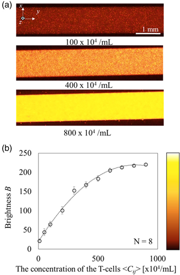
Fig. 5. (Color online) The relationship between the concentration of T-cells and brightness on the microscopic images. (a) The fluorescent images filled with the suspension of T-cells and bubbles, and (b) the relationship between the concentration of T-cells 〈Cij 〉 and mean brightness B of the fluorescent images.
Download figure:
Standard image High-resolution image3.2. Estimation of applied acoustic intensity of acoustic field
Before applying tempo-spatial division emission of a focal point, as mentioned in Sect. 2.3, we measured the sound pressure distributions of various acoustic fields with multiple focal points using an acoustic intensity measurement system (Onda AIMS III) by translating the hydrophone (Onda HNR-1000) in degassed water. Figure 6 shows the profiles of the applied acoustic intensity when the number of focal points was n = 1, 2, 3, and 4, with spatial interval (a) r = 2 mm and (b) r = 3 mm, along the y-axis of the path as shown in Fig. 3. Figure 7 shows the special distribution of the applied acoustic intensity in x–y plane. These distributions were measured individually to superimpose the identical coordinates. Note that although the maximum sound pressure of each focal point was adjusted to 400 kPa-pp, the peak value of the applied acoustic intensity varied according to the number of the focal points because of tempo-spatial division emission.
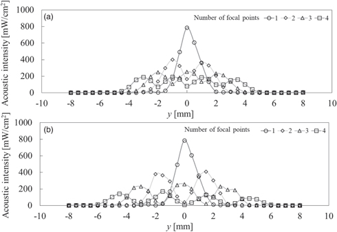
Fig. 6. Spatial distribution variation on y-axis of acoustic intensity including multiple focal points with spatial intervals (a) r = 2 mm and (b) r = 3 mm.
Download figure:
Standard image High-resolution image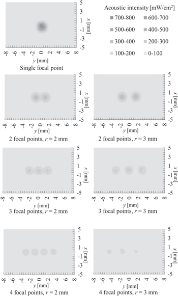
Fig. 7. Spatial distribution variation on xy-axis of acoustic fields including multiple focal points with spatial intervals of 2 and 3 mm.
Download figure:
Standard image High-resolution image3.3. Verification of the transition rate of focal points
Before verifying the parameters of the acoustic field shape, we investigated the effect of the transition rate of the focal points produced by the previously mentioned tempo-spatial division emission. By fixing the ultrasound emission conditions of the three focal points (i.e. spatial interval r of 3 mm, maximum sound pressure of 400 kPa-pp realized with a two-dimensional array transducer, and flow velocity of 10 mm s−1), we examined to retain the BSCs at different transition rates from 10 to 1000 mm s−1. Figure 8 shows the number of retained T-cells versus the transition rate; the error bars indicate the standard deviations. The number of retained cells was maximal when the transition rate was 100 mm s−1; thus, a transition rate that is 50 times faster than the flow velocity does not effectively propel the cells. Therefore, we fixed the transition rate at v = 100 mm s−1 in the following experiments to determine which other parameters can retain cells. Under this condition, because the emission duration te in each focal point was 30 ms, the repetition time for the three focal points was 90 ms. As the total duration of the ultrasound emission process was 30 s (Sect. 2.2), the transition of the focal points was repeated more than 300 times.
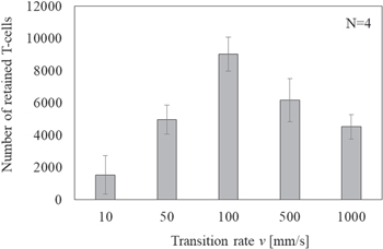
Fig. 8. Calculated number of retained T-cells versus transition rate v with a maximum sound pressure of 400 kPa-pp and flow velocity of 10 mm s−1.
Download figure:
Standard image High-resolution image3.4. Verification of the spatial interval of focal points
As mentioned in the above section, the distribution of sound pressure depends on the spatial interval of the focal points. Here, we compare the retained number of the cells with two different spatial intervals with multiple focal points using tempo-spatial division emission. The acoustic field was produced with three focal points and a maximum sound pressure of 400 kPa-pp, which are shown in Fig. 6. Figure 9 shows the fluorescent images of the retained BSCs with a flow velocity of 10 mm s−1 taken 30 s after the injection of the suspension. In both spatial intervals, although the cells were not confirmed near the first focal point f1, clouds of the retained cells were seen near f2 and f3. However, when the spatial interval was set to 3 mm, there seemed to be lack of retained cells between f2 and f3, which corresponds to the distribution of sound pressure shown in Fig. 9.
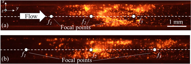
Fig. 9. (Color online) The fluorescent images of retained BSCs on the upper wall of the path under the exposure of three focal points with a maximum sound pressure of 400 kPa-pp, where the spatial intervals were (a) r = 2 mm, and (b) r = 3 mm with a flow velocity of 10 mm s−1, at the moment after starting ultrasound emitted for 30 s.
Download figure:
Standard image High-resolution imageFigure 10 shows the calculated number of retained cells versus the number of focal points with a maximum sound pressure of 300 kPa-pp according to flow velocities. The error bars indicate the standard deviation. The number of retained cells showed the maximum when two or three focal points were applied with a spatial interval of r = 2 mm and a flow velocity of 10 mm s−1. Also, it is obvious that the number of retained cells significantly decreased with spatial interval r = 3 mm with every number of focal points. Considering the above results, we fixed the spatial interval r = 2 mm in the following experiments to verify other parameters to retain more cells.
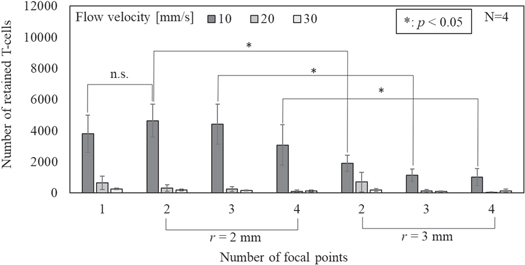
Fig. 10. Calculated number of retained T-cells versus the types of acoustic field with a maximum sound pressure of 300 kPa-pp according to flow velocity.
Download figure:
Standard image High-resolution image3.5. Verification with flow velocity, acoustic intensity, and the number of focal points
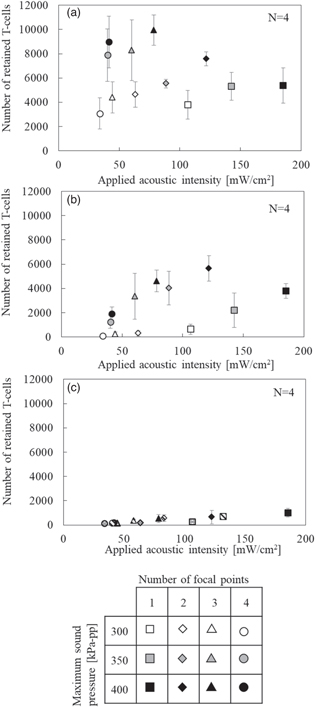
We investigated similar retention performances by varying the flow velocity, maximum sound pressure, and number of focal points in tempo-spatial division emission. the retained number of the cells increased in proportion to sound pressure. Figure 11 shows the number of retained cells versus the applied acoustic intensity according to the maximum sound pressure, number of focal points and flow velocity. Regarding Figs. 11(a) to 11(c), with flow velocities of (a) 10 mm s−1, (b) 20 mm s−1 and (c) 30 mm s−1, the retained number of the cells increased in proportion to applied acoustic intensity. Comparing the results when the maximum sound pressure was 400 kPa-pp, in Fig. 11(a), a maximum number of 10 000 cells was retained with three focal points, where 80% of the ultrasound-exposed cells was retained in the path. On the other hand, in Fig. 11(b), 6000 cells were retained with two focal points, despite the acoustic condition in the horizontal axis in Fig. 11 being common in all results. Then the maximum retention performance was confirmed with an applied acoustic intensity of 40–80 mW cm−2 with a flow velocity of 10 mm s−1, whereas the applied acoustic intensity of 120 mW cm−2 was the maximum with a flow velocity of 20 mm s−1. Also, the number of retained cells varied with applied acoustic intensity in higher number of focal points, where the multiple focal points with an acoustic intensity of 50–120 mW cm−2 were more effective than the single focal point with 180 mW cm−2 in the range of a flow velocity of 10–20 mm s−1.
Fig. 11. Calculated number of retained T-cells versus applied acoustic intensity according to flow velocity of (a) 10 mm s−1, (b) 20 mm s−1, and (c) 30 mm s−1.
Download figure:
Standard image High-resolution image
4. Discussion
In this research, we evaluated the retained cells on the walls of the path quantitatively, derived from the relationship between the concentration of the cells and brightness of the fluorescent images as shown in Fig. 5(b), under the exposure of acoustic radiation force formed with tempo-spatial division emission. In the settings of the fluorescent microscope we used in this experiment, because the brightness saturated at 210, there might be an error in the number of the cells in highly concentrated areas with more than 800 × 104 ml−1 in the retained aggregation. To validate the relationship between the concentration and the brightness, we estimated the number per 1 mm2 with the concentration of 800 × 104 ml−1. First, because the size of a cell is estimated to be around 120 μm2, the maximum area density of the cells is estimated to be about 8500 mm−2 in the observation area. Using the concentration of the cells at 800 × 104 ml−1, with a depth of 1 mm, width α = 1 mm and length β = 80 mm of the path, the cells were found to be distributed with an area density of 8000 mm−2, if they are uniformly distributed, and to occupy more than 90% of the observation area. Therefore, although there is a limitation in the layered cells, the estimation of number of the cells is considered to be quantifiable using the dispersed cells.
In Sect. 3.3, we present the evaluation of the retention performance at 10 mm s−1 flow velocity at different transition rates in different acoustic fields with three focal points, a spatial interval r of 3 mm, and maximum sound pressure of 400 kPa-pp. We chose a transition rate of 100 mm s−1 to determine the retention performance in the following experiments; transition rates of more than 500 mm s−1 significantly degraded the retention performance. Because the beam width of a focal point was estimated to be approximately 2 mm (as shown in Fig. 6), a BSC could pass through a focal point in 200 ms. When the transition rate was 500 mm s−1 (as mentioned in Sect. 2.2), the calculated emission duration te per focal point was 6 ms. When the transition rate was 100 mm s−1, the emission duration was 30 ms, which might is critical for determining the retention performance under these conditions. We are going to present a method for deriving the optimal transition rate according to the flow velocity based on these results.
In Sect. 3.4, the retention performance was evaluated using various acoustic fields, which have multiple focal points with different spatial intervals in their ultrasonic sound fields. At a flow velocity of 10 mm s−1 and a sound pressure of 300 kPa-pp, there was a significant difference between the two types of spatial intervals, where, with three focal points, the number of retained cells in r = 2 mm was 3.9 times higher than that in r = 3 mm. According to the comparison of the acoustic intensity distributions with three focal points in Fig. 6, despite the fact that the maximum acoustic intensity was 250 mW cm−2, the minimal acoustic intensity between focal points with r = 2 and 3 mm were about 100 and 25 mW cm−2, respectively, which indicates that a longer distance of 1 mm between the focal points decreased 74% of the retained number of the cells. Since a subsidence in acoustic intensity distribution reduces the retention performance of the cells, we considered that an evenness in sound field distribution is important for the retention performance of the cells.
In Sect. 3.5, the retention performance was evaluated by varying the flow velocity, maximum sound pressure, and number of focal points. As shown in Fig. 11, the number of retained cells increased in proportion to the applied acoustic intensity along the same focal points. However, with the same maximum sound pressure, the number of retained cells varied depending on the number of focal points. At a flow velocity of 10 mm s−1 and a maximum sound pressure of 400 kPa-pp with three focal points, the number of retained cells was 1.6 times higher than that with a single focal point. As the number of focal points increased, the applied acoustic intensity in each focal point decreased because of the tempo-spatial division emission to enlarge the exposed area. Therefore, even at the same sound pressure, the number of retained cells was affected by multiple parameters as shown in Fig. 11. If bubble oscillation is the dominant factor of this phenomenon, it is likely that there is an optimal duration for bubbles attached to the cells to take effect; this indicates that a short duration, due to emission interruption, is insufficient for generating an acoustic radiation force, whereas a long duration might lead to the collapse of bubbles. Furthermore, the number of focal points needed to obtain the maximum number of retained cells depends on the flow velocity. When the ultrasound irradiation system and presented artificial blood vessel are used at a flow velocity above 20 mm s−1, even if the intensity is spatially dispersed and the time required to irradiate the cells is prolonged, we assume that the cells have passed the exposure area before reaching the wall surface. To retain a certain amount of the cells at a higher flow velocity, a higher acoustic applied intensity is required, therefore it is important to reduce the number of focal points according to the condition of flow velocity.
5. Conclusions
In this study, we first obtained a relationship between the concentration of the cells and brightness of BSCs in an artificial blood vessel observed using a fluorescent microscope. Then, applying a method for calculating the number of retained cells from fluorescent images, we compared the retention performance by using two types of acoustic fields with different spatial intervals between focal points under the exposure of the tempo-spatial division emission. Since we realized that an evenness in sound field distribution was important for the retention performance of the cells, we chose the acoustic field with narrower spatial intervals between the focal points. Furthermore, we evaluated the retention performance through various conditions of the flow velocity, applied acoustic intensity, maximum sound pressure, and number of focal points. Under a lower flow velocity, it was possible to increase the number of focal points with higher sound pressures and expand the exposure area. On the other hand, it has been found that it is important to reduce the number of focal points as the flow velocity increases, to ensure the required acoustic intensity.
Acknowledgments
The authors express a great thankfulness to Dr. Takashi Mochizuki, in Medical Ultrasound Laboratory, Japan, for technical advice. This research was supported by a grant from the Japan Society for the Promotion of Science (JSPS) through KAKENHI Grant Number 20H04547.