
Abstract
Visualization of dermal circulation is important in the field of skin healthcare. We have developed a three-dimensional (3D) photoacoustic (PA) imaging system using a spherically curved array transducer that can visualize the microscale circulation in the skin layers, but limited anatomical information was available around the microvasculature. To provide such anatomical information, this study was aimed at devising a high-quality and high-speed ultrasound (US) imaging framework, particularly, for the spherical array transducer. We tested three synthetic transmit aperture (STA) methods, all-elements, outer-track, and inner-track, for transmission by evaluating the spatial resolution and uniformity of 3D images of point and copper-wire targets. The results demonstrated that the all-elements and outer-track STA methods could provide uniform and clear 3D images. In addition, the outer-track STA could be performed with fewer transmissions than the all-elements STA, and it will be useful for realizing real-time, high-resolution 3D PA/US imaging.
Export citation and abstract BibTeX RIS
1. Introduction
Dermal healthcare is vital to various medical fields. It is useful in the treatment of skin diseases and aging, and for peripheral circulation. 1,2) The structure and characteristics of the microvessels present in the dermal layer (0.1–2 mm in depth from the skin surface), which supply nutrients to skin cells, are the key factors in determining dermal conditions. 3) To precisely elucidate the changes in the characteristics of microvessels, microscale imaging of the dermal layer plays an important role. Photoacoustic (PA) imaging techniques have attracted considerable attention in recent years as a modality that can provide high-contrast and selective microvascular images of the skin layers. Essentially, the PA-imaging modality acquires PA signals propagated from particles that absorb energy applied from nano-seconds laser pulses and generate acoustic waves based on the "photoacoustic effect." 4,5) Since the intensity of the PA waves is proportional to the amount of energy absorbed by the particles, selective blood-vessel imaging is possible if the laser wavelength is adjusted to the optical property of the red blood cells.
PA imaging can be classified based on spatial resolution and image reconstruction methods, such as optical-resolution PA microscopy (OR-PAM), 6–8) acoustic-resolution PAM (AR-PAM), 9–11) and PA tomography (PAT). 12–19) Although OR-PAM has a high spatial resolution of approximately 10 μm, it can only observe structures near the surface (<1 mm). On the other hand, AR-PAM provides a deeper penetration depth of >1 mm, but the spatial resolution is inferior (∼30 μm). In addition, both PAM methods generally have slow imaging speeds owing to mechanical scanning, and this makes their biological interpretation difficult in in-vivo imaging. In contrast, PAT does not require a mechanical scan because it employs multi-element ultrasound array transducers and performs volumetric data acquisition at once with a single laser emission and multi-element PA reception. Therefore, PAT can achieve a high volumetric acquisition rate of 10 Hz with a typical spatial resolution of 200 μm. In previous studies, we have developed a PAT-based PA imaging system equipped with a custom-designed spherically-curved array transducer to achieve three-dimensional (3D) PA images with high spatial and temporal resolution, and we have successfully visualized skin microvessels in a 2 × 2 × 2 mm volumetric space. 20) However, the obtained PA images lacked anatomical information around the vessels. Because the signal reception mechanism of PA imaging is the same as that of ultrasound (US) imaging, it should be possible to use the transducer for US imaging as well to acquire the morphological information of the tissue and complement the present limitation.
Recently, many studies on integrated PA and US imaging systems (PA/US imaging) have been reported. 21–27) However, the characteristics of the transducers used in these studies are different from that used in our study; our transducer (i.e., a spherically curved array transducer) has a hemispherical shape and 256 considerably large (approximately 2.2 × 2.2 mm) elements owing to the priority given to the reception sensitivity for PA signals. When this transducer is used for US imaging, the characteristics of the element and its arrangement provide significantly strong directivity of the ultrasonic waves and generate grating and side lobes that deteriorate the B-mode image quality. Therefore, it is important to determine the optimal US imaging sequence, particularly for a spherically curved array transducer.
In our recent study, we tested the performance of the synthetic transmit aperture (STA) method for US imaging using the spherically curved array transducer. 28) STA is an ultrasound imaging scheme that performs multiple "single-element transmission and full-elements receiving," changing the transmit element and compounding the beamformed signals from each transmit–receive event to construct a high-resolution image. 29–31) We confirmed that the STA method improved the 3D-imaging quality of the spherically curved array transducer better than the single-time "single-element transmission and full-elements receiving" imaging. Nevertheless, the STA method has a trade-off relationship between the image quality and the acquisition frame rate; thus, it is necessary to further consider the optimal selection of transmission elements to achieve sufficient image quality and frame rate.
In this study, we compared the 3D US-imaging quality of three STA schemes with different combinations of transmit elements in a spherically curved array transducer by conducting the following three experiments. First, we estimated the imaging performance of the STA methods by simulating the transmitted acoustic field and echo signals from point scatterers. Next, using the actual transducer, a single-wire phantom was imaged to evaluate the image quality near the geometrical focal point. Finally, five-wire phantoms were placed in a 3D space and imaged to evaluate the performance of the 3D imaging.
2. Experimental methods
2.1. Spherically curved array transducer
This study used a custom-designed spherically curved array transducer (JAR831, Japan Probe Co., Ltd., Kanagawa, Japan), as reported previously. 20) The center frequency and fractional bandwidth of the transducer were 11.5 MHz and 62% (8–15.5 MHz), respectively. This transducer was designed to maximize the sensitivity to PA waves by considering the following three factors: (1) A large solid angle of the ultrasonic detector aperture; (2) a wide bandwidth and high center frequency of the ultrasonic detector, reasonably matching those of the PAS; and (3) a reasonably low electrical impedance of the ultrasonic detector to avoid impedance mismatch between the cable and preamplifier. In this study, this transducer was used for US imaging to achieve the project goal of duplex PA/US imaging.
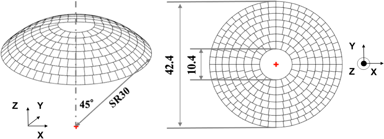
As shown in Fig. 1, the transducer consists of 256 square-shaped PZT elements (element size: approximately 2.2 × 2.2 mm) distributed on a hemispherical surface divided into seven concentric tracks with even widths. 28) The outer diameter, aperture angle, and spherical radius of the hemispherical geometry were 42.4 mm, 90°, and 30 mm, respectively. In addition, a hole of 10.4 mm diameter was made in the center of the transducer for laser irradiation during PA imaging. In this study, we defined the origin of the 3D-imaging space as the geometric focal point of the transducer and the z-axis as the line from the origin to the center of the transducer. Accordingly, the x and y axes formed the 2D plane perpendicular to the z-axis (Fig. 1).

Fig. 1. (Color online) Dimensions of the spherically curved array transducer. SR: spherical radius. All values are in mm. 28)
Download figure:
Standard image High-resolution imageAs mentioned previously, each element of the spherically curved array transducer has a large area and is expected to have strong directivity. We conducted a sound-field simulation to determine the ultrasonic-irradiation range when ultrasonic waves are transmitted from one of the 256 elements. Assuming that a transducer element is composed of multiple small areas dS and each dS transmits a continuous sound wave to a point (x, y, z) in the imaging space, the acoustic-field profile  formed by the entire transmit element can be expressed as follows:
32)
formed by the entire transmit element can be expressed as follows:
32)

where ρ is the density of the propagating medium, α is the volumetric acceleration, ω and k are the angular frequency and the wave number of the emitted ultrasonic wave, respectively, t is the time, r is the distance between an element dS and a point (x, y, z), and S is the surface area of the transducer element. In the simulation, the propagation medium and time elements in Eq. (1) were neglected, and the acoustic field profile was obtained only from the surface integral to estimate the spatial range covered by the transmitted wave from one element.
Figures 2(a) and 2(b) show the simulated acoustic field in the mid x–y plane and mid x–z plane, respectively, when 12.5 MHz acoustic waves are transmitted from an element in the inner most track of the spherical array transducer. In addition, Figs. 2(c) and 2(d) show the acoustic field profile when an element in the outermost track is used for transmission. The visualization areas (normalized intensity > 0.5) of inner- and outer-track elements in the mid x–y plane were found to be 1.6 mm × 2 mm and 1.5 mm × 1.9 mm, respectively; thus, both visualization areas are almost identical [Figs. 2(a) and 2(c)]. In contrast, the acoustic field profile in the axial direction [Figs. 2 (b) and 2(d)] demonstrated that the ultrasound beam angle corresponded to the element location, suggesting that the spatial uniformity of 3D-US imaging may change depending on the transmitting elements used in the STA method.
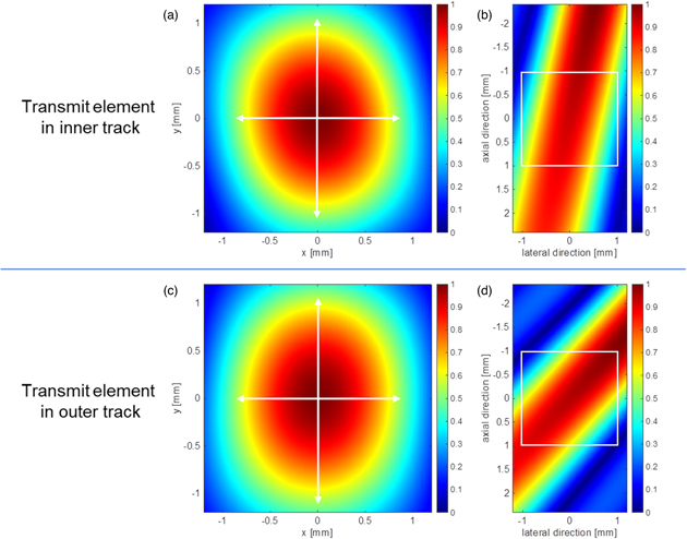
Fig. 2. (Color online) The spatial profile of the transmit beam from an element in the most inner-track derived in the sound field simulation in the x–y plane (a), (c) and in the y–z plane (b), (d).
Download figure:
Standard image High-resolution image2.2. Synthetic transmit aperture (STA) method
The STA method
30,31,33) was used as a US imaging scheme to enhance image clarity and uniformity. In this method, acoustic pulses are transmitted from only one element in the transducer, and the echoes are received by all the M elements assembled in the transducer. This transmit-receive event is repeated for N transmit elements, resulting in the acquisition of N × M echo signals. Dynamic receive-focusing was performed by calculating the delay time, which depends on the geometric distance from the transmitting element ( ) to the imaging point (
 ) and the distance back to the receiving element (
 ), as shown in Fig. 3. The round-trip delay
  for an acoustic pulse emitted from element m, reflected from the object, and received by element n can be calculated as


where r is the focal length (distance from each element to the geometric focus), c is the speed of sound,  and
and  are the distances to the image point from the transmitter and receiver elements, respectively. Using the delay time, the amplitude of the echo signal from an image point (
 ) was calculated by beamforming the received signal at all M elements and compounding the beamformed signal over N transmission as follows:

where  is the echo signal, and
  is the delay time calculated using Eq. (2). The number of transmissions (N) used in the STA method has a trade-off relationship between the image quality and acquisition frame rate; thus, it is necessary to consider the optimal selection of transmission elements to achieve both sufficient image quality and frame rate. In this study, we devised a new method in which a specific transmission pattern of the elements was selected, and the process of transmitting and receiving was repeated for the selected elements. The process of transmitting a US with one element to obtaining the signal at the imaging point was the same as in the STA methods. Three transmission patterns, i.e. all-element, outer-track, and inner-track STA, used respectively 256, 52, and 20 elements for sequential transmissions as shown in Figs. 4(a)–4(c). Because the uniformity of ultrasonic irradiation may differ depending on the track where the element is located, we selected the inner-track STA and outer-track STA as the transmission patterns with a small number of transmit-receive events. The outer-track STA had a larger transmission angle than that of the inner-track STA and was expected to irradiate ultrasonic waves more uniformly. In the imaging sequence, the all-elements STA method was designed to repeat the "one-element transmission and full-element receiving (1chTx-256chRx)" event 256 times, changing the transmission element one by one, and an image was reconstructed using Eq. (4). Similarly, the outer-track STA and the inner-track STA methods repeated the "1chTx-256chRx" event 52 and 20 times, respectively, using the elements painted in blue in Figs. 4(c) and 4(d) for the sequential transmissions.

Fig. 3. (Color online) A schematic of the spatial relationship among the transmit element, the receive element and the image point for calculating the delay time. 28)
Download figure:
Standard image High-resolution image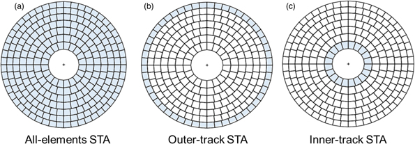
Fig. 4. (Color online) Location of the transmit elements for each method. "All-elements STA," "Outer-track STA," and "Inner-track STA" methods performed multiple "one-element" transmissions sequentially using an element in those filled in blue. After each transmit event, echo signals were received at all 256 elements for dynamic receive focusing and compounding over the transmissions.
Download figure:
Standard image High-resolution image2.3. Experimental setup
Figure 5 shows the setup used in the experiment. The US signals were acquired using a programmable ultrasound platform (Vantage 256, Verasonics Inc.) with 256 independent transmit and receive channels. In this study, one cycle of 12.5 MHz transmit pulse was used, and the echo signals were acquired at a sampling frequency of 62.5 MHz. The acquired US signals were processed and analyzed in MATLAB (MathWorks, Natick, USA).
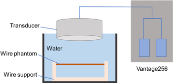
Fig. 5. (Color online) Experimental setup.
Download figure:
Standard image High-resolution imageFirst, we performed simulations to estimate the 3D-imaging performance of the proposed STA methods using the simulation mode of Vantage 256. As shown in Fig. 6, a total of 27 point scatterers were placed at 0.9 mm intervals in a volumetric space of 2 × 2 × 2 mm. The center point of the volumetric space was set to the geometric focal point of the transducer. Because the Vantage 256 simulation mode does not consider the element size of the transducer, we resembled the transmit beam generated by an element of our transducer by distributing 100 points of acoustic sources in the area of a selected transmit element and synchronously activating the acoustic sources. Figure 7 depicts the spatial profile of the transmitted pulse simulated in the Vantage simulation, which is similar to that shown in Fig. 2. During reception, the echo signals were virtually received at each center point of all 256 elements. Using the simulated echo data, the three imaging methods shown in Fig. 4 were used. The full width at half maximum (FWHM) was calculated from the envelope to evaluate the axial and lateral resolutions. In addition, the standard deviation of the intensity of the visualized scatterers was calculated to evaluate the uniformity of each imaging method.
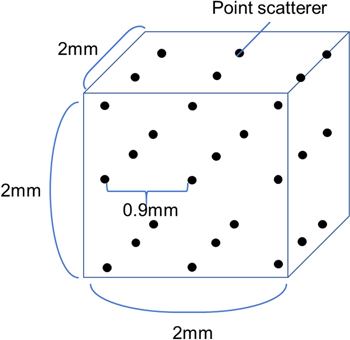
Fig. 6. (Color online) Simulation experiment.
Download figure:
Standard image High-resolution image
Fig. 7. (Color online) The spatial profile of the transmitted pulse simulated in the Vantage simulation in the x–y plane (a) and in the y–z plane (b).
Download figure:
Standard image High-resolution imageNext, to investigate the resolution and imaging performance of the actual imaging in a simple case, echo signals from a copper wire of 100 μm diameter placed in water at a depth of 30 mm, which was the geometric focal depth of the transducer, were acquired using the actual transducer and a Vantage 256 system (hereafter called 2D-wire phantom experiment). C-mode and B-mode images were generated using the three methods described in Sect. 2.2, and the FWHM of the copper wire in the images was calculated to evaluate the axial and lateral resolutions.
Finally, to evaluate the performance of each method in 3D imaging, imaging was performed using five copper wires of 100 μm diameter placed in a crisscross pattern in water within a 2 (lateral) × 2 (depth) mm area, including the focal point, as shown in Fig. 8 (hereafter called 3D-wire phantom experiment). The three methods were tested to generate C-mode and B-mode images, and a 3D volume image. Similar to the simulation tests, the FWHM of the copper wires in the images was calculated to evaluate the axial and lateral resolutions, and the standard deviation was calculated from the intensity of the visualized five copper wires to evaluate the uniformity of the actual volumetric imaging.
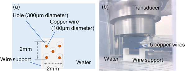
Fig. 8. (Color online) 3D wire phantom experiment. (a): diagram, (b): picture.
Download figure:
Standard image High-resolution image3. Results and discussion
3.1. Vantage 256 simulation
Figure 9 shows the imaging results obtained from the simulation. In the B-mode image, the outer-track STA is slightly larger in the axial direction than the all-elements and inner-track STAs. In the C-mode image, the image obtained by the outer-track STA, as shown in Fig. 9(e), is smaller in the lateral direction than that obtained by the all-elements STA, as shown in Fig. 9(d). On the other hand, the image obtained by inner-track STA showed wider point targets, as shown in Fig. 9(f), than that of the all-elements STA. In addition, in all the images, the reflectors located at the edges were imaged darker than the reflectors at the center. The FWHM was calculated from the envelope of the dotted line in Fig. 9, and the mean and standard deviation of the signal intensity at each point are listed in Table I. The outer-track STA showed the minimum resolution of 77.5 μm. In contrast, the axial resolution was found to be the smallest in the inner-track STA, and it increased in the all-elements and outer-track STAs. Among the STA methods, the outer-track STA showed a slightly lower standard variance in the spatial signal intensity compared to those of the all-elements and inner-track STA methods.
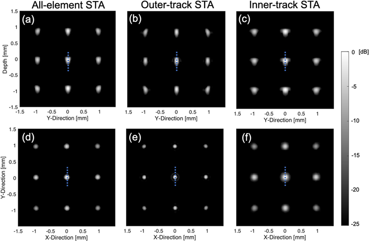
Fig. 9. (Color online) B-mode (a)–(d) and C-mode (e)–(h) images generated from the simulated echo signals using three STA methods.
Download figure:
Standard image High-resolution imageTable I. Spatial resolution and standard division in simulation. All values are displayed in dB.
| All-elements STA | Outer-track STA | Inner-track STA | |
|---|---|---|---|
| Axial resolution (μm) | 128.4 | 138.5 | 122.1 |
| Lateral resolution (μm) | 94.6 | 77.5 | 119.5 |
| Average Intensity ± SD | 115.1 ± 3.1 | 116.7 ± 2.7 | 117.5 ± 3.6 |
3.2. 2D-wire phantom experiment
Figure 10 shows the imaging results of a single copper wire placed at the focal depth. In the B-mode images, the all-elements and outer-track STAs show almost the same imaging performance. The location of the side lobes is slightly different among the three methods. In the C-mode images, both ends of the copper wire in the range of 2 × 2 mm, shown by the blue square, can be imaged by either method. However, the inner-track STA has stronger side lobes near the center of the image than those of the all-elements and outer-track STAs. Table II lists the results of the spatial resolution calculated using the FWHM from the envelope of the dotted line in Fig. 10. The outer-track and all-elements STA methods exhibited better lateral resolutions compared to that of the inner-track STA. The axial resolution was lower in the inner-track STA and increased when the all-elements and outer-track STAs were used. Thus, the changes in the resolution according to the transmission methods agreed with those observed in the simulation experiment.

Fig. 10. (Color online) B-mode (a)–(d) and C-mode (e)–(h) images of 2D wire phantom acquired by three STA schemes.
Download figure:
Standard image High-resolution imageTable II. Spatial resolution in 2D wire phantom experiment. All values are displayed in dB.
| All-elements STA | Outer-track STA | Inner-track STA | |
|---|---|---|---|
| Axial resolution (μm) | 157.6 | 173.2 | 148.4 |
| Lateral resolution (μm) | 82.2 | 72.3 | 97.4 |
3.3. 3D-wire phantom experiment
Figure 11 shows the B-mode and C-mode images of the five-wire phantoms generated in each STA method, and Fig. 12 shows the volume rendering results. The intensity was normalized by the maximum intensity of the volumetric data for each STA method. B-mode images of the all-elements and outer-track STAs [Figs. 11(a)–11(b)] had a similar lateral resolution, while that of the inner-track STA had a stronger sidelobe compared to the those of the other STA methods. This can also be confirmed in the C-mode image of the central wire, as shown in Figs. 11(d)–11(f). In addition, the C-mode images [Figs. 11(g)–11(i)] that display the upper right wire in Figs. 11(a)–11(c)] demonstrate that the all-elements and outer-track STA images provide a sharper view of the wire than the inner-track STA even outside of the focal depth.
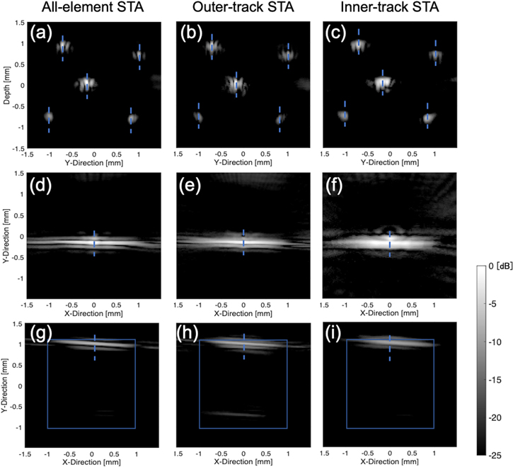
Fig. 11. (Color online) 3D wire phantom images of each transmit scheme. B-mode images (a)–(c) and C-mode images of the upper left wire (d)–(f) and the middle wire (g)–(i) in the B-mode images.
Download figure:
Standard image High-resolution image
Fig. 12. 3D images of the five wires. (a) All-elements STA; (b) Outer-track STA; and (c) Inner-track STA.
Download figure:
Standard image High-resolution imageTable III lists spatial-resolution results calculated using the FWHM from the envelope of the dotted line in Fig. 11. For all the copper wires, the trends in the lateral and axial resolutions were the same as those observed in the 2D-wire phantom experiment. The lateral resolution of the central-wire images with the inner-track STA method increased owing to the strong side lobes. In addition, the all-elements STA and inner-track STA methods exhibited smaller standard deviation values than that of the outer-track STA, which is a different tendency from the simulation results.
Table III. Spatial resolution in 3D wire phantom experiment. All values are in dB.
| All-elements STA | Outer-track STA | Inner-track STA | ||
|---|---|---|---|---|
| Upper right wire | Axial resolution (μm) | 165.6 | 168.3 | 162.5 |
| Lateral resolution (μm) | 67.4 | 68.4 | 112.9 | |
| Center wire | Axial resolution (μm) | 153.5 | 173.4 | 147.9 |
| Lateral resolution (μm) | 72.7 | 69.8 | 186.0 | |
| Signal Intensity | Average±SD | 79.62 ± 4.7 | 78.83 ± 6.08 | 83.65 ± 5.40 |
3.4. Discussion
From the spatial resolution obtained by simulation and 3D imaging, among the three proposed methods, the inner-track STA provided a slightly better axial resolution, while the all-elements and outer-track STAs demonstrated a significant improvement in the lateral resolution. In addition, the inner-track STA exhibited a strong side lobe, which was not significant in the outer-track and all-elements STAs. Therefore, the outer-track STA was capable of achieving a better imaging quality that is similar to that generated in the all-elements STA, while the outer-track STA reduced the number of US transmissions and increase the acquisition-frame rate. Further investigations need to be conducted in the future to validate the effectiveness of the outer-track STA method for in in-vivo imaging.
As mentioned above, in all the three experiments, we observed that there was a slight trade-off between the lateral and axial resolutions between the inner-track and outer-track STAs. In addition, a strong side lobe was observed only in the inner-track STA. These phenomena were ascribed to the difference in the overlapping of signals due to the transmission angle. Figures 13(a) and 13(b) depict the compounded RF signals in the outer-track and inner-track STA imaging. As shown in Fig. 13, the STA transmitting from the outermost track had a wide signal overlap in the axial direction, whereas the inner-track STA had a narrow signal overlap in the axial direction, indicating that the mechanism of the axial resolution in the outer-track STA was slightly larger than that of the inner-track STA, and vice versa, for the lateral resolution. In addition, when the axial overlap is narrower, the side lobes generated in each transmission are likely to be strengthened. In future studies, further consideration can be made using the random element activation strategy 33) to achieve high axial and lateral resolutions as well as high temporal resolvability.

Fig. 13. (Color online) Signal overlap diagram (a) Outer-track STA; (b) Inner-track STA; and (c), (d) overlap pattern diagram. Blue arrows indicate the part where the signals to be enhanced.
Download figure:
Standard image High-resolution image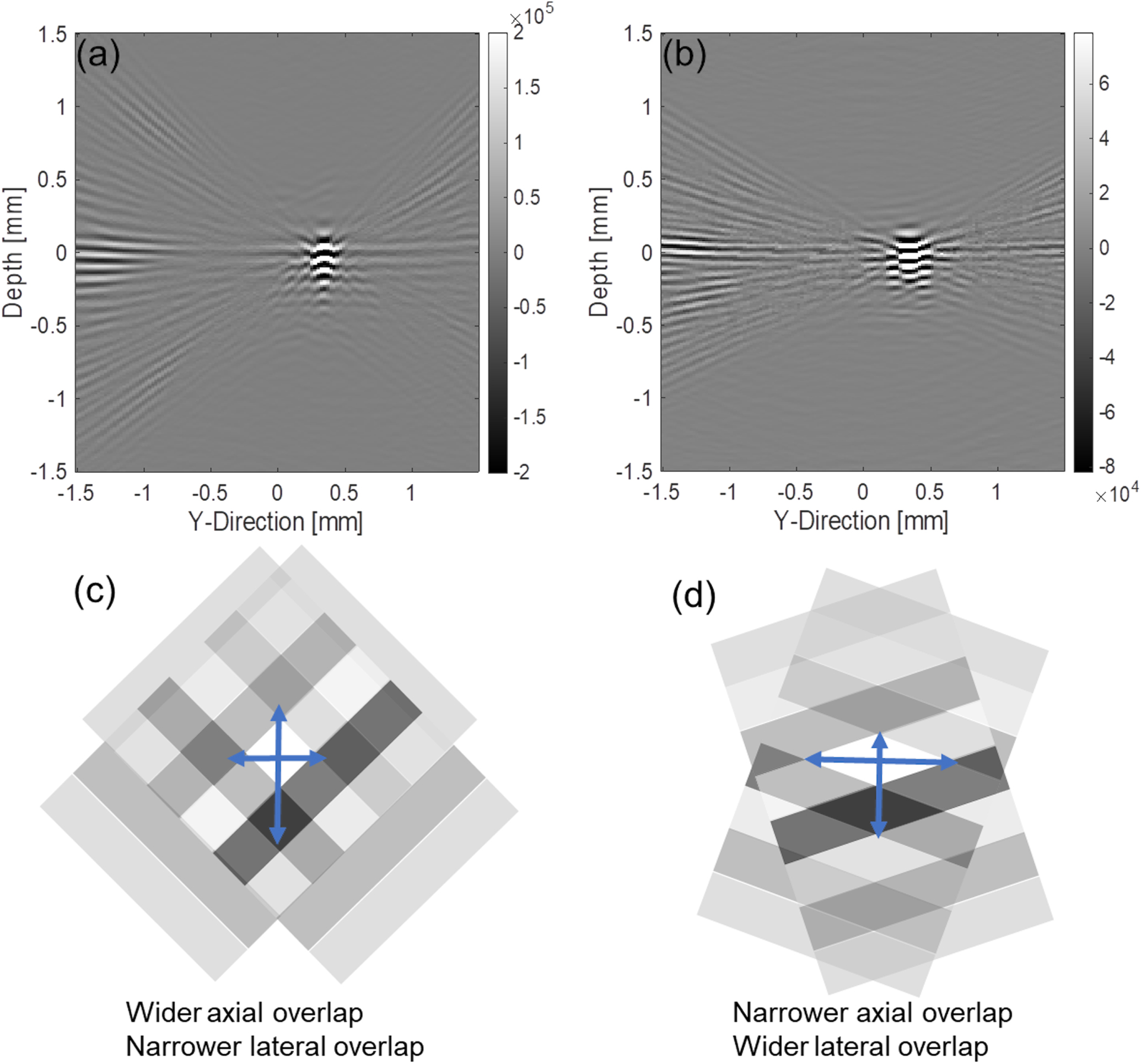
In addition to the improvement in the spatial resolution, another hypothesis was that the outer-track STA irradiates the ultrasonic waves more uniformly than the inner-track STA because the outer-track STA had larger transmit beam angles than that of the inner-track STA. Although this effect was observed in the simulation study, the spatial uniformity in the signal strength was not improved in the actual 3D-wire imaging, and it was observed to be even decreased in the outer-track STA method. This observation might be due to the errors in the transducer-element arrangement (location and direction) produced during the manufacturing of the custom-made transducer. Because the performance of the received beamforming and the coherent compounding in the STA methods relies on the accuracy of the estimated delay time for each signal, the spatial uniformity in the signal strength can be affected if there is a small deviation between the actual element arrangement and the original design. In future studies, a hydrophone measurement can be performed to precisely calibrate the manufactured element arrangement. Note that the effect of the errors in the element arrangement was small enough for the STA methods to successfully suppress the ambient noise, improve the signal-to-noise ratio, and contribute to improving the image quality.
4. Conclusions
In this study, we tested three STA frameworks (all-elements STA, outer-track STA, and inner-track STA) for 3D-US imaging using a spherically curved array transducer, and we evaluated the performance of the transducer in terms of image quality. The simulation and imaging experiments demonstrated that the all-elements STA and outer-track STA methods effectively improve the lateral resolution and suppress the noise components. The two methods provided uniform and clear imaging of the five wire targets closely placed in the 2 × 2 × 2 mm volumetric space; this suggests that it is promising to clearly visualize 3D anatomical features in the layers of the skin. In addition, the outer-track STA method can image with fewer transmissions, achieving a higher frame rate compared to the all-elements STA method. This will be useful for realizing real-time, high-resolution 3D PA/US imaging.
Acknowledgments
This research was partially supported by JSPS Kakenhi Grant numbers 20H04543 and 21H04958.