

Abstract
In epidural anesthesia, it is difficult to specify the puncture position of the anesthesia needle. We have proposed an ultrasonic method to depict the thoracic spine using the different characteristics of reflection from bone and scattering from muscle tissue. In the present paper, we investigated the transmission aperture's width of the ultrasound probe to emphasize the differences in the reflection and scattering characteristics. First, we determined the optimum transmission aperture's width using a simulation experiment. Next, we measured reflection and scattering signals by changing the transmission aperture's width in a water tank experiment and confirmed that the results corresponded to the simulations. However, as the transmission aperture's width increased, the lateral resolution at the focal point improved. Therefore, better imaging of the human thoracic vertebrae can be achieved by selecting the transmission aperture's width, which considers the effect on lateral resolution.
Export citation and abstract BibTeX RIS
1. Introduction
Epidural anesthesia is a local anesthesia method used before surgery, and it is often combined with general anesthesia because it reduces the burden on patients intraoperatively and postoperatively. 1) The anesthesia needle is punctured from the surface of the skin into the spinal space. In epidural anesthesia for the thoracic spine, it is not easy to puncture the anesthesia needle into the proper position because the spinal space is narrow and complex. As the location of the puncture is determined by the physician's palpation at present, the success of anesthesia is dependent on the skills of the physician. The success rate of epidural anesthesia ranges from 75% to 94%, 2–4) and its failure may induce headaches and complications. During epidural anesthesia, patients reported back pain and psychological distress in 22% and 14% of the cases, respectively. 5)
Medical ultrasound confirms the puncture position before anesthesia as an aid of palpation in clinical practice. 6) In epidural anesthesia for the lumbar spine and other regional anesthesia, ultrasound guidance is often used, and its usefulness has been demonstrated. 7–10) However, it is difficult to depict clear images of the puncture position, especially for obese patients with a deep spine or thoracic vertebrae with a narrow gap. 11–13) Several studies have been proposed for the ultrasound guidance of epidural anesthesia, e.g. automatic identification of the spine. 14–16) However, these studies targeted the lumbar spine, which has a wide gap and simple structure.
Ultrasound imaging of bone is studied in the field of orthopedics. 17–20) Several methods have been proposed, e.g. using strain under pressure to identify the bone shape, 21,22) phase symmetry, 23) and shadow peaks. 24) However, it is difficult to apply these methods to the thoracic spine because it is located deep beneath the skin surface and has a complex surface structure.
We have developed an imaging method that can be applied to assist epidural anesthesia in the thoracic spine. In our previous study, we proposed three methods. The first method improves the delayed addition misalignment caused by the reflection of ultrasound at the thoracic vertebral surface, 25) and it depicts a smooth and tilted object by not considering the transmitting and receiving positions as the same, applying the envelope method 26) and range point migration method. 27,28) The second method is based on the difference in ultrasound characteristics between soft tissue and bone, 29) which calculates the ratio of the delayed addition with a wide range along the time direction to the normal one and multiplies it by the brightness value at each point of the image. The third method is based on the difference between the reflection and scattering ultrasound characteristics. 30) This method uses angular amplitude characteristics, which are enveloped amplitudes of signals received by many elements of the ultrasonic probe at the time corresponding to the depth of the target. This method estimates whether the target is a reflector or scatterer by fitting angular amplitude characteristics obtained from the target with the reference data of reflection and scattering characteristics. The difference in the angular amplitude characteristics between reflection and scattering affects the estimation accuracy of the target.
The purpose of the present paper is to investigate the ultrasound transmission condition so that the difference in angular amplitude characteristics between reflection and scattering is more emphasized in the third method. We fundamentally investigated the difference among angular amplitude characteristics and the difference in the width of the transmission aperture. 31) Focusing on the transmission aperture, the effect of the aperture on the angular amplitude characteristics of scattering and reflection was examined by simulation. Based on the results, a better transmission aperture is determined by the simulation. Finally, simulation results were confirmed using water tank experiments.
2. Principle
2.1. Difference of angular amplitude characteristics between scattering and reflection
Figure 1 shows a wave scattered from a point scatterer when a focused wave is transmitted with a linear probe, where  and
and  are the depth of the point scatterer and the lateral position of the
  th received element, respectively,
  shows the center of the probe aperture, and
  is the speed of sound in the medium. The time ranging from transmission at the center element to the receipt of the wave scattered from the point scatterer at the
  th received element,
  is given by

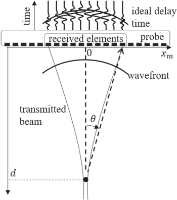
Fig. 1. Transmission and reception of a focused wave by a linear array probe.
Download figure:
Standard image High-resolution imageBy defining the ideal delay time by  and the received signal at
  th element by
  the angular amplitude characteristic
  which shows the head amplitude of the
  just at the ideal delay time
  is provided by the enveloped amplitude
  of
of  as
as

When an ultrasound is irradiated to a scatterer such as muscle tissue, the ultrasound is scattered along with all the directions from the object, which follows Rayleigh scattering when the scatterer is sufficiently smaller than the wavelength of the ultrasound and the angular amplitude characteristic  for the scattering becomes a gentle parabola.
30) On the other hand, when ultrasound is irradiated to a reflector with a regional plate, such as a bone, the ultrasound is specularly reflected, and
for the scattering becomes a gentle parabola.
30) On the other hand, when ultrasound is irradiated to a reflector with a regional plate, such as a bone, the ultrasound is specularly reflected, and  for the reflection becomes high for the direction corresponding to the specular reflection and low for other directions.
30)
for the reflection becomes high for the direction corresponding to the specular reflection and low for other directions.
30)
2.2. Evaluation method for differences in angular amplitude characteristics
The difference between  and
and  was quantitatively evaluated using following the root mean square error (RMSE):

where  is the parameter that minimizes the RMSE. From
  we can determine
  In the present paper, a suitable transmission aperture was determined so that the RMSE becomes maximum for various transmission aperture widths.
2.3. Simulation method
Figure 2(a) shows the simulation done in this paper. The number of received elements was 96, and the element pitch was 0.2 mm, assuming the typical ultrasound diagnostic equipment with the linear probe. When the short axis of a molybdenum wire with a diameter of 30 μm was set in a water tank, the transmitted and received waveform using one element above the wire was measured using ultrasound diagnostic equipment at a center frequency of 7.5 MHz. The waveform sampled at 40 MHz was interpolated 50 times using the sinc function, and the resultant  is shown in Fig. 2(b).
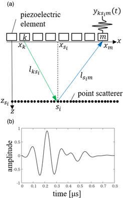
Fig. 2. (Color online) Simulation of the received signal. (a) Calculation of  (b) Received waveform transmitted by one element,
Download figure:
Standard image High-resolution imageThe received signals from a reflector or scatterer were generated when a focused wave with a focal depth of 30 mm was transmitted. In Fig. 2(a),  which is transmitted from the
  th transmitted element, scattered by
  th point scatterer
  and received by
  th received element, is given by

where  shows theoretical scattering characteristics,

and  shows the delay time of propagation from the
  th transmitted element,
  th point scatterer
  and
and  th received element as

where  is the speed of sound in the medium,
  and
and  are the path lengths from the kth transmitting element to
  and from
  to mth receiving element, respectively, and
  is the delay time of the kth element to transmit the focused wave.
  of Eq. (6) comprises the propagation attenuation
  the angular characteristic of Rayleigh scattering
  the reception directivity of piezoelectric elements
  and the effect of interference in the width of the piezoelectric element at the reception of ultrasound,
  32),
32), 
 and
and  are shown in Eqs. (8)–(10), respectively.


where  is the attenuation coefficient of water
  33);
33);  = 7.5 MHz, which is the center frequency of the probe used in the water tank experiments;
  is the scattering angle and is defined as

and  is the incidence angle from the acoustic matching layer to the piezoelectric element given by

where  is the speed of sound in the acoustic matching layer. By considering scattering,
  transmitted from the
  th element and received by the
  th element is given by

By adding  to the transmitted elements
  the received signal at the
  th received element
  is obtained as follows:

In the actual measurement,  is observed at the
  th element and each component of
  cannot be detected. However, by the simulation experiments in the present paper,
  is decomposed into the element signals
  of Eq. (13).
Alternatively in the present paper, we investigated  of Eq. (2) by clarifying the difference of
  between the reflector and scatterer through the simulation experiments for each of the transmission aperture's widths
  (the number
  of transmitting elements) of 19.2 (96 elements), 14.4 (72 elements), 9.6 (48 elements), 4.8 (24 elements), and 0.2 mm (1 element). The signal from a plate reflector was generated by adding all the signals received from point scatterers aligned densely at 20 μm intervals with a width of 50 mm. By aligning point scatterers at 20 μm intervals on a tilted line, the surface of the tilted reflector was simulated.
2.4. Water tank experiments
The ultrasound diagnostic equipment was ProSound SSD-α10 (Hitachi Aloka) with a sampling frequency of 40 MHz. A linear probe UST-5412 (center frequency: 7.5 MHz, number of elements: 192, and element pitch: 0.2 mm) was attached to the ultrasound diagnostic equipment. For transmission, each element was given a delay time so that the focal point was 30 mm, which simulated the depth from the skin surface to the thoracic spine. No apodization was applied for transmission and reception.
Figure 3 shows the water tank experimental system. The short axis of molybdenum wire with a diameter of 30 μm and the surface of an acrylic block were used as a scatterer and a reflector, respectively. The depths of both objects were 30 mm. The angular amplitude characteristics  acquired with changing the transmission aperture's widths
  were compared with the simulation results.

Fig. 3. (Color online) Water tank experimental system. (a) The measurement of the scattering characteristics. The short axis of a molybdenum wire with a diameter of 30 mm was measured as a scatterer. (b) The measurement of the reflection characteristics. The surface of an acrylic block was measured as a reflector.
Download figure:
Standard image High-resolution image3. Results and discussion
3.1. Angular amplitude characteristics of scattering
First, we discuss the simulation results of angular amplitude characteristics  of scattering for a transmission aperture's width (
 ) of 19.2 mm (96 transmitted elements). The received element number of
  at the center position was set to
  mm. Figures 4(a1) and 4(b1) show the received signals
  and
and  at the received positions
  and
and  mm, respectively, for each
  th transmitted element. The dashed lines in these figures show the ideal delay time
  calculated using Eq. (1). By integrating
  and
and  along the direction of the transmitted elements
  Figs. 4(a2) and 4(b2) show the resultant waveforms of
  and
and 
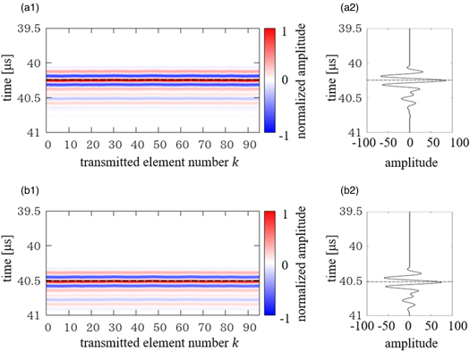
Fig. 4. (Color online) Simulation results of the scatterer. (a1), (b1) Received signals  from each transmitted element. (a2), (b2) Received signals
  (a1), (a2) results for
  mm; and (b1), (b2) results for
  mm.
mm.
Download figure:
Standard image High-resolution imageAs shown in Figs. 4(a1) and 4(b1),  were received at the same time for each received element when the object was a scatterer and placed at the focal point. Thus, the shape of
  was the same as that of the transmitted and received waveform
  based on one element. When the received position
  moved away from above the point scatterer, the signal amplitude in Fig. 4(b2) decreased owing to the receiving directivity of elements compared with that in Fig. 4(a2).
3.2. Angular amplitude characteristics of reflection
Next, we discuss the simulation results of angular amplitude characteristics  of reflection. Figures 5(a1), 5(b1), and 5(c1) show the received signals
 and
and  at
at  and
and  mm, respectively. Figures 5(a2), 5(b2), and 5(c2) show
 and
and  at
at  and
and  mm, respectively. Figures 5(a3), 5(b3), and 5(c3) show the amplitudes of the received signals
 and
and  at the ideal delay time
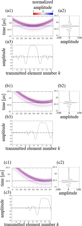
Fig. 5. (Color online) Simulation results of the reflector. The dashed lines represent the ideal delay time  (a1)–(c1) received signal
  from each transmitted element; (a2)–(c2) received signals
  (a1)–(a3) results for
  mm; (b1)–(b3) results for
  mm; (c1)–(c3) results for
  mm.
mm.
Download figure:
Standard image High-resolution imageIn Figs. 5(a1), 5(b1), and 5(c1),  was received earlier than the
  ideal delay time
  when the target was the reflector. This is because the propagation paths are shorter than those when the ultrasound is scattered at the focal point. Therefore, as shown in Figs. 5(a3), 5(b3), and 5(c3), {
 } are not constant for the transmitted elements
The following two things can be found in Fig. 5(a3). The first is that the angular amplitude characteristic  at the central received element
  47 has positively large amplitudes for 24 transmitted elements with
  36–59. The second is that
  is negative for the transmitted elements around
  and
and  By comparing Figs. 5(a3), 5(b3), and 5(c3), the profile of
  moved toward the transmitted elements on the right side. As a result of this movement, the negative components around
  in Fig. 5(a3) were not received at
  as shown in Fig. 5(c3).
3.3. Relationship between the width of the transmission aperture and angular amplitude characteristics
Figure 6 shows angular amplitude characteristics of reflection and scattering when the transmission aperture's width  (the number
  of transmitting elements) was 19.2 (
 = 96), 14.4 (
 = 72), 9.6 (
 = 48), 4.8 (
 = 24), and 0.2 mm (
 = 1). The shape of
  significantly changed as
  decreased, but the maximum value did not significantly change, except when
  = 0.2 mm. On the other hand, the shape of
  did not change, although its amplitude decreased in proportion to the decrease in
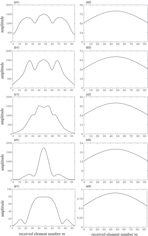
Fig. 6. Simulated angular amplitude characteristics of reflection and scattering for the different transmission aperture. (a1)–(e1) Reflection characteristics; (a2)–(e2) scattering characteristics; (a1), (a2) results for  = 19.2 mm; (b1), (b2) results for
  = 14.4 mm; (c1), (c2) results for
  = 9.6 mm; (d1), (d2) results for
  = 4.8 mm; (e1), (e2) results for
  = 0.2 mm.
Download figure:
Standard image High-resolution imageThis difference is caused by the fact that  for the scattering were almost the same among the transmitted elements [Figs. 4(a1) and 4(b1)], whereas
  for the reflection significantly varied among the transmitted elements [Figs. 5(a3), 5(b3), and 5(c3)]. The decrease in
  corresponds to the exclusion of signals at both ends shown in Figs. 5(a3), 5(b3), and 5(c3).
For reflection, as the received element position ( ) departed from the center, the shape of
  changed [Figs. 5(a3), 5(b3), and 5(c3)], and the transmitted elements
  with large amplitudes of
  shifted toward the end. Therefore, as
  decreased,
  became small.
The RMSE between  and
and  for each transmission aperture's width (
 ) is denoted with red dots in Fig. 7. The cases of
  = 2.4 mm (
 = 12) and
  = 7.2 mm (
 = 36) were also calculated and added. The case of
  = 4.8 mm (
 = 24) can emphasize the difference.
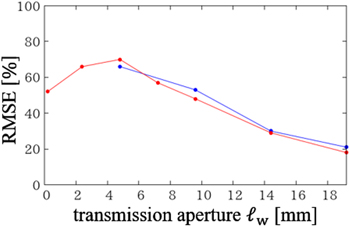
Fig. 7. (Color online) RMSE of the angular amplitude characteristics between reflection and scattering at different transmission aperture's widths  Red dots show the results of the simulation experiment. Blue dots show the results of the water tank experiment.
Download figure:
Standard image High-resolution imageFigures 8(a1) and 8(b1) show the received signals  and
and  at
at  and
and  mm for each
  th transmitted element, respectively, for
  = 4.8 mm (
 = 24). Figures 8(a2) and 8(b2) show the received signal
  at
at  and
and  mm, respectively. Figures 8(a3) and 8(b3) show the amplitudes of the received signals
  and
and  at the ideal delay times
  respectively.
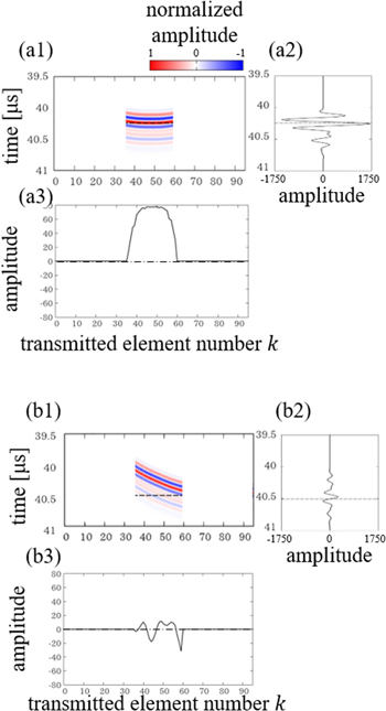
Fig. 8. (Color online) Simulation results of the reflector with a transmission aperture of 4.8 mm. The dashed lines represent the ideal delay time  (a1), (b1) Received signal
  from each transmitted element; (a2), (b2) received signals
  (a1)–(a2) results for
  mm; (b1), (b2) results for
  mm.
mm.
Download figure:
Standard image High-resolution imageThe reason for the RMSE being maximized for  = 4.8 mm (
 = 24) can be explained in two points: first, as shown in Fig. 8(a3), when
  was 4.8 mm (24 elements) or more,
  was almost the same for
  = 36–59, which accounted for a large fraction of
  at the center with regard to the received element; second, as shown in Figs. 5(a3), 5(b3), and 5(c3), the shape of
  changed as the received element position shifted. When
  = 4.8 mm (
 = 24), as shown in Fig. 8(b3), for the received element position
  apart from the center, the received signal decreased with the change in
  When
When  is larger than 4.8 mm, the number of transmitted elements with a large amplitude of
  does not decrease even if the shape of
  changes slightly; therefore, the width of the peak of
  increases, and the RMSE with the angular amplitude characteristic of scattering
  decreases. When
  is narrower than 4.8 mm, the peak of
  decreases because all the signals from the transmitted elements of
  = 36–59 have not been received. Therefore, the RMSE between
  and
and  is maximum when
  = 4.8 mm (
 = 24).
Next, we investigated the case in which the reflector was inclined to the probe surface. Figure 9 shows the angular amplitude characteristics of reflection and scattering when the reflector was tilted by 5° or 10° concerning the probe surface. The signals with large amplitude were detected with the end of the received elements  as the tilt angle increased. When the reflector was tilted by 10°, the amplitudes decreased with decreasing
  because most of the reflected signals could not be received at the receiving elements; this was because of the tilt of the reflector.

Fig. 9. Simulation results of angular amplitude characteristics of reflection for different transmission aperture's widths  (a1)–(d1) Results for a reflector tilted by 5° with respect to the probe surface; (a2)–(d2) results for a reflector tilted by 10° with respect to the probe surface; (a1), (a2) results for
  = 19.2 mm; (b1), (b2) results for
  = 14.4 mm; (c1), (c2) results for
  = 9.6 mm; (d1), (d2) results for
  = 4.8 mm.
Download figure:
Standard image High-resolution imageThe RMSEs between  and
and  for each transmission aperture's width (
 ) when the reflector was tilted by 5° or 10° to the probe surface are denoted with red and blue dots, respectively in Fig. 10. When the reflector inclination was 5°, the RMSE was maximum for
  = 4.8 mm (
 = 24). The tendency was the same as the result for the parallel reflector in Fig. 7. When the reflector was tilted by 10°, the RMSE also increased with decreasing
  although the RMSE for
  = 4.8 mm was almost the same as that for
  = 19.2 mm (
 = 96). This is because most of the reflected signals could not be received at the receiving elements for
  = 4.8 mm. Therefore, it suggests that the bone surface should be aligned as parallel as possible to the probe surface in clinical applications.
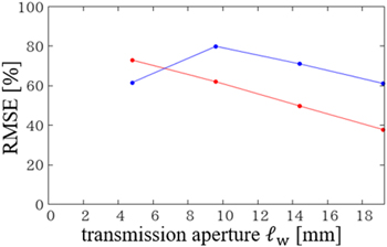
Fig. 10. (Color online) Simulation results of the RMSE of angular amplitude characteristics between reflection and scattering at different transmission aperture widths  Red and blue dots show the results for a reflector tilted by 5° and 10°, respectively.
Download figure:
Standard image High-resolution imageIn the simulation, the reflector was assumed to be flat; therefore, if the reflector was tilted to the probe surface in the elevational direction of the probe, the shape of  did not change. However, the angular amplitude characteristics from the curved surfaces such as the thoracic vertebrae would change due to phase aberration. We will investigate this effect further in our future work.
3.4. Results of the water tank experiment
Figure 11 shows  of reflection and
  of scattering for each transmission aperture's width (
 ); these were obtained from the surface of the acrylic block and the short axis of the wire, respectively, in the water tank experiment. The received signal was too weak while measuring the scatterer when
  = 0.2 mm. The results were almost similar to Fig. 6. In Fig. 7, the blue dots show the RMSE between
  and
and  for each value of
  Reflectors and scatterers can be distinguished in detail when
  = 4.8 mm.
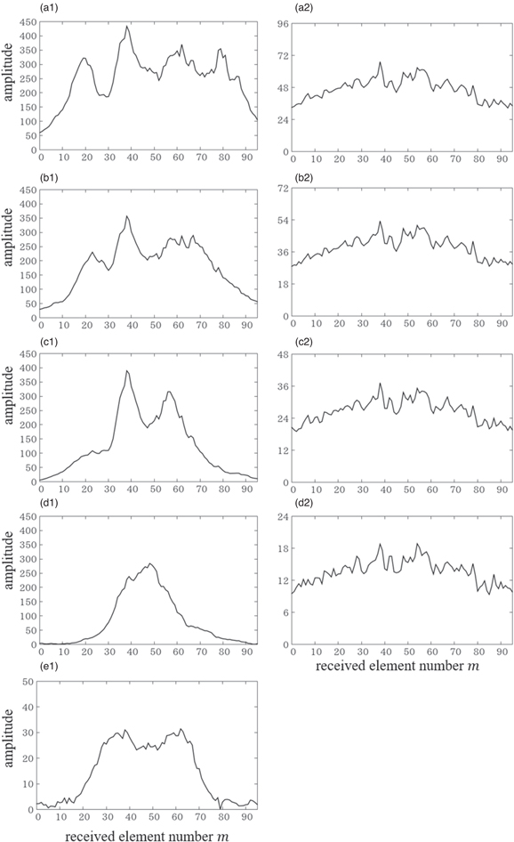
Fig. 11. Angular amplitude characteristics of reflection and scattering for the different transmission aperture  obtained from the water tank experiment. (a1)–(e1) Reflection characteristics, (a2)–(e2) scattering characteristics, (a1), (a2) results for
  = 19.2 mm; (b1), (b2) results for
  = 14.4 mm; (c1), (c2) results for
  = 9.6 mm; (d1), (d2) results for
  = 4.8 mm, (e1) results for
  = 0.2 mm. At
  = 0.2 mm, signals of the scatterer were weak and could not be detected.
Download figure:
Standard image High-resolution image3.5. Effect of the decreased transmission aperture's width on the lateral resolution
The reduction in  affects the lateral resolution of the focused wave. Figure 12(a) shows the acoustic field distribution along the lateral direction
  at a focal depth of 30 mm for each
  The horizontal axis represents the lateral position centered just above the beam. The vertical axis was normalized to the maximum amplitude for each value of
  The full-width-at-half-maximum (FWHM) increased as
  decreased.

Fig. 12. (Color online) Relationship between the transmission aperture's width  and the acoustic field distribution. (a) Acoustic field distribution along the lateral direction at a focal depth of 30 mm for each transmission aperture
  (b) Relationship between the FWHM of the transmitted beam and the RMSE of the angular amplitude characteristics of reflection and scattering at the focal depth.
Download figure:
Standard image High-resolution image
Figure 12(b) shows the relationship between the FWHM of the transmitted beam at the focal depth and RMSE of  and
and  There is a trade-off between the lateral resolution and RMSE. In thoracic spine measurements in the clinic, it is necessary to determine the appropriate transmission aperture's width
  for imaging by considering this trade-off relationship.
4. Conclusions
We investigated the ultrasound transmission conditions so that differences in the angular amplitude characteristics of reflection and scattering are emphasized more. We discussed the angular amplitude characteristics  and
and  of the reflection and scattering based on the simulation and the water tank experiment and clarified the relationship between the angular amplitude characteristics and transmission aperture's width
  For the measurement of the human thoracic vertebrae, it is necessary to consider the effect of the lateral resolution by changing
  and to investigate a suitable
  The simulation and water tank experimental results showed that the difference between
  and
and  is emphasized more, and it will significantly support thoracic epidural anesthesia in the future.
Acknowledgments
This work was partially supported by JSPS KAKENHI 20H02156.