Three-dimensional finite difference-time domain simulation of moving sound source and receiver

Among many numerical analysis methods of the sound field, the finite-difference time-domain (FDTD) method ^1–10) is one of the most commonly used tools. In most sound field analysis including the FDTD method, sound sources and receivers are usually fixed, then the responses between them are mainly calculated. However, in order to analyze the noise of automobiles ¹¹⁾ and trains, ¹²⁾ it is necessary to represent the moving sound sources in the FDTD method. In addition, the moving receiver must be also implemented for the analysis of the drone audition ^13,14) or the bat sonar mechanism. ¹⁵⁾ In the electromagnetic field analysis by the FDTD method, several studies have been conducted on the moving source by applying the Lorentz transformation. ^16,17) For the numerical analysis of moving sound sources, a method using the linearized Euler equations have been studied. ¹⁸⁾ There are some methods by which a fluid flow is analyzed instead of the sound source moving. ^19,20) In virtual reality, there are some studies on the moving sound sources for the auralization, ^21–25) but it is difficult to analyze a physically valid field since these methods cannot calculate the sound wave propagation. There are few studies on the moving receiver other than those related to the walk-through auralization. ²⁶⁾ We have already implemented a moving sound source ²⁷⁾ and a moving receiver ²⁸⁾ in the two-dimensional FDTD method directly.

In this paper, the scheme is extended to the three-dimensional compact-explicit finite-difference time-domain (CE-FDTD). ^29–35) The CE-FDTD method is a higher accuracy version of the standard FDTD method and is suitable for large scale sound field analysis. There are two methods to implement the moving sound source and receiver in the FDTD method: the direct method and the convolution method. ²⁸⁾ The direct method is only proposed in this paper to implement the moving sound source and receiver in the three-dimensional FDTD method that provides physically valid analysis including the Doppler effect. A driving method in which the grid points around the source position are driven by the source distribution function ^27,28) is proposed. While the linear distribution driving was only applied in the USE proceedings, ³⁶⁾ the Gaussian distribution driving is mainly applied in this paper. For the moving receiver, the linear interpolation method is implemented. It is assumed in this paper that the source and receiver have no boundaries. Some numerical experiments on the moving source and receiver with arbitrary trajectories are made for a three-dimensional sound field including the case where the sound source and receiver move at the same time. The accuracy of the proposed method is discussed.

The three-dimensional wave equation in the homogeneous and loss less media is given as

$$\begin{eqnarray}&&\displaystyle \frac{1}{{c}_{0}^{2}}\displaystyle \frac{{\partial }^{2}p}{\partial {t}^{2}}=\displaystyle \frac{{\partial }^{2}p}{\partial {x}^{2}}+\displaystyle \frac{{\partial }^{2}p}{\partial {y}^{2}}+\displaystyle \frac{{\partial }^{2}p}{\partial {z}^{2}},\end{eqnarray} \tag{ 1 }$$

where p is the sound pressure and c₀ is the sound speed. In the CE-FDTD method, the wave equation is directly discretized by the central finite-difference on a collocated grid where the grid intervals in the x, y and z directions is all Δ. Considering not only the axis directions but also the face diagonal and the space diagonal directions, Eq. (1) is discretized as ^31,32)

$$\begin{eqnarray}&&\begin{array}{l}{p}_{i,j,k}^{n+1}={d}_{1}\left({p}_{i+1,j,k}^{n}+{p}_{i-1,j,k}^{n}+{p}_{i,j+1,k}^{n}\right.\\ \left.+\,{p}_{i,j-1,k}^{n}+{p}_{i,j,k+1}^{n}+{p}_{i,j,k-1}^{n}\right)\\ +\,{d}_{2}\left({p}_{i+1,j+1,k}^{n}+{p}_{i+1,j-1,k}^{n}+{p}_{i+1,j,k+1}^{n}\right.\\ +\,{p}_{i+1,j,k-1}^{n}+{p}_{i,j+1,k+1}^{n}+{p}_{i,j+1,k-1}^{n}\\ +\,{p}_{i,j-1,k+1}^{n}+{p}_{i,j-1,k-1}^{n}+{p}_{i-1,j+1,k}^{n}\\ \left.+\,{p}_{i-1,j-1,k}^{n}+{p}_{i-1,j,k+1}^{n}+{p}_{i-1,j,k-1}^{n}\right)\\ +\,{d}_{3}\left({p}_{i+1,j+1,k+1}^{n}+{p}_{i+1,j-1,k+1}^{n}\right.\\ +\,{p}_{i+1,j+1,k-1}^{n}+{p}_{i+1,j-1,k-1}^{n}\\ +\,{p}_{i-1,j+1,k+1}^{n}+{p}_{i-1,j-1,k+1}^{n}+{p}_{i-1,j+1,k-1}^{n}\\ \left.+\,{p}_{i-1,j-1,k-1}^{n}\right)+{d}_{4}{p}_{i,j,k}^{n}-{p}_{i,j,k}^{n-1},\end{array}\end{eqnarray} \tag{ 2 }$$

where ${p}_{i,j,k}^{n}$ represents the sound pressure on the grid point (x, y, z) = (iΔ, jΔ, kΔ) at time t = nΔt, and Δt is the time step, χ = c₀Δt/Δ is the Courant number. ³⁷⁾ The coefficients d₁–d₄ are given by

$$\begin{eqnarray}&&\begin{array}{l}{d}_{1}={\chi }^{2}(1-4a+4b),{d}_{2}={\chi }^{2}(a-2b),{d}_{3}={\chi }^{2}b,\\ {d}_{4}=2(1-3{\chi }^{2}+6a{\chi }^{2}-4b{\chi }^{2}),\end{array}\end{eqnarray} \tag{ 3 }$$

where a and b are the parameters to control numerical accuracy. In this paper, a = 1/4 and b = 1/16 are used as the interpolated wide-band (IWB) scheme. The sound field analysis tool based on the CE-FDTD method has already been well verified in previous researches. ^32–35)

2.1. Implementation of moving sound source and receiver

First, a moving sound source is considered. In order to implement a moving sound source in the FDTD method, it is necessary to switch and drive the grid points on the moving path of the source. When the point source is just on the grid point, it is sufficient to drive the grid point. However, when the sound source is located between the grid points, it is necessary to distribute and drive the sound source to the adjacent grid points. In the previous two-dimensional case, ^27,28) some artifacts were confirmed in the calculation results only for the moving source when the adjacent grid points were driven. In order to reduce the artifacts, another driving method is proposed in this paper in which the grid points around the source position are driven with the source distribution function. Two types of the source distribution driving are considered: the linear distribution driving and the Gaussian distribution driving ³⁸⁾ which is one of the smooth distributions.

For the linear distribution driving, the grid points (i, j, k) near the source position are driven by the following function.

$$\begin{eqnarray}&&{f}_{s}^{n}(i,j,k)=(1-\alpha {d}_{s})U(1-\alpha {d}_{s}),\end{eqnarray} \tag{ 4 }$$

where d_s is the distance between the center of the source position $({x}_{s}^{n},{y}_{s}^{n},{z}_{s}^{n})$ at the time t = nΔt and the grid point (i, j, k), U is the unit step function, and α is the parameter to control the sound source size. For the Gaussian distribution driving, the grid points are driven by the following function.

$$\begin{eqnarray}&&{f}_{s}^{n}(i,j,k)={e}^{-\alpha {d}_{s}^{2}}.\end{eqnarray} \tag{ 5 }$$

In both cases, the grid points within 2Δ of the distance from the sound source are simultaneously driven with the amplitude of fⁿ (i, j, k)sⁿ where sⁿ is the sound source signal at t = nΔt.

Next, a moving sound receiver is implemented. In the case of a moving sound receiver, a simple interpolation is implemented since it has been found that no artifacts are confirmed by the numerical experiments in two dimensions. ²⁸⁾ It is assumed that the receiver is located at $({x}_{r}^{n},{y}_{r}^{n},{z}_{r}^{n})=({x}_{i}^{n}+{d}_{x}^{n},{y}_{j}^{n}+{d}_{y}^{n},{z}_{k}^{n}+{d}_{z}^{n})$ between eight grid points P₁–P₈ at the time t = nΔt as shown in Fig. 1 (a), where $0\leqslant {d}_{x,y,z}^{n}\leqslant {\rm{\Delta }}$. In the moving receiver, the local coordinate system (ξ, η, ζ) is introduced as shown in Fig. 1 (b). On the local coordinate, the sound source position is converted to $({\xi }_{i}^{n},{\eta }_{j}^{n},{\zeta }_{k}^{n})$ where −1 ≤ ξ, η, ζ ≤ 1. The sound pressure at the receiver is interpolated from the sound pressures of the adjacent eight grid points as

$$\begin{eqnarray}&&{p}^{n}=\sum _{i=1}^{8}{w}_{i}^{n}{p}_{i}^{n},\end{eqnarray} \tag{ 6 }$$

where p_i ⁿ and w_i ⁿ are the sound pressure and the interpolation function at the grid point P_i , respectively ^27,28)

$$\begin{eqnarray}\begin{array}{rcl}{w}_{1}^{n} & = & (1-{\xi }_{i}^{n})(1-{\eta }_{j}^{n})(1-{\zeta }_{j}^{n})/8,\\ {w}_{5}^{n} & = & (1-{\xi }_{i}^{n})(1-{\eta }_{j}^{n})(1+{\zeta }_{j}^{n})/8,\\ {w}_{2}^{n} & = & (1+{\xi }_{i}^{n})(1-{\eta }_{j}^{n})(1-{\zeta }_{j}^{n})/8,\\ {w}_{6}^{n} & = & (1+{\xi }_{i}^{n})(1-{\eta }_{j}^{n})(1+{\zeta }_{j}^{n})/8,\\ {w}_{3}^{n} & = & (1+{\xi }_{i}^{n})(1+{\eta }_{j}^{n})(1-{\zeta }_{j}^{n})/8,\\ {w}_{7}^{n} & = & (1+{\xi }_{i}^{n})(1+{\eta }_{j}^{n})(1+{\zeta }_{j}^{n})/8,\\ {w}_{4}^{n} & = & (1-{\xi }_{i}^{n})(1+{\eta }_{j}^{n})(1-{\zeta }_{j}^{n})/8,\\ {w}_{8}^{n} & = & (1-{\xi }_{i}^{n})(1+{\eta }_{j}^{n})(1+{\zeta }_{j}^{n})/8,\end{array}\end{eqnarray} \tag{ 7 }$$

where ${\xi }_{i}^{n}=2{d}_{x}^{n}/{\rm{\Delta }}-1,{\eta }_{j}^{n}=2{d}_{y}^{n}/{\rm{\Delta }}-1,{\zeta }_{k}^{n}=2{d}_{z}^{n}/{\rm{\Delta }}-1$ are the local coordinates normalized by the grid interval Δ. This receiving method corresponds to an array receiver with eight receivers distributed in a single cell.

Zoom In Zoom Out Reset image size

2.2. Doppler shift

As shown in Fig. 2, it is assumed that a sound source moves with a velocity v _S and a receiver moves with a velocity v _R. The Doppler shift is determined by the radial velocity, which is the velocity along the line between the source and receiver. The position and the radial velocity of the sound source are evaluated at the time t_S when the sound wave is radiated, and that of the receiver is evaluated at the time t_R when the sound wave is received. The magnitude of the radial velocity v_SR for the sound source and the radial velocity v_RS for the receiver are, respectively, given as

$$\begin{eqnarray}&&{v}_{\mathrm{SR}}=\displaystyle \frac{({{\boldsymbol{r}}}_{{\rm{R}}}({t}_{{\rm{R}}})-{{\boldsymbol{r}}}_{{\rm{S}}}({t}_{{\rm{S}}}))\cdot {{\boldsymbol{v}}}_{{\rm{S}}}({t}_{{\rm{S}}})}{| {{\boldsymbol{r}}}_{{\rm{R}}}({t}_{{\rm{R}}})-{{\boldsymbol{r}}}_{{\rm{S}}}({t}_{{\rm{S}}})| }\ ,\end{eqnarray} \tag{ 8 }$$

$$\begin{eqnarray}&&{v}_{\mathrm{RS}}=\displaystyle \frac{({{\boldsymbol{r}}}_{{\rm{R}}}({t}_{{\rm{R}}})-{{\boldsymbol{r}}}_{{\rm{S}}}({t}_{{\rm{S}}}))\cdot {{\boldsymbol{v}}}_{{\rm{R}}}({t}_{{\rm{R}}})}{| {{\boldsymbol{r}}}_{{\rm{R}}}({t}_{{\rm{R}}})-{{\boldsymbol{r}}}_{{\rm{S}}}({t}_{{\rm{S}}})| }\ ,\end{eqnarray} \tag{ 9 }$$

where r _S and r _R denote the position vectors of the receiver and the source, respectively. So the normalized Doppler shift D at the receiver R is given as

$$\begin{eqnarray}&&D=\displaystyle \frac{{f}_{{\rm{R}}}}{{f}_{{\rm{S}}}}=\displaystyle \frac{{c}_{0}-{v}_{\mathrm{RS}}}{{c}_{0}-{v}_{\mathrm{SR}}},\end{eqnarray} \tag{ 10 }$$

where f_R is the receiving frequency, and f_S is the radiated source frequency.

Zoom In Zoom Out Reset image size

First, we consider the case where the trajectory of the sound source and receiver is linear. Figure 3 shows the 3D numerical model for the sound source or receiver moving on a linear trajectory. A cubic region of 21 × 21 × 21 m³ is assumed and divided into FDTD cells of 1400 × 1400 × 1400, so the grid size is Δ = 15 mm. The time step is Δt = 43.68 μs, and the sound speed is c₀ = 340 m s⁻¹, so the Courant number χ is 0.99. In the case of the moving source, the source P moves linearly from the center of the region in the direction of horizontal angle ϕ and elevation angle θ at a constant speed v. The fixed receivers Q₁ and Q₂ are placed at a distance of 10 m from the sound source. In the case of the moving receivers, point P is a moving receiver and the point Q₁ or Q₂ is a fixed source that radiates sound waves only from one or the other. The direction from point P to point Q₁ is assumed to be positive. The boundary condition is Mur's first-order absorbing boundary. ³⁹⁾ The calculations were performed in single precision on a graphics processing unit (NVIDIA Quadro RTX 8000) machine.

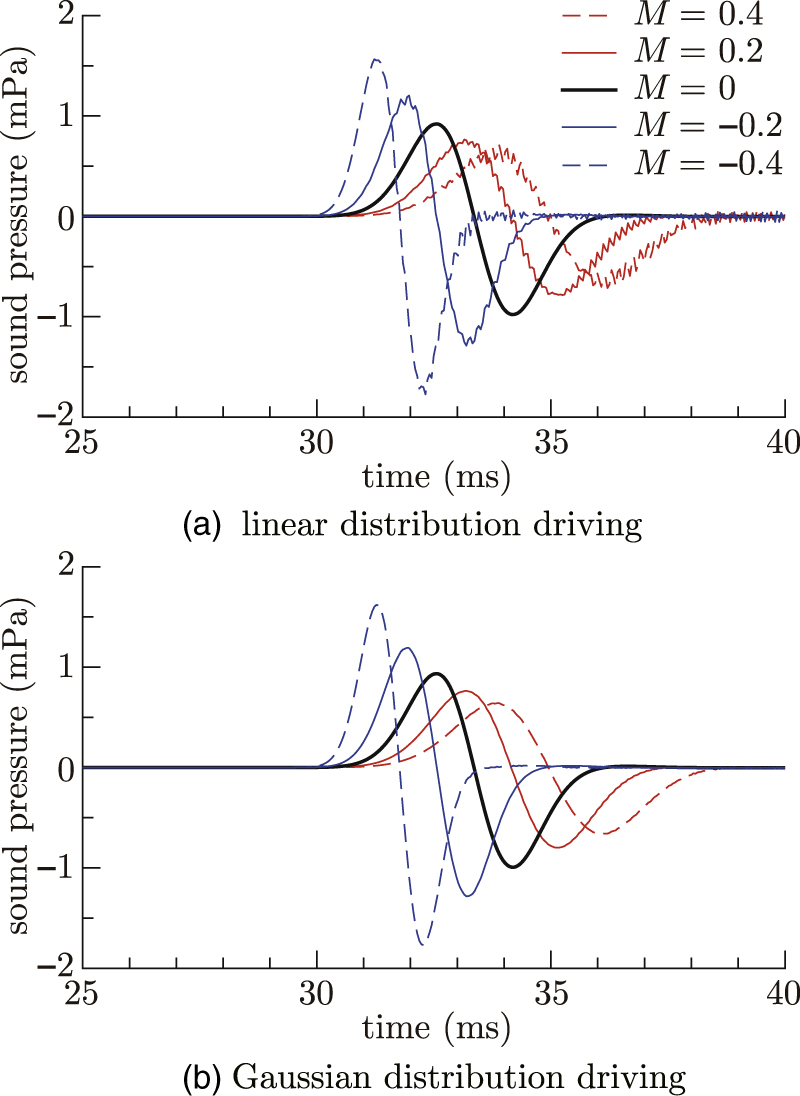
Zoom In Zoom Out Reset image size

Figure 4 shows the sound pressure waveforms calculated at the receiver for the moving source. The source moves with a constant speed of v = 64 m s⁻¹ (Mach number M = 0.2), v = 128 m s⁻¹ (M = 0.4) in the direction of θ = 0, ϕ = 0. A differential Gaussian pulse with a pulse width of 6 ms is radiated from the source at the time t = 0 s. The velocity at which point P moves toward point Q₁ is assumed to be positive. Figure (a) shows the results for the linear distribution driving with α = 0.29 and (b) shows the Gaussian distribution driving with α = 46.67. It is shown that the waveform is compressed in the moving direction of the source and is expanded in the opposite direction due to the Doppler effect. However, strong artifacts can be confirmed in the waveform calculated by the linear distribution driving, while there are no artifacts for the Gaussian distribution driving. The artifact was also observed in the two-dimensional case ²⁸⁾ and is due to the driving method of the sound source from the present numerical experiments. It is found that the source distribution should be smooth such as a Gaussian shape. In all subsequent numerical experiments, the calculations are performed using the Gaussian distribution driving.

Zoom In Zoom Out Reset image size

Figure 5 shows the sound pressure waveforms calculated at the receiver for the moving receiver. The Doppler effect can be confirmed as with the moving sound source, and no artifacts can be confirmed for the moving receiver. It is confirmed that the proposed method can simulate the moving sound source or receiver with the Doppler effect.

Zoom In Zoom Out Reset image size

Figure 6 shows the normalized Doppler shift against the Mach number M for θ = 0, ϕ = 0. A continuous sine wave with a frequency of 500 Hz is radiated from the source. Figure (a) shows the results for the moving source and (b) shows the moving receiver. The Doppler shift is calculated by analyzing the sound pressure waveform calculated at the receiver using the fast Fourier transformation. The calculated Doppler shift by the FDTD method agrees well with the theoretical value.

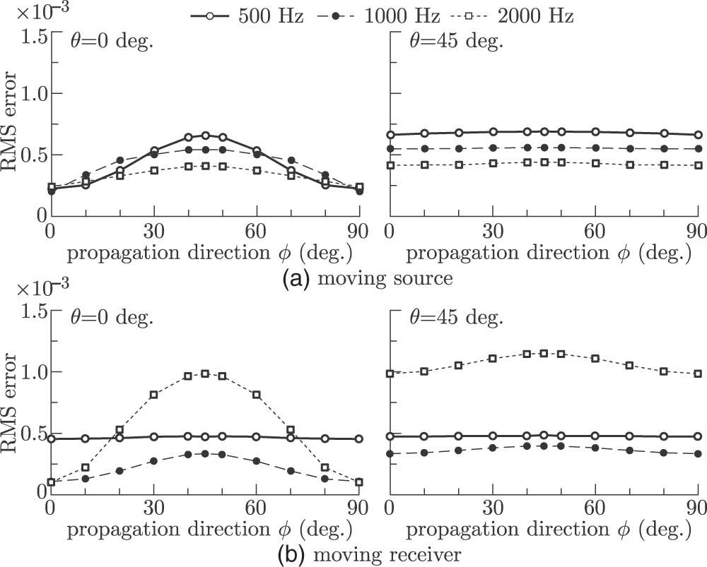
Zoom In Zoom Out Reset image size

The accuracy is evaluated by the root mean square (RMS) error between the calculated and the theoretical values of the normalized Doppler shift, which is expressed by the following equation:

$$\begin{eqnarray}&&\varepsilon =\sqrt{\displaystyle \frac{1}{N}\sum _{i=1}^{N}{\left({d}_{i}-{D}_{i}\right)}^{2}},\end{eqnarray} \tag{ 11 }$$

where N is the number of the evaluation samples, d_i is the normalized Doppler shift calculated by the FDTD method, and D_i is the theoretical one calculated by Eq. (10). Figure 7 shows the root mean square error of the normalized Doppler shift against the traveling direction ϕ with a frequency of 500 Hz (45.3 points per wavelength), 1000 Hz (22.7 p. p. w.), and 2000 Hz (11.3 p. p. w.) for the range of source speed M = −0.5 to 0.5. In both cases, the RMS error shows a symmetrical characteristic around 45 degrees, which is a reasonable result on an equally spaced collocated grid in the FDTD calculation. Figure 8 shows the root mean square error against the source frequency for ϕ = 0. In both cases, the RMS error becomes large as the frequency increases except for the low frequency where the frequency estimation performance decreases. The error is within 1.5 × 10⁻³ in all directions and frequencies. Since the threshold of the human frequency discrimination is about 0.2%, ⁴⁰⁾ the RMS error is comparable to this criterion. It is confirmed that the moving sound source and receiver can be calculated accurately by the present method.

Zoom In Zoom Out Reset image size

Zoom In Zoom Out Reset image size

A moving sound source or receiver passing linearly in front of the receiver or source is next demonstrated. Figure 9 shows the numerical model for the linearly passing source or receiver. The sound source or receiver P passes linearly 2 m in front of the receiver or source with an initial speed of M = 0.1 and an acceleration of a = 0, 60 m s⁻². The source radiates a continuous sine wave with a frequency of 500 Hz. Figure 10 shows the normalized Doppler shift calculated by the short-time Fourier transform of the sound pressure waveform calculated at the receiver. In the figure, the center frequency of the power spectrum is estimated by the reassignment method ⁴¹⁾ in MATLAB toolbox. The reassignment method is a technique to sharpen the time-frequency representation by mapping the data to time-frequency coordinates closer to the true support region of the analyzed signal. In both cases, the Doppler shift from high to low frequencies is well reproduced as the source or receiver passes. The calculated result and the theoretical result show good agreement even in the case of acceleration.

Zoom In Zoom Out Reset image size

Zoom In Zoom Out Reset image size

Figure 11 shows the root mean square error of the normalized Doppler shift against the traveling direction θ for various source frequencies. For the evaluation points estimated by the reassignment method, the RMS error is calculated using Eq. (11). The RMS error is asymmetrical about the angle since the number of the evaluation points N = 250–285 is different for each calculation in the reassignment method. Both the moving sound source and receiver have the almost same RMS error. In all cases, the RMS error for the constant velocity moving is smaller than that for the accelerated moving. The RMS error is within 0.7 × 10⁻³ for the constant speed, and 1.4 × 10⁻³ for the acceleration in all directions and frequencies. It is found that the moving source and receiver can be simulated even when the Doppler frequency changes continuously.

Zoom In Zoom Out Reset image size

Finally, we examined the case when the sound source and receiver move at the same time. Figure 12 shows the case when the sound source S and receiver R move on the linear trajectory facing each other. Figure (a) shows the numerical model and (b) shows the normalized Doppler shift. The initial velocity of both the sound source and receiver is M = 0.1 and the acceleration is a = 0, 60 m s⁻². They move linearly over a distance of 20 m with an interval of 2 m. A continuous sine wave with a frequency of 500 Hz is radiated from the source. The calculated results and the theory are in good agreement. Table I shows the RMS error. The RMS error becomes large in the case of the diagonal moving or the accelerated moving.

Zoom In Zoom Out Reset image size

The case when a source–receiver pair moves on a circular trajectory is lastly examined. It is assumed that the sound source S and the receiver R are separated by 2 m, and their center of gravity moves in a circular trajectory with a radius of 8 m as shown in Fig. 13 (a). So, the source and receiver move with the same angular velocity keeping the distance at 2 m. The velocity of the center of gravity is M = 0.1 or the angular velocity is 2.267 rad s⁻¹. To extract only the reflected wave, the sound pressure waveform without the reflecting wall is also calculated, then the direct wave is removed by subtracting it from the waveform with the reflecting wall. Figure (b) shows the normalized Doppler shift. The Doppler shift changes sinusoidally. When the orbit is tilted (θ = 45°), the reflection angle on the wall becomes smaller, so the Doppler shift becomes smaller. It is confirmed that the proposed method can be applied even when the sound source and receiver move in an arbitrary trajectory at the same time.

Zoom In Zoom Out Reset image size

Moving sound source and receiver with arbitrary trajectories were implemented in the three-dimensional CE-FDTD method. Two types of source distribution driving were proposed for the moving sound source: the linear distribution driving and the Gaussian distribution driving that achieves smooth distribution. It is found that the artifacts can be confirmed in the waveform calculated by the linear distribution driving, while there is no artifact for the Gaussian distribution driving. It is confirmed that the Gaussian distribution driving is suitable for the analysis of the moving sound sources. For a moving receiver, the sound pressure at the receiver was interpolated from the sound pressures of the adjacent eight grid points. As the results of the three-dimensional numerical experiments, it is confirmed that the proposed method can be applied to the moving sound source and receiver including the Doppler effect.