
Abstract
The objective of this study is to achieve vehicle self-localization using a single acoustic ranging sensor in a multipath environment. For this purpose, we proposed a measurement method of multiple time-of-flight (ToF) using an acoustic ranging sensor and a self-localization method using the ToFs. The proposed method predicts the ToFs based on the wall position and the predicted self-location and corrects the self-location by comparing it with the actual ToFs. Sound waves radiated indoors are reflected multiple times by every wall, ceiling, and floor. Therefore, the observed signal contains multiple reflected waves. Since the conventional method only considers a single reflection, self-localization becomes challenging in a multiple reflection environment. We showed that the estimation accuracy can be improved by utilizing the multiple reflections of sound waves in three-dimensional space and modeling them. The experiments confirm that the average location error of the proposed method is 0.084 m.
Export citation and abstract BibTeX RIS
1. Introduction
Vehicle navigation technology has been used widely in the automation of construction sites and factories. Developers combine various elements such as self-localization, obstacle detection, and path planning to achieve vehicle navigation. Among these elements, the self-localization technique strongly determines the accuracy of robot navigation. Generally, developers use the global navigation satellite system (GNSS) for self-positioning outdoors. 1) However, GNSS cannot be used indoors where satellite signals cannot reach. Instead, developers use a self-positioning method employing bluetooth low energy (BLE) and Wi-fi as beacons. 2) They use the intensity distribution of radio waves emitted from multiple beacons as a map and compare it with the measured radio wave intensity to achieve self-positioning. Methods utilizing beacons have also been proposed, such as those using the direction of arrival of sound waves and infrared light. 3–11) These methods are not suitable for self-positioning estimation in large spaces because the number of beacons that must be installed increases as the moving area increases. Therefore, a solution without using beacons has also been proposed. This is a method uses a sensor mounted on the vehicle to measure the wall surface and estimate its position. Light detection and ranging (LiDAR) and ultrasonic sensors are typically employed. LiDAR acquires the distance of the surroundings by scanning a laser with a mirror. The vehicle can estimate its position by matching the point cloud obtained from the sensor with the information on the map and can estimate self-position with high accuracy. 12–14) However, LiDAR cannot detect a transparent object it is not robust against optical scatterers. Ultrasonic sensors measure distance by measuring the time it takes for the sound to reach the receiver from the transmitter. 15–19) Various time-of-flight (ToF) measurement methods have been proposed by applying digital communication technology. 20–27) Numerical methods for moving sources have also been proposed for the design of sensors and measurement algorithms. 28) A method using ultrasonic sensors can detect transparent objects and is not much affected by optical scatterers. However, ultrasound is not suitable for large space applications due to its high attenuation in the air. The method using parametric speakers enables high resolution and long-range sensing, but it does not provide omnidirectional information. 16,17) Multiple transmitters and receivers need to be placed on the vehicle to acquire the distance in all directions. Therefore, a method to obtain omnidirectional distance using only a loudspeaker and a microphone was proposed. 29) A sensor emits sound in all directions and measures the ToF of the reflected waves from all around. From the response waveform, the reflected wave arriving from all directions are detected, and the arrival times of the reflected wave are measured. However, since the arrival direction of the reflected wave is unknown, the location of the reflection point cannot be determined. A self-positioning method using such a distance measurement by a single sound source has been proposed and verified by simulation. 30,31) However, there have been no reports of successful self-localization using this method in experiments. We propose a signal processing method and a self-localization method using a single acoustic ranging sensor, and we show that the self-localization method is successful in indoor environments.
For self-localization using conventional methods, the complex acoustic multipath in indoor environments is a challenge. 32) Although conventional methods focus only on the first reflection peak, multi-reflection peaks such as corner reflections exist in the actual reflection pattern. In addition, conventional methods consider only reflected waves on a two-dimensional plane, whereas in reality the sound radiates in three dimensions and is reflected by ceilings and floors as well as walls. Numerical methods have been proposed to overcome the complex multipath and Doppler effects of moving sources. However, real-time operation using numerical methods is impractical. We have proposed a self-localization method based on a Kalman filter with a map, using the commands to the vehicle's wheels and the sensor values acquired by the acoustic ranging sensor as inputs. The study showed that the use of multipath in 3D space in the observation model for the Kalman filter can improve the accuracy of the estimation. 33) However, we found that initial horizontal angle error increases the position estimation error when using the method in Ref. 33. Therefore, the purpose of this paper is to develop and propose a self-localization method robust to initial horizontal angle error by considering the existence of undetected reflected waves during ToF detection.
This paper is composed of five sections. Section 2 describes the proposed method. Section 3 describes the experimental environment. Section 4 describes the results and discussion. Section 5 concludes the paper.
2. Proposed method
2.1. Measurement of multiple ToFs using acoustic ranging sensors
We propose a signal processing method to measure multiple ToFs using a single pair of acoustic transmitters and receivers. The acoustic ranging sensor consists of a time-synchronized loudspeaker and a microphone, which is placed on top of it. Figure 1 shows an overview of signal processing. ToFs are measured by using the pulse compression technique with an M-sequence signal as the transmission signal. The transmitted signal is a sinusoidal wave with a carrier frequency of fc phase modulated by an M-sequence signal of sequence length L. One symbol of the M-sequence signal and one period of the carrier signal have the same time interval, and the signal length of one sequence is L(fs/fc) when the sampling frequency is fs. The received signal ri(k) is a signal block of length 2L(fs/fc) cut out from a continuously recorded signal. The transmitted signal si(k) is a signal block cut out from the drive signal of the loudspeaker for the same length at a timing synchronized with the received signal ri(k). The received signal is bandlimited by a bandpass filter with a low cutoff frequency flow and a high cutoff frequency fhigh. The circular cross-correlation operation is performed on the transmitted and received signals to calculate the impulse response. The circular cross-correlation operation is
where hi(k) is the impulse response between the loudspeaker and the microphone measured after the elapse of iΔt seconds. The path of sound propagation from the loudspeaker to the microphone includes direct and reflected waves. When the sensor is in motion, the reflected wave always changes depending on its position relative to the wall. On the other hand, the direct wave always has the same response. Therefore, the background subtraction operation between waveforms can eliminate the direct wave. The background subtraction operation is

where Na is the window length of the moving average. Peak detection into the envelope of the signal  extracts the ToFs. The envelope of the signal is represented by

where  is the Hilbert transform of a discrete-time signal. The peak detector set the minimum peak height ph, the minimum peak width pw, and the detection range
  , and detected the local maximum value that satisfied the conditions. The minimum peak height ph is set as a percentage of root mean square of h1(k). The peak width was measured by using the peak prominence implemented in Matlab2020a. The ToF of the #j reflected wave detected in the #i measurement is

where  is the index of the #j peak detected in the #i measurement.

Fig. 1. (Color online) Signal processing of acoustic ranging sensor.
Download figure:
Standard image High-resolution image2.2. Self-localization using a three-dimensional acoustic time-of-flight estimation model
The self-localization method (Fig. 2) uses the ToFs obtained from the acoustic ranging sensor and the commands input to the vehicle's wheels. The vehicle has two drive wheels and operates by commanding a straight-line velocity v and a turning angular velocity ω. Process (1) uses the kinematic model of the vehicle to predict the position after one step α i∣i−1. The kinematic model of the vehicle is


where
α
i−1∣i−1 is the value of the
α
estimated in the #i − 1 step, x and y are the vehicle's position in the two-dimensional plane and ϕ is the vehicle's angle. Process (2) predicts the ToFs of the reflected wave after one step. The ray acoustics theory in 3D space gives all the reflection paths of an omnidirectional sound wave emitted from the loudspeaker location until it reaches the microphone location. The equation of the plane aj
x + bj
y + cj
z + dj
= 0 is given in advance as the map information as shown in Fig. 3. The location of the mirror image of source ![${\boldsymbol{P}}({\boldsymbol{\alpha }})\,={\left[x\ y\ z\ 1\right]}^{{\rm{T}}}={\left[{\alpha }^{(1)}\ {\alpha }^{(2)}\ z\ 1\right]}^{{\rm{T}}}$](https://content.cld.iop.org/journals/1347-4065/61/SG/SG1037/revision2/jjapac506cieqn5.gif) due to the effect of wall #j is
due to the effect of wall #j is

where ηj
is  . The length of the reflection path is the distance between the source
P
(
α
) and the mirror image source
. The length of the reflection path is the distance between the source
P
(
α
) and the mirror image source  . Therefore, the ToF of the reflected wave for wall #j is

where I is the unit matrix and ca is the speed of sound. In the case where the reflected wave passes through two walls #j1 and #j2, the ToF of the reflected wave is

When a reflected wave passes through two walls, it never passes through the same wall twice. Therefore, the condition of Eq. (11) is j1 ≠ j2. All combinations of Eqs. (10) and (11) are enumerated as


where M is the number of walls and m is an integer of 1 ≤ m ≤ M2.  is the predicted value of ToFs when moving to location
α
i∣i−1. Process (3) measures the actual arrival ToFs using an acoustic ranging sensor. Process (4) calculates the error between the predicted and measured ToFs using equation
is the predicted value of ToFs when moving to location
α
i∣i−1. Process (3) measures the actual arrival ToFs using an acoustic ranging sensor. Process (4) calculates the error between the predicted and measured ToFs using equation


where  is
is  . Estimation of the self-localization is done by

where K i is the Kalman gain. The Kalman gain is based on the extended Kalman filter algorithm to determine the optimal gain. The prediction function of the ToFs after comparison with the actual ToFs is

where Qi is the number of ToFs measured. The Jacobians of the vehicle's kinematic model function f ( α , u ) and ToF prediction function γ i ( α ) are


We assume that the errors in the prediction of the location by the function f ( α , u ) and the prediction of the ToF by the function γ i ( α ) follow a normal distribution, and their variance-covariance matrices are E i and W i . The Kalman gain is calculated by sequentially computing Eqs. (22)–(25)


Ψi∣i−1 is the prior prediction error covariance matrix and Ψi∣i is the posterior estimation error covariance matrix.

Fig. 2. (Color online) Self-localization process.
Download figure:
Standard image High-resolution image
Fig. 3. Reflection paths of sound waves radiated in 3D space.
Download figure:
Standard image High-resolution image3. Experimental setup
Figure 4 shows the vehicle used in the experiment. The acoustic ranging sensor, located on the top of the vehicle(iRobot Create; iRobot), consists of a loudspeaker (LSPX-S2; Sony) and a microphone (WM-61A; Panasonic). An infrared marker was attached to the top of the vehicle to obtain the reference position. Figure 5 shows the directional characteristics of this loudspeaker and microphone. The A-D/D-A converter (NI-6212; National Instruments) performs analog conversion of the transmitted signal generated by the PC and digital conversion of the signal received by the microphone. Table I shows the signal processing parameters. Figure 6 shows the experimental environment. The material of Wall1, Wall2, Wall3 and the floor is concrete. The material of the ceiling is plasterboard. The material of Wall4 is plastic. Different walls are made of different materials, but their effect is negligible. Since the plastic plate is thin compared to the wavelength, it is modeled as a mass load. Its acoustic impedance Zp is Zp = j2π f ρs, where ρs is the face density of the plastic plate. 34) The plastic plate used in this experiment has ρs = 0.50 kg m−2. When a thin plastic plate reflects sound waves propagating in the air, the energy reflectance is

where Za denotes the acoustic impedance of air, where Za is set to 400 Ns m−3. Calculating Eq. (26), the reflectance of the energy from the plastic plate is RE = 0.99 at 10 kHz, RE = 0.94 at 1 kHz, and RE = 0.13 at 100 Hz. Although the reflected energy becomes smaller at lower frequencies, it is close to total reflection in the frequency range of 2–18 kHz, which is the frequency range used in this experiment. Table II shows the map in Fig. 6 transformed into the parameters of the plane equation. A motion capture system (OptiTrack Prime13x; OptiTrack) consisting of two infrared cameras acquires the vehicle's reference position. Figure 7 shows the velocity command values for the vehicle. Figure 8 shows the predictive models of the acoustic reflection path used for self-localization: (i) a model of single reflection, (ii) a model of single and double reflections in a two-dimensional plane, (iii) a model of single and double reflections in three-dimensional space, and (iv) a model of single and double reflections in dynamically changing three-dimensional space.

Fig. 4. (Color online) Vehicle used in the experiment. (1) is a vehicle (iRobot Create; iRobot), (2) is a loudspeaker (LSPX-S2; Sony). (3) is a microphone (WM-61A; Panasonic). (4) are infrared markers for motion capture systems.
Download figure:
Standard image High-resolution image
Fig. 5. (Color online) Directional characteristics of speakers and microphones.
Download figure:
Standard image High-resolution image
Fig. 6. Experimental environment. The material of Wall1, Wall2, Wall3 and the floor is concrete. The material of the ceiling is plasterboard. The material of Wall4 is plastic.
Download figure:
Standard image High-resolution image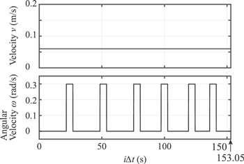
Fig. 7. Velocity command values for the vehicle.
Download figure:
Standard image High-resolution image
Fig. 8. Example of a reflection path considered by an acoustic reflection models. (i) A model of single reflection, (ii) a model of single and double reflections in a two-dimensional plane, (iii) a model of single and double reflections in three-dimensional space, and (iv) a model of single and double reflections in dynamically changing three-dimensional space.
Download figure:
Standard image High-resolution imageTable I. Signal processing parameters.
| Carrier frequency | fc | 10 kHz |
| Sequence length | L | 1023 |
| Sampling frequency | fs | 40 kHz |
| Low cutoff frequency | flow | 2 kHz |
| High cutoff frequency | fhigh | 18 kHz |
| Interval for impulse response calculation | Δt | 0.05 s |
| Window length of background subtraction | Na | 5 |
| Window length of moving average | Nb | 50 |
| Min peak height | ph | 8.5% |
| Min peak width | pw | 0.75 ms |
| Detection range |

| 0.083 s |
Table II. Parameters of the plane equation (aj x + bj y + cj z + dj = 0).
| j | aj | bj | cj | dj |
|---|---|---|---|---|
| 1 (Wall1) | 1.00 | 0 | 0 | 0 |
| 2 (Wall2) | 0 | 1.00 | 0 | 0 |
| 3 (Wall3) | 1.00 | 0 | 0 | −3.00 |
| 4 (Wall4) | 0 | 1.00 | 0 | −3.50 |
| 5 (Floor) | 0 | 0 | 1.00 | 0 |
| 6 (Ceiling) | 0 | 0 | 1.00 | −2.60 |
4. Results and discussion
Figure 9(a) shows  , where the background subtraction operation is applied to the impulse response waveform. The horizontal axis is the time axis of the impulse response at each measurement point. The vertical axis is the time elapsed since the vehicle started its operation. Figure 9(d) shows the waveform 100 s after the vehicle starts its motion. Since the background difference operation removes the values that do not vary, the reflected wave can be observed without being hidden by the direct wave. Figures 9(b) and 9(e) show the envelope
  of Figs. 9(a) and 9(d), respectively. The white area of Fig. 9(b) shows the reflected wave. Figures 9(c) and 9(f) show the detection of multiple ToFs from Figs. 9(b) and 9(e), respectively. The solid blue and red lines are the true value of ToFs, and the black dots are observed ToF values. The true value of ToF was calculated from the self-location observed by the motion capture system and the location of the wall. Figure 9(c) shows that the ToF varies continuously with vehicle movement, indicating that the relative distances between the vehicle and the wall vary as the vehicle moves. Comparison of the observed values with the true values in Fig. 9(c) reveals that the distribution of observed values is near the true values. On the other hand, some reflected waves are not detected or are detected at the wrong time. In particular, at around 5 ms, the true value shows a double line. In some cases, however, only one of the lines appears in the observed results. Of the two true lines, the fastest ToF was a reflected wave from the nearest wall, and the other ToF was a double reflected wave through the nearest wall and floor. This indicates that there are reflected waves not only from the wall surface but also from the corners composed of the wall and ceiling or the wall and floor. Figure 5 shows that the loudspeaker radiates sound strongly in any direction from −45° to 90°. It also radiates strongly in the diagonal upward and diagonal downward directions. The sound waves radiated diagonally downward are reflected at the corner composed of the wall and the floor and interfere with the reflected waves from the wall. The interference of these two reflected waves significantly degraded the detection accuracy of one of them. Therefore, double reflections (e.g. corner reflections) also significantly affect the impulse response waveform. In addition, ToFs that do not vary with vehicle motion (e.g. reflections only from the floor or ceiling and double reflections from two parallel walls) are not detected. The reason for this is that background subtraction is applied to remove the direct-current waves.

Fig. 9. (Color online) ToF detection results by acoustic ranging sensor. (a) Impulse response  applying the background difference operation. (b) Envelope of
  . (c) Observed and true values of ToFs. (d) (e) Waveforms of (a) and (b) at 100 s after the vehicle starts moving. (f) Detection timing of ToFs at 100 s after the vehicle starts moving. ToFs are detected at the timing when the detection event is set to 1.
Download figure:
Standard image High-resolution imageFigure 10 shows the self-localization results using four models: (i) the model of single reflection, (ii) the model of single and double reflections in a two-dimensional plane, (iii) the model of single and double reflections in three-dimensional space, and (iv) the model of single and double reflections in dynamically changing three-dimensional space. The estimation results using (i) deviated significantly from the true value, and the trajectory changed in the middle of the estimation in a direction different from the true value. The estimation results using (ii), (iii), and (iv) are close to the true value. Figure 11 shows the distribution of the location error for each method. The location error is the Euclidean distance between the estimated location and the true location. Method (iv) had the highest accuracy, with an average location error of 0.084 m. In cases (i) and (ii), the model does not include double reflections by the floor and walls. If the system detects a ToF due to such a reflection path, it will compare it with a ToF due to a different reflection path. In this situation, the Kalman filter will not estimate correctly because the predicted ToF does not properly match the observed ToF. Therefore, we considered that methods (iii) and (iv) improved accuracy through the increase in the number of correctly matched ToFs by including more reflection paths in the model.

Fig. 10. (Color online) Estimation result of the trajectory of the vehicle.
Download figure:
Standard image High-resolution image
Fig. 11. (Color online) Distribution of the location error. Data point less than the lower bound or more than the upper bound (1.5 times the interquartile range away from the top and bottom of the box) is considered as an outlier.
Download figure:
Standard image High-resolution imageFigure 12 shows the time variation of the position error when the initial value of the horizontal angle has an error. In the estimation results using model (iii), when the error of the initial value is within ±15 degrees, the error converges to a range of 0.2 m or less. However, when the error range of the initial value is ±20 degrees, the range of the location error expands. On the other hand, the estimation results using model (iv) show that the range of location error converges to less than 0.2 m even when the initial error is ±30 degrees. The average location errors of model (iii) and model (iv) are almost the same when the initial error does not occur, but model (iv) is more robust when the initial error is present. The estimator using model (iii) predicted the vanishing reflection paths by background difference operation (e.g. reflections only from the floor or ceiling and double reflections from two parallel walls). Model (iv), which did not include such reflection paths as candidates for prediction, performed better than model (iii) because it predicted the observed reflection paths more correctly. The blue band in Fig. 12 shows the period when the vehicle is curving. The location error is magnified when the vehicle is curving. The vehicle controls the moving speed of the vehicle body by observing the signals from the rotary encoders mounted on the wheels. However, depending on the condition of the road surface, an error in the target speed may occur. The error is especially large when there is a difference in rotation between the left and right wheels. In our method, the position error increases when the wheels slip because the information about the horizontal angle of the vehicle body is obtained from the target speed.

Fig. 12. (Color online) Time variation of location error when an error occurs in the initial horizontal angle.
Download figure:
Standard image High-resolution image
5. Conclusions
The objective of this study is to achieve vehicle self-localization using a single acoustic ranging sensor in a multipath environment. For this purpose, we proposed a measurement method of multiple ToFs using an acoustic ranging sensor and a self-localization method using the ToFs. The ToFs are measured by the pulse compression technique with an M-sequence signal as the transmission signal. In addition, we used the background subtraction operation to remove direct current waves. Self-positioning was realized based on the theory of the extended Kalman filter. The proposed method predicted the ToF based on the location of a wall and its self-location and calculated the error by comparing it to the actual ToF. We showed that the estimation accuracy can be improved by utilizing the multiple reflections of sound waves in three-dimensional space and modeling them. The experiments confirm that the average location error of the proposed method is 0.084 m. In the future, we plan to study how to improve the real-time performance and accuracy of the acoustic ranging sensor.