
Abstract
We propose a dark-field evanescent imaging method to visualize surface/subsurface micro defects with a high signal-to-noise ratio (SNR). This method utilizes the mode-converted longitudinal evanescent field (MCLEF) generated at defects by the incidence of a shear (S) wave. When an incident S wave only has the in-plane displacement on the top surface of a specimen, the 2D scan of a laser Doppler vibrometer, that can only measure out-of-plane displacements, can selectively probe the MCLEF with out-of-plane displacements. Note that the MCLEF can be generated even at a defect that is much smaller than the diffraction limit. In this paper, after describing the principle of the proposed method, we prove the concept in a specimen with a hole by finite element (FE) simulation and experiments. Further FE simulations demonstrate its super-resolution imaging capability for holes of different sizes and higher SNR than a conventional method for various defect geometries.
Export citation and abstract BibTeX RIS
1. Introduction
The surfaces of structures and mechanical components are susceptible to harsh environments, which may initiate micro defects. The nondestructive detection of early-stage defects is indispensable to ensure safety and reliability, as such defects may lead to catastrophic accidents. 1) Ultrasonic testing (UT) 2–7) is widely used to detect and measure surface and internal defects in solids. Most UT employs piezoelectric transducers. Among them, the ultrasonic phased array, using a piezoelectric array transducer, has been intensively studied for visualizing internal 8–16) and surface defects. 17–19) Additionally, various types of UT using laser scanning, have also been studied. Scanning laser source (SLS) techniques can visualize subsurface defects and wall thinning. 20–26) The combination of piezoelectric transmitter/vibrator and scanning laser Doppler vibrometer (LDV) has also been studied for nonlinear ultrasonic imaging, 27–32) local defect resonance, 31–35) and 3D imaging. 36) Most of the aforementioned studies are based on propagating waves, including diffusion fields, or standing waves.
As an alternative, the evanescent field, a non-propagating wave field, has been attractive for super-resolution imaging. An evanescent field is generated in the vicinity of defects to satisfy a boundary condition at an interface for an incidence angle above a critical angle. 37) Its intensity exponentially decays with increasing distance away from the boundary. A resolution obtained in an imaging method using a propagating wave is restricted by a diffraction limit (i.e. a half wavelength according to classical Rayleigh scattering limit), 38) whereas the imaging method using an evanescent field does not, in principle, suffer from this limit. The proposed concept of a perfect lens 39) in a field of electromagnetic (EM) waves triggered extensive studies related to super-resolution EM imaging, leading to the practical application of the evanescent field for super-resolution imaging. 40–42)
In the field of acoustics/ultrasonics, studies on evanescent fields for super-resolution imaging have been limited. A pioneering work 43) was reported for the super-resolution imaging of object geometry in air, where a holey-structured metamaterial was utilized to amplify the acoustic evanescent field generated in the vicinity of the object in the air. The amplified acoustic evanescent field was probed by scanning, using a microphone. For the nondestructive testing of defects in a solid, a similar concept has been proposed. 44–47) An evanescent field was generated by the incidence of a longitudianl (L) wave in the vicinity of defects in a solid. The field was amplified through the resonance phenomenon in a holey-structured metamaterial. 48) The longitudianl evanescent field (LEF) was probed at the end of the metamaterial by scanning an LDV that can measure only the out-of-plane displacement. 49) Note that the LEF emerged as a slight loss in the amplitude of the transmitted L wave. In addition, the 2D scan of an LDV visualized not only the LEF, but also a bright background due to the incident L wave. Hence, this method can be referred to as a bright-field (BF) imaging. The BF imaging method can intrinsically lead to a low signal-to-noise ratio (SNR) despite the amplification of the LEF in the acoustic metamaterials. 44,45)
To achieve the high-SNR imaging of micro defects, we proposed a dark-field (DF) imaging method using a mode-converted longitudianl evanescent field (MCLEF), 50) which does not require acoustic metamaterials. We observed the MCLEF generation in a fundamental experiment and a finite element (FE) simulation. However, the super-resolution imaging capability and the higher SNR over the BF imaging method has yet to be demonstrated.
In this study, we describe the fundamental principle of the proposed method. Then, we prove the concept in a specimen with a hole by finite element (FE) simulation and experiments 50) with theoretical interpretation. We also perform further FE simulations to demonstrate its super-resolution imaging capability for holes with different sizes and higher SNR than the BF imaging method for various defect geometries.
2. DF imaging method using MCLEF
To achieve a high-SNR super-resolution imaging, we propose a DF imaging method based on an MCLEF. Figure 1 shows a schematic illustration of the BF 44,45) and DF imaging methods using evanescent fields. Suppose that an incident wave propagates upward to a simple defect, i.e. a hole. The 2D scan of an LDV that can only measure out-of-plane displacement (i.e. the z-direction) is used to probe evanescent fields, as a small irradiation spot of an LDV is suitable for a precise scan.
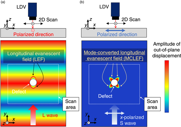
Fig. 1. (Color online) BF and DF imaging methods using the 2D scan of an LDV. The amplitude of out-of-plane displacement (i.e. the z-direction) is shown by the color scale. The scan area is surrounded by a white dotted square. (a) BF imaging method using the LEF excited by L-wave incidence. (b) DF imaging method using the MCLEF excited by the incidence of x-polarized S wave.
Download figure:
Standard image High-resolution imageAs illustrated in Fig. 1(a), the BF imaging method uses an L-wave incidence. When a defect is irradiated by the incident L wave, an LEF can emerge in the vicinity of the defect to satisfy a free-boundary condition at an interface between a solid and air. In the case of a hole, an LEF can be generated on not only the incident side [i.e. the lower surface of the hole, as illustrated in Fig. 1(a)] but also the transmitted side (i.e. the upper surface of the hole) because of the diffraction of the incident wave. Thus, the shadow effect behind a defect (i.e. on the transmitted side) was utilized in past studies. 44,45) However, the propagation of the L wave is also measured by an LDV, since the L-wave propagation has an out-of-plane displacement due to the Poisson effect. Hence, this BF imaging method may not be suitable for achieving a high SNR.
In contrast, the DF imaging method proposed in this study utilizes the incidence of an x-polarized shear (S) wave, as illustrated in Fig. 1(b). In this case, a response does not appear in a defect-free area since an LDV only measures an out-of-plane displacement. In the vicinity of a defect, an evanescent field emerges to satisfy a free-boundary condition. Specifically, a mode conversion from the x-polarized S wave to L wave occurs at the interface. When the incidence angle is above a critical angle, an MCLEF emerges in the vicinity of the interface, as described later in detail. Note that the MCLEF has an out-of-plane displacement, which can be probed by the LDV. In addition, the MCLEF can be generated, even at a defect, that is much smaller than the diffraction limit. Hence, the DF imaging method can achieve high-SNR imaging of micro defects.
To clarify the condition for MCLEF generation, we suppose that an ultrasonic wave propagates from a medium 1 to a medium 2, and there is an interface between the media, 1 and 2 [See Fig. 2]. Although an evanescent field excited in medium 2 under a total reflection condition is well known,
37) the proposed method utilizes an evanescent field excited in medium 1 by the incidence of an x-polarized S wave. To simplify the incidence of the x-polarized S wave onto a defect with air [Figs. 2(a) and 2(c)], we assume that a plane x-polarized S wave propagates to a flat interface between a solid (medium 1) and a vacuum (medium 2) in the orthogonal coordinates defined in Figs. 2(b) and 2(d), respectively.
51) When an incidence angle  of the x-polarized S wave is smaller than a critical angle

which is determined by Snell's law, L and S waves are reflected at the angles of  and
and  , respectively [See Figs. 2(a) and 2(b)]. Here
  and
and  are the speeds of the L and S waves in medium 1, respectively. Note that the L wave is generated because of the mode conversion at the interface. When
  is greater than
  , the mode conversion at the interface generates a longitudinal evanescent field, which can be referred to as the MCLEF, in addition to the reflection of the S wave [See Figs. 2(c) and 2(d)]. The MCLEF is a non-propagating wave field and spatially decays with increasing distance away from the interface. Note that the MCLEF can be generated at any defects for
  , regardless of the size of the defects, which provides us with the potential for super-resolution imaging.
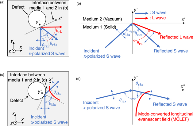
Fig. 2. (Color online) Reflection of an incident x-polarized S wave at the vacuum-solid interface. (a) and (b) Incidence and reflection around a hole and at an interface, respectively, for an incident angle below the critical angle. (c) and (d) Incidence and reflection around a hole and at an interface, respectively, for an incident angle above the critical angle.
Download figure:
Standard image High-resolution image3. Proof of the concept in numerical simulation and experiment
To prove the concept of DF imaging using an MCLEF, we performed numerical simulation based on a 2D FE analysis using a commercial software package (ComWAVE, ITOCHU Techno-Solutions Corporation, Japan). Figure 3(a) shows the FE model. The sample material was an aluminum alloy in which the speeds of L and S waves are 6340 m s−1 and 3140 m s−1, respectively, and which had a simple defect, i.e. a hole with a diameter of 1 mm. An x-polarized S wave (1 MHz, 3 cycle) was emitted upward from the transmitter, positioned at the bottom of the sample. The diameter of the hole was approximately  /3, where
  is the wavelength of the S wave. The Courant number was 0.8 and the mesh size was 0.005 mm. Although the investigation of the out-of-plane (i.e. the z-direction) displacement of the MCLEF that an LDV can measure requires a 3D FE simulation, we regarded the L-wave components calculated in the 2D FE simulation as the out-of-plane displacement to save the computation cost, since only the L-wave components generate out-of-plane displacement because of the Poisson effect. Here, we extracted the longitudinal component from the calculated displacement fields as follows. Based on Helmholtz's theorem,
37) the displacement field
is the wavelength of the S wave. The Courant number was 0.8 and the mesh size was 0.005 mm. Although the investigation of the out-of-plane (i.e. the z-direction) displacement of the MCLEF that an LDV can measure requires a 3D FE simulation, we regarded the L-wave components calculated in the 2D FE simulation as the out-of-plane displacement to save the computation cost, since only the L-wave components generate out-of-plane displacement because of the Poisson effect. Here, we extracted the longitudinal component from the calculated displacement fields as follows. Based on Helmholtz's theorem,
37) the displacement field  can be decomposed into a scalar potential
  and a vector potential Ψ

where  and
and  correspond to the L-wave and S-wave components of the displacement. By taking the divergence of
  , the L-wave component
  can be extracted as

since  . Given the Poisson effect,
  can be treated as an out-of-plane displacement.
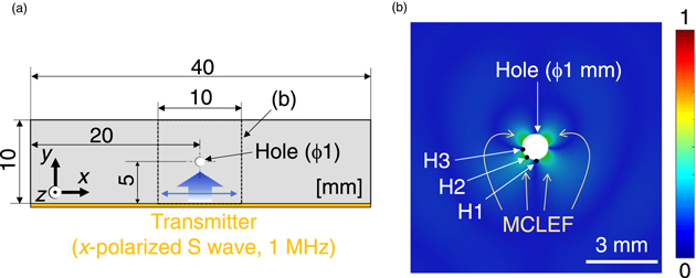
Fig. 3. (Color online) FE analysis of an MCLEF generation behavior around the hole (ϕ1 mm). (a) FE simulation model with the hole. (b) Snapshot of the out-of-plane displacement (i.e. the z-direction) around the hole at t = 2.89 μs. The color scale was normalized to an incident wave amplitude.
Download figure:
Standard image High-resolution imageFigure 3(b) shows the snapshot of the out-of-plane displacement (i.e.  ) in an area of 10 mm × 10 mm at t = 2.89 μs, to simulate the measurement by the 2D scan from the LDV.
50) As a result, strong responses (i.e. the MCLEF) emerged in the vicinity of the hole. Note that the MCLEF did not emerge at H1, corresponding to the incident point for the normal incidence of the x-polarized S wave. As the incidence angle was increased, the MCLEF was strong, for instance, at H2. This position corresponds to the incidence angle above the critical angle (29.8°). On the other hand, the MCLEF was not generated at H3, corresponding to the left edge of the hole. This is because the effective irradiation area of the incident S wave on the hole (i.e. the projective component of the hole surface in the x-direction) was very small around H3. Furthermore, a similar distribution of the MCLEF was observed behind the hole. This can be explained by the diffraction of the incident S wave behind the hole. Note that the incident S wave was not observed. Thus, the simulation results proved the concept of the DF imaging method using an MCLEF.
) in an area of 10 mm × 10 mm at t = 2.89 μs, to simulate the measurement by the 2D scan from the LDV.
50) As a result, strong responses (i.e. the MCLEF) emerged in the vicinity of the hole. Note that the MCLEF did not emerge at H1, corresponding to the incident point for the normal incidence of the x-polarized S wave. As the incidence angle was increased, the MCLEF was strong, for instance, at H2. This position corresponds to the incidence angle above the critical angle (29.8°). On the other hand, the MCLEF was not generated at H3, corresponding to the left edge of the hole. This is because the effective irradiation area of the incident S wave on the hole (i.e. the projective component of the hole surface in the x-direction) was very small around H3. Furthermore, a similar distribution of the MCLEF was observed behind the hole. This can be explained by the diffraction of the incident S wave behind the hole. Note that the incident S wave was not observed. Thus, the simulation results proved the concept of the DF imaging method using an MCLEF.
To validate the FE simulation, we performed a fundamental experiment in the configuration shown in Fig. 4(a). We prepared an aluminum-alloy (A7075) plate with a hole (ϕ1 mm). An S-wave transmitter (1 MHz, ϕ12.7 mm) was placed on the sample edge so that the displacement of the S wave was parallel to the x-direction. We measured the out-of-plane displacement around the hole using an LDV (OFV505, Polytec, Germany), where the 2D mechanical scan of the LDV was performed over an area of 10 mm × 10 mm with a scan pitch of 0.5 mm. As a result, strong responses were observed in the vicinity of the hole, as shown in Fig. 4(b). Note that the 2D pattern of the responses in Fig. 4(b) was similar to that in Fig. 3(b), although the amplitude was different, probably due to the fabrication accuracy of the hole. Thus, we successfully observed the MCLEF generation and validated the results [Fig. 3] calculated by the FE simulation.

Fig. 4. (Color online) Experimental observation of the MCLEF generation around the hole. (a) Experimental condition, (b) Out-of-plane displacement (i.e. the z-direction) around the hole.
Download figure:
Standard image High-resolution image4. FE simulations for demonstrating the super-resolution and high-SNR imaging capability
4.1. Dependence of MCLEF on defect size
To demonstrate the proposed method for micro defects, we varied the hole size (ϕ1 mm, ϕ0.6 mm, ϕ0.3 mm, and ϕ0.15 mm) in the FE model shown in Fig. 3(a). Except for the hole size, we used the same conditions as those used for Fig. 3(a).
Figure 5 shows the snapshots of the out-of-plane displacement in the simulation results for the various hole sizes. Strong responses emerged regardless of the hole size. The MCLEF exhibited a 2D pattern with the same shape, whereas the spatial spreading became smaller with the decrease in the hole size. This is due to the difference in the ultrasonic irradiation area on the hole. Note that the MCLEF can be generated even at a hole with a diameter of 0.15 mm diameter. Thus, we found that the proposed method has a high sensitivity to micro defects that are much smaller than the diffraction limit (i.e. λ/2).
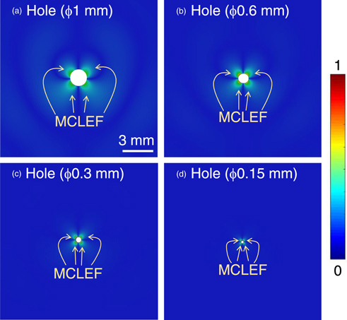
Fig. 5. (Color online) Snapshots of the out-of-plane displacement around holes at t = 2.89 μs calculated by FE simulation. (a) ϕ1 mm (≒λ/3), (b) ϕ0.6 mm (≒λ/5), (c) ϕ0.3 mm (≒λ/10), and (d) ϕ0.15 mm (≒λ/20). The color scale was normalized to an incident wave amplitude.
Download figure:
Standard image High-resolution image4.2. Comparison between BF and DF imaging for various defect geometries
To prove the effectiveness of the proposed method in terms of SNR, we performed the FE simulation using the BF and DF imaging methods, respectively, where the former corresponded to conditions used in past studies. 44,45) Figure 6 shows the FE simulation model with different defect geometries (i.e. a hole, a square, and a crack). We inputted L and x-polarized S waves from the bottom of the sample for the BF and DF imaging methods, respectively. To select the same relationship between the wavelength and the defect sizes, λ was fixed to approximately 3 mm for both methods, where their frequencies were 1 and 2 MHz for the incidence of the L-wave and x-polarized S wave, respectively. We prepared three types of defects: hole, square, and crack. The size of each defect was selected to be comparable to λ/20, which is much smaller than the diffraction limit (i.e. λ/2). The other simulation conditions were the same as those for Figs. 3 and 5.

Fig. 6. (Color online) FE simulation model with various defects for the comparison between the BF and DF imaging methods. (a) FE simulation model. Enlarged models around (b) hole, (c) square, and (d) crack.
Download figure:
Standard image High-resolution imageFigures 7(a)–7(c) show the snapshots of the out-of-plane displacement at 1.43 μs for the L-wave incidence. As a result, the LEF was observed in the vicinity of all the defects. In Fig. 7(a), the LEF emerged in the upper and lower sides of the hole. The LEF in Fig. 7(b) was similar to that in Fig. 7(a), although the spatial distribution was slightly different between them. In Fig. 7(c), the strong LEF emerged around the geometric changes (e.g. upper and lower tips of the crack), whereas an LEF with weaker amplitude emerged in the other parts of the crack. Although the LEFs were observed regardless of the types of defects, the BF imaging method had low SNRs because the incident L wave with the out-of-plane displacement appeared as background.

Fig. 7. (Color online) Snapshots of out-of-plane displacement around defects calculated by FE simulation. BF images for (a) hole, (b) square, and (c) crack at 1.43 μs obtained by L-wave incidence. DF images for (d) hole, (e) square, and (f) crack at 2.89 μs obtained by the incidence of x-polarized S wave. The color scale was normalized to an incident wave amplitude.
Download figure:
Standard image High-resolution image
Figures 7(d)–7(f) show the snapshots of the out-of-plane displacement at 2.89 μs for the incidence of an x-polarized S wave. As a result, the MCLEFs were clearly observed in the vicinity of all of the defects. In Figs. 7(d) and 7(e), the MCLEFs emerged in diagonal directions. The 2D pattern was similar, whereas the amplitude of the MCELF in the vicinity of the square defect was slightly larger than that in the vicinity of the hole. This is probably because the effective area above a critical incidence angle in the square was larger than that in the hole. In Fig. 7(f), strong MCLEFs emerged around the upper and lower parts of the crack. Importantly, the SNRs for the DF imaging method were much higher than those for the BF imaging method, regardless of the type of defect. This is because the incident S wave does not appear as background in Figs. 7(d)–7(f). Thus, we demonstrated the effectiveness of the proposed method in terms of SNR.
5. Discussion
In this study, we demonstrated that the DF imaging method using the MCLEF is useful for achieving a much higher SNR than the BF imaging method using the LEF. Figures 5(d), 7(d)–7(f) also showed the super-resolution imaging capability of the proposed method for defects that were much smaller than the diffraction limit (i.e. λ/2). On the other hand, the spatial spreading of the MCLEF became small with decreased defect size, as shown in Fig. 5. This may cause one to overlook the MCLEF emergence when the scan pitch of the LDV is insufficient. To solve this problem, a large-amplitude incidence would be promising. Given that the MCLEF emergence is a linear phenomenon, a high-intensity region of the MCLEF is spatially increased by increasing the incident wave amplitude. Hence, the proposed method with a large-amplitude incidence will enhance its practical applicability. To realize a large-amplitude incidence, the use of high-voltage excitation, 52) with standing S waves, 53) acoustic metamaterial, 54) and the development of a large-amplitude transmitter 55) will be useful.
In this study, we used surface defects to prove the concept of the proposed method. However, the proposed method could be applied not only to surface defects, but also subsurface defects, as reported for BF imaging. 44,45) Furthermore, the concept of using MCLEF has a potential for markedly enhancing some SLS techniques. 20–22) For such applications, the 3D FE simulation of subsurface defects would be required, to understand the characteristics of a 3D MCLEF before its experimental demonstration, which is one of the exciting future works yet to come.
For the experiment shown in Fig. 4, we emitted the x-polarized S wave at the edge of the sample, which is not practical for on-site applications. Instead, we can use an S-wave transmitter with a wedge. 56) For the reception of the MCLEF, the use of the LDV enables a flexible 2D scan, as demonstrated in this study. However, the 2D scan of the LDV to obtain the results in Fig. 4(b) took approximately 3 h. This is a serious drawback for on-site applications. Note that, to improve the SNR, the acquisition at each receiving point was made after the average of 256 signals via the oscilloscope. A high-speed analog-to-digital converter installed in a PC can shorten the acquisition time to approximately 1/10 of the time taken by using an oscilloscope. Replacing the He-Ne LDV employed in this study with an infrared LDV 57) can markedly enhance the SNR without the need for averaging, which can further shorten the acquisition time. As a different approach, a piezoelectric 2D matrix array transducer 58–63) can be used to probe the MCLEF with an S-wave transmitter, enabling the real-time acquisition of the MCLEF.
6. Conclusions
In this study, we proposed the DF imaging method using MCLEF to visualize surface/subsurface micro defects with a high SNR. After describing the principle of the proposed method, we proved the concept in a specimen with a hole, by FE simulation and fundamental experiment. The further FE simulations demonstrated its super-resolution imaging capability for holes with different sizes and higher SNR than the BF imaging method for various defect geometries.
Acknowledgments
This work was partially supported by JSPS KAKENHI (19K21910, 21H04592) and JST FOREST program (JPMJFR2023).