
Abstract
We analytically studied the Fano resonance in a simple coupled oscillator system. We demonstrate directly from the equation of motion that the resonance profile observed in this system is generally described by the Fano formula with a complex Fano parameter. The analytical expressions are derived for resonance frequency, resonance width, and Fano parameter, moreover conditions under which the Fano parameter becomes a real number are also examined. These expressions, derived for the simple system, are expected to be helpful for considering various other physical systems because the Fano resonance is a general wave phenomenon.
Export citation and abstract BibTeX RIS
In recent years, Fano resonances 1–3) have attracted considerable attention in various artificial quantum structures such as quantum dots, 4) nanowires, and tunnel junctions. 5,6) Fano resonance, which originates from interference between the localized and propagation states, is a general wave phenomenon that does not depend on the nature of the waves. Thus, this resonance has also been studied in various classical systems such as plasmonic nanostructures, 7,8) metal-slit superlattices, 9) photonic crystals, 10,11) and phononic metamaterials. 12–14) In addition, Fano resonances have a wide range of applications, such as sensing and switching. 8,15–17) In particular, the manipulation of the line shape of Fano resonances has useful applications with significant flexibility.
One of the main features of the Fano resonance is its asymmetric line profile, which can be explained by the Fano formula, where the degree of asymmetry is represented by the Fano parameter q. This asymmetric profile is due to the increase in and suppression of the response of the system at very close frequencies. The increase in the response at a particular frequency is commonly seen in well-known Lorentz resonances. 18,19) The simplest model describing the Lorentz resonance is a harmonic oscillator with a periodic external force. 20,21) The suppression of the response is a fundamental characteristic of the Fano resonance. 3,20) The zero amplitude, when a certain resonance condition is satisfied, has been explained using a simple model comprising two weakly coupled harmonic oscillators. This model demonstrates two resonances, with symmetric and asymmetric profiles, near the two eigenfrequencies of the oscillators. However, even for such a simple system, the analytical expression for the Fano parameter was not derived. Derivation of an analytical solution for the simplest system is useful for an essential understanding of Fano resonance in more complex systems. In addition, the analytical solution is expected to be useful for designing various phononic Fano systems for applications in the development of chemical or biological sensors; this is because the Fano resonances are inherently sensitive to changes in geometry or local environment.
In the present study, we theoretically investigate in detail the resonances that occur in two weakly coupled harmonic oscillators. We analytically derive explicit expressions for amplitude profiles near the resonance frequencies to show that the resonance can be described by the Fano formula with a complex Fano parameter. In the original work by Fano 1) and most subsequent studies, the Fano parameter q was implicitly treated as a real number, which is valid only if the system has time-reversal symmetry because the matrix elements defining q can be considered real. In the present system, the equation of motion clearly shows that q is generally a complex number. We examine the conditions under which the Fano parameter becomes a real number and derive simple expressions for the resonance frequencies, resonance widths, and Fano parameters as functions of the given parameters of the system. In addition, we discuss the features of the Fano resonance with a complex Fano parameter by using our explicit expressions.
In this study, we investigate the dynamics of a pair of harmonic oscillators connected by weak springs, described by the following equations of motion:
Here,  is a coupling constant,
  is the friction coefficient,
  is the eigenfrequency of the oscillator
  when there is no attenuation, and
  is the frequency of the periodic external force, which is assumed to act only on oscillator 1. The stationary solutions of Eq. (1) can be obtained in the forms of
  and
and  The amplitudes
  and
and  are calculated as follows:
Joe et al.
20) studied resonance by numerically calculating Eqs. (2) and (3) for  however, the Fano formula describing the resonance profile was not directly derived. Hereafter, we derive the explicit expressions for the profiles of
  and
and  near resonance.
First, we expand the denominator of  around the eigenfrequency
  because the resonance frequency is expected to be close to
  After a straightforward calculation, we obtain

where
and
Equation (4) is valid when the quadratic term of  in the expanded denominator of
  is negligible compared to the linear term. Equation (4) has the form of the Lorentz formula
Here, the resonance frequency  is obtained as

where

is a frequency shift from the eigenfrequency, and the width  of the resonance is represented as

Similarly, we can obtain an expression for  around
  as
as

where
and
The derivation of Eq. (11) is valid only when  For
For  the two oscillators are decoupled, and
  is expressed in the form of Lorentz resonance:
where
and
For  Eq. (11) is in the form of the Fano formula:
Here,  represents

which is the Fano parameter describing the degree of asymmetry,
1) and  and
and  of the Fano resonance are the same as those of the Lorentz resonance for
  which are given in Eqs. (8)–(10). Equation (17) shows that the Fano parameter is generally a complex number, unless
  From Eq. (12), the condition for the Fano parameter to become a real number is
  That is, the condition for
  to be real is that oscillator 2, which acts as a resonator, should vibrate without friction. However, if
  is also zero, then the Fano profile is not seen, as shown later.
The resonance parameters for  can be expressed in simple forms. Based on these results, we can examine the case of
  As the first example, therefore, we consider, in detail, the case where
  which was numerically studied in a previous paper.
20)
which was numerically studied in a previous paper.
20)
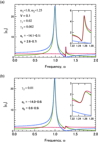
As a numerical example, we show  and
and  in Fig. 1(a), which are calculated from Eqs. (2) and (3) for
  and
and  In Fig. 1(a),
  has an almost symmetric resonance profile and a clear asymmetric profile at frequencies slightly away from
  and
and  respectively. The peak near the eigenfrequency
  of the oscillator, applied with a direct external force, is wider than the asymmetric peak around the eigenfrequency
  of the oscillator, which is coupled with the coupling constant
  In contrast,
  has symmetric profiles near the same resonance frequencies as those for
  Hereafter, we derive the analytical expressions for these resonance profiles to explain their resonance features.
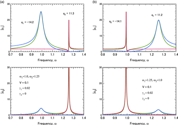
Fig. 1. (Color online) Amplitudes of the first and second oscillators, which are calculated for (a)  and
and  and (b)
  and
and  Solid lines represent values numerically calculated using Eqs. (2) and (3), whereas dotted lines represent values calculated using the analytical expressions, Eqs. (4) and (11) with Eqs. (18) to (23).
Download figure:
Standard image High-resolution imageBy substituting  into Eqs. (5), (12), and (13), and using them in Eqs. (9), (10), and (17), we obtain the explicit expressions for the resonance parameters around
  as
as
and
The frequency shift is proportional to the square of the coupling constant. This is consistent with the analysis of the Fano–Anderson model.
22) The resonance width is also proportional to the square of the coupling constant. The Fano parameter has values proportional to the difference between the squares of the two eigenfrequencies. Within the present approximation, the Fano parameter does not depend on the coupling constant and is inversely proportional to  When friction does not act on first oscillator, the Fano parameter becomes infinite, that is, the resonance peak around
  becomes a Lorentz profile. However, the resonance width
  also becomes zero, and
  diverges at
  In other words, the friction that acts on the first oscillator is necessary for obtaining a resonance profile without divergence.
Similarly, each parameter around  can be obtained in a slightly more complicated form than in Eqs. (18)–(20).
and
The resonance parameters calculated using Eqs. (18)–(23) for the example shown in Fig. 1(a) are as follows: 

 and
and  Numerically calculated resonance frequency shifts using Eqs. (2) and (3) (
 and
and  ) parallel with the analytically obtained results. In addition, we show that the amplitudes calculated using Eqs. (4) and (11) along with Eqs. (18)–(23) in Fig. 1(a), satisfactorily reproduce the numerical results. Here, we note that the above results mathematically indicate that the profile of
  around
  is also a Fano resonance, although the profile looks almost symmetric. This is because the value of Fano parameter is large.
The resonance frequency shifts, such that the two resonance frequencies are separated, that is,  and
and  for
for  can be explained using Eqs. (18) and (21). Furthermore, Eq. (16) shows that the zero point in the Fano resonance is given by
  In contrast, the zero point is
  as shown in Eq. (2) for
  Therefore,
  is negative at resonance around
  and positive around
  that is,
 and
and 
As an example of  Fig. 1(b) shows results for
  As seen in Eqs. (18) and (21),
  and
and  are positive, and
  and
and  are negative for
  That is, the profile around
  has a dip on the right. The resonance parameters are


Next, we consider the case where weak friction acts on oscillator 2 in addition to oscillator 1. Figure 2(a) shows the values of  calculated for
  and
and  The other parameters are the same as those in Fig. 1(a). A large, almost symmetric peak and a small asymmetric peak are observed around
  and
and  respectively. The calculated Fano parameters are
  and
and  and the peak widths are
  and
and  Because the real part of
  has a large value and the imaginary part has a smaller value, the effect of the imaginary part can hardly be discerned. As a result, the profile becomes almost symmetric around
  In contrast, both the real and imaginary parts of
  have a value of approximately 1, leading to an asymmetric peak around
  and the minimum value of the dip has a finite value.
Fig. 2. (Color online) Amplitudes of the first oscillator, which are calculated for (a)  and (b)
  The other parameters are the same as those in Fig. 1(a). Solid lines represent numerically calculated values, whereas dotted lines represent analytically calculated values.
Download figure:
Standard image High-resolution image
Here, we note that the resonance line for the complex value of  is represented by the superposition of the Lorentz and Fano resonances (with a real Fano parameter) of the same resonance frequency and width. This can be seen from the following equation for
The first term on the right-hand side of Eq. (24) becomes zero at  giving a dip in the resonance profile, but the minimum value of the dip has a finite value owing to the Lorentz function of the second term. That is, this non-zero minimum value is determined by the imaginary part of the Fano parameter, which originates from
  Figure 2(a) demonstrates that when
  is sufficiently small, a sharp dip with a finite minimum value can be observed. Conversely, if the friction acting on the resonator is considerably strong, no clear Fano profile can be observed. For comparison, the results for
  are shown in Fig. 2(b). The calculated Fano parameters are
  and
and  When the value of
  increases, that of
  attains higher value than
  and the antisymmetric profile becomes less noticeable. Compared to Fig. 2(a), the difference between the analytical and numerical results is larger around
  This is because the tail of the peak around
  overlaps with the considerably small peak around
  Here, we note that
  should be satisfied for the two peaks to be seen clearly and also described accurately.
To summarize, we theoretically investigated the resonance line shapes in mechanical systems of two coupled oscillators under an external harmonic force. The amplitude of the oscillator that acts as a resonator exhibits a symmetric line shape, represented by the Lorentz function; in contrast, the amplitude of the oscillator, to which an external force is applied, exhibits an asymmetric line shape, represented by the Fano formula. The Fano parameter q that describes the asymmetry is generally a complex number.
We derived the analytical formulae for the resonance frequency, resonance width, and Fano parameter q. Subsequently, we also examined the conditions under which q was a real number and indicated that the resonance amplitude of the oscillator with a periodic external force can be described by a Fano formula with a real q when no friction acts on the resonator. These expressions can be presented in a simple form when q is a real number. On the other hand, when friction acts on the resonator, the expression for a complex q is not straightforward, even though the system is simple. The complex q signifies that the resonance line is represented by the sum of the Lorentz and Fano resonances (with a real q) of the same resonance frequency and width, so that the minimum value of the resonance line is not zero. If the friction acting on the resonator is low, a sharp dip with a non-zero minimum is observed. At the limit of zero friction, it becomes a Fano resonance with real q. In other words, the non-zero minimum value of the dip represents the magnitude of the friction acting on the resonator. Furthermore, when the friction, acting on the oscillator when applied with external force, is negligible, the resonance amplitude is expressed in the form of Lorentz resonance.
The examined system is simple but significant for the physical representation of resonance. Our explicit formulae are not only helpful for understanding the Fano resonance in this system, but are also expected to be useful for considering other physical systems. In particular, these are expected to be helpful for controlling the line shape of the Fano resonances.
Acknowledgments
This work was partially supported by JSPS KAKENHI (Grant No. 20K0534100).