

Abstract
Spatial distribution of sonochemiluminescence (SCL) from an argon-saturated luminol solution was measured in a focused sound field at 1 MHz in a standing-wave configuration. The SCL distribution was confined to pre-focal region at acoustic powers lower than 0.9 W, and was not located at the focus but at a few mm pre-focal side at a threshold for SCL inception. The threshold pressure amplitude for SCL inception was 3.6 atm at the focus, which value was obtained with a background-oriented schlieren method. The method is based on the broadening of multiple slits due to an optical deflection caused by ultrasound, and the broadening width measured provides an acoustic pressure amplitude. A qualitative image of the focused sound field was also obtained.
Export citation and abstract BibTeX RIS
1. Introduction
Irradiation of intense ultrasound into liquid generates bubbles that undergo an oscillation of expansion and contraction synchronizing with the acoustic cycle. Acoustic cavitation bubbles can grow from undissolved gas and/or vapor, stabilized on solid surfaces, owing to the reduction of pressure in the negative part of the acoustic cycle. An explosive expansion and contraction of the bubble may provide the conditions of high temperature of several thousand degrees Kelvin and high pressure of several hundred atmospheres via adiabatic process inside the bubble. These extreme conditions cause shock-wave propagation around the bubble, liquid jet, free-radical production and light emission (sonoluminescence). 1,2) Acoustic cavitation by focused ultrasound has been interested in an association with its medical applications: tissue imaging and therapy. 3,4) For tissue imaging, the cavitation is unwanted because the cavitation effect such as OH-radicals production may cause damages to the tissue for diagnosing. On the other hand, the cavitation event is favorable in a therapy application by high-intensity focused ultrasound (HIFU). The heating induced by cavitating bubbles enhances tissue coagulation, which helps to damage a lesion. 5,6)
Numerous studies have been performed to establish the threshold of sound pressure for cavitaion inception. 7–12) Apfel and Holland 13) obtained the theoretical threshold pressure required for cavitation to occur as a function of preexisting nuclei radius. According to their result, a minimum value of the threshold pressure amplitude at 1 MHz is approximately 3 atm for nuclei radius of 0.5–1.0 μm. An exploration of the threshold pressure in a focused field was made by Apfel's group using a passive cavitation detector or active cavitation detector in various conditions of pulse duration and repetition frequency. These works were used to define a mechanical index which was adapted as a measure for evaluating the potential for cavitation in diagnostic ultrasound equipment. 14)
Sonochemiluminescence has been utilized to visualize cavitation field 15,16) and also to detect cavitation inception. 17,18) The high-temperature and high-pressure conditions inside the bubble produce OH and H radicals formed by the pyrolysis of water molecules. OH radicals diffuse out of the bubbles and react with foreign molecules. An excited state of luminol produced by reactions with OH radicals emitting bluish light peaked at 430 nm 19) which is called sonochemiluminscence (SCL). The intensity of SCL is larger than that of sonoluminescence by two orders of magnitude, 20) which is advantageous for detecting the cavitation event to occur. Hallez et al. 21) used SCL to measure the ultrasonic power emitted by HIFU transducer designed for sonochemistry application and they confirmed that the spatial distribution of ultrasonic intensity is qualitatively depicted by SCL.
A spatial distribution of SCL in a focused field was complicated depending on the sound power and sound field condition, i.e. traveling wave or standing wave. 22,23) In a configuration of a traveling wave, cavitating bubbles are pushed away by acoustic radiation force or streaming especially near the focal zone where the acoustic pressure is large. Considering that bubbles are not pushed away in vivo situations, the configuration of standing wave should be tested. It is necessary to know not only the threshold pressure for cavitation inception but also the location of cavitation inception in a focused field, but no such study has been reported. We determined the threshold acoustic pressure and location for SCL in 1 MHz focused sound field in the standing-wave configuration. In the present study, the distribution of focused sound field was obtained by using background-oriented shlieren imaging. 24,25) This method is based on optical deflection of a background pattern caused by ultrasound. Sound pressure amplitude at the focus was estimated from the broadening of the background pattern. A line grid was used as the background pattern in the present experiment.
2. Methods
An aqueous solution of 1 mM luminol (3-aminophthalhydrazide) with adding 48 mM sodium carbonate for adjusting pH to be 12 was degassed and saturated with argon. The solution was contained in a stainless-steel vessel (width: 140 mm, depth: 84 mm, height: 84 mm) equipped with glass windows. A ceramic transducer (Fuji ceramics Co.) with a diameter of 30 mm and a curvature radius of 40 mm was mounted at the side of the vessel. A 0.98 MHz continuous signal from a function generator (Tektronix, AFG1000) was amplified by 53 dB using a power amplifier (E & I, 2100L), impedance-matched with a transformer and fed to the transducer. The photographs of SCL were captured using a digital camera (Nikon D500) with a F/1.2D, 50 mm lens. The exposure time was 30 s and the maximum sensitivity was ISO 64 000. The experimental setup is shown in Fig. 1.
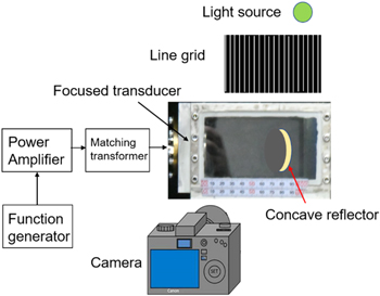
Fig. 1. (Color online) Experimental setup for the measurements of SCL and acoustic pressure.
Download figure:
Standard image High-resolution imageAn inception of acoustic cavitation depends on the existence of bubble nuclei. The initial measurement of SCL was performed at a function-generator output of 200 mV, which is much higher than a threshold output for SCL to occur. The output voltage was then decreased and the SCL photographs were captured. This process repeated without turning off the output until no SCL was observed. This procedure ensures that sufficient numbers of bubble nuclei survive in each SCL measurement. After the series of measurements with decreasing voltage were made, the output broke for two minutes over which time the remaining microbubbles as nuclei disappeared. The SCL measurements again repeated with increasing the output voltage. The electrical power was obtained from the measurements of current and voltage at the transducer. At the output voltage of 100 mV the electric power was measured to be 1.8 W, corresponding to approximately 0.9 W of acoustic power because the efficiency of electrical-acoustic power transduction was about 50%. Measurements were made at a temperature of 24 °C–26 °C. The temperature rise after measurements was within 2 degrees. For satisfying a traveling-wave configuration, an absorbing rubber plate (>40 dB, Eastek EUA101A) was positioned at the end of the vessel to minimize ultrasound reflection. For satisfying a standing-wave configuration, a stainless-steel concave reflector with the same size and the same curvature radius as the transducer was opposed confocally with respect to the transducer. The position of the reflector was adjusted to obtain a maximum pressure by using a XYZ-axis stage.
Using a calibrated hydrophone, the measurement of acoustic pressure can be performed in the traveling wave configuration. However, the hydrophone measurement cannot be performed in the standing-wave configuration because a hydrophone severely disturbs the standing-wave field. We employed, therefore, a noninvasive optical technique: a background-oriented schlieren method, which is based on the effect of optical deflection by ultrasound. 26–28) A pattern of black lines (a line grid) with a width of 1.0 mm and an interval of 1.5 mm was printed on a transparent plastic sheet with an ink-jet printer. This acts as multiple slits with a width of 0.5 mm. As shown in Fig. 1, the line glid was located parallel to the direction of ultrasound propagation with a distance of 200 mm. The line grid was backlighted by a green LED source, providing the lines of light. While interacting with ultrasound, the light was deflected because the spatial variation of refractive index in water was produced by ultrasound pressure. The deflection angle θ of light is given by Refs. 26,27.

where  is the wavelength of sound, L is the length of interaction between light and sound, and P0 is the sound pressure amplitude.
  is the change in refractive index by unit pressure in water, which value is 1.54 × 10⁻¹⁰ Pa−1 at 25 °C. Because an acoustic pressure varies along a light path, the integration along the light path should be introduced. The line glid image captured by a camera, positioned at the other side of the ultrasound vessel, was then blurred because the image was the time average of the deflection effect. Hargrove et al.
26) obtained the time-average intensity of the deflection from a slit with a width of a:
is the change in refractive index by unit pressure in water, which value is 1.54 × 10⁻¹⁰ Pa−1 at 25 °C. Because an acoustic pressure varies along a light path, the integration along the light path should be introduced. The line glid image captured by a camera, positioned at the other side of the ultrasound vessel, was then blurred because the image was the time average of the deflection effect. Hargrove et al.
26) obtained the time-average intensity of the deflection from a slit with a width of a:

Here,  is a nth-order Bessel function, and W
n
is a spread function given by
is a nth-order Bessel function, and W
n
is a spread function given by

where  is the ratio of slit width to sound wavelength. H is a continuous variable describing the distance across the image. Raman–Nath parameter v is defined by

where  is the wavelength of light.
In the present experiment, slits with various width were tested and the width of 0.5 mm was chosen because it showed the light intensity changes enough to distinguish the pressure change both experimentally and theoretically. 26) The interval of the slit was determined to coincide with the sound wavelength of 1.5 mm at 1 MHz. The blurred image provides the time average of the deflection effect, and the width of the blurred image is given by the product of the deflection angle and the distance D between the line glid and the central axis of ultrasound which was set to be D = 200 mm. The deflection angle obtained from the blurred image gives the sound pressure amplitude at the focus using Eq. (1).
The interaction length L was estimated from the calculation of ultrasound field at the focus: the pressure profile of the main lobe along the light path was approximated by the square profile with the height of the maximum peak pressure and the width of L. 29) The value of L that equalize the cross-section of both profiles was obtained to be 2.95 mm. The contributions from neighboring side lobes were neglected because each of them has a out-of-phase nature which cancels the contribution to deflection. In the traveling-wave configuration, the value of acoustic pressure amplitude obtained at the focus was compared with that measured by a calibrated needle hydrophone (Onda, 80-0.5-40) with a sensing diameter of 0.5 mm.
3. Results and discussion
3.1. Threshold pressure for sonochemiluminescence
Typical photographs of SCL are shown in Fig. 2 for output voltages of 200 mV, 150 mV, 100 mV and 56 mV. Red curves in the top figure denote the positions of the transducer (left-hand side) and the concave reflector (right-hand side). Inception of acoustic cavitation has been known to exhibit a hysteresis effect with respect to the applied voltage 30,31) because of the difference in cavitation nuclei number. When the output voltage of 200 mV, which was much larger than a threshold value, was applied, the SCL distribution covered nearly the whole acoustic field. At 150 mV, the area of the SCL distribution became to be narrow. At 100 mV, the SCL distribution was confined to the pre-focal region. The SCL distribution approached the focal zone as the output voltage decreased. At 56 mV, the SCL distribution was located at a few mm pre-focal side from the focus. No SCL was observed below the output of 56 mV, which was regarded as the threshold voltage. In all the photographs captured, stripe patterns with an interval of 0.75 mm were recognized, indicating that cavitating bubbles were trapped at antinodes of the standing wave. These results are in contrast to those in the traveling-wave configuration, where the SCL intensity was much smaller and the SCL distribution was almost located in the post-focal region. Another difference is the existence of acoustic streaming in the traveling-wave configuration. The excessive streaming may push away cavitating bubbles to post-focal region, causing a smaller SCL intensity. Yin et al. 23) observed SCL in the focused sound field at 1.2 MHz in a standing-wave configuration and reported that the SCL distribution extended both pre- and post-focal regions. Their measurements were made at acoustic powers over 10 W, and hence their result agrees with the present result at 200 mV at which the acoustic power is approximately 3.6 W. Hallez et al. 21) also reported SCL in the focused sound field at 0.75 MHz in a free-surface condition at acoustic powers over 8 W. Their experimental situation was a partly standing-wave configuration, and the SCL distribution was similar to the present result. All these studies reported the absence of SCL in the focus. In this respect, Hallez et al. discussed that a high bubble velocity in the focal zone leads to bubble deformation causing insufficient production of OH radicals. The present experiment was performed at powers much lower than those in previous studies and showed the possibility of the OH radical production near the focal zone at acoustic powers lower than 1 W.

Fig. 2. (Color online) Photographs of SCL due to focused ultrasound at 1 MHz in a standing-wave configuration with output voltages of 200 mV, 150 mV, 100 mV, and 56 mV. The threshold voltage was 56 mV.
Download figure:
Standard image High-resolution imageFigure 3 shows the dependence of the SCL intensity on the output voltage. The SCL intensity was obtained from an integration of the brightness of each image pixel using ImageJ software. The threshold voltage of SCL was 56 mV in the series of decreasing voltage (open circles), and 152 mV in the series of increasing voltage (closed squares). This difference in the threshold voltage is explained by the number of cavitation nuclei. In the series of decreasing voltage, the voltage higher than a threshold can create many cavitation bubbles which survive and act as nuclei in the next run. In the series of increasing voltage, however, little nuclei exist before sonication, and the threshold depends on how the liquid was prepared and hence it showed little reproducibility. 8) In the present experiment, no special caution was paid in the preparation of sample liquid except the use of deionized water with 0.2 μm filtering. The reproducibility of the threshold voltage in the series of decreasing voltage was within 10%, and that in the series of increasing voltage was over 50%.
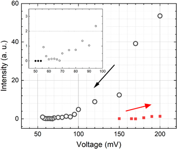
Fig. 3 (Color online) SCL intensity as a function of the output voltage. The open circles denote the SCL intensity as decreasing voltage, and the closed squares denote the SCL intensity as increasing voltage. The open circles are plotted in an expanded scale in the inset. The closed circles indicate no SCL.
Download figure:
Standard image High-resolution image3.2. Acoustic pressure measurement
A calibrated hydrophone is frequently used for measuring acoustic pressure amplitude. A sensor tip of the needle-type hydrophone should be faced to the wavefront of ultrasound to be measured. In the present configuration of the standing wave, the hydrophone measurement was impossible because of the existence of the reflector. Further, the insertion of a hydrophone extremely disturbs a standing-wave field. We employed, therefore, a background-oriented schlieren method to obtain a focused sound-pressure field and to measure acoustic pressure amplitude. Figure 4(a) shows an expanded view of the line grid image blurred by focused ultrasound at the output voltage of 200 mV. The slit width used was 0.3 mm. Figure 4(b) shows the color-coded image of the focused sound field obtained by this method. Using the ImageJ software, a different process was made between the image shown in Fig. 4(a) and that in the absence of ultrasound. Then the pixel brightness was converted to 16 color codes. Because the image of Fig. 4(b) is contributed from the averaging along the optical path, the image demonstrates a qualitative view of the focused sound field. However, the focal zone can be clearly identified.
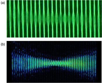
Fig. 4. (Color online) (a) Line grid image deflected by focused sound with an output voltage of 200 mV. (b) Image of focused sound field obtained after the subtraction between sonicated and non-sonicated images and the color-coded process.
Download figure:
Standard image High-resolution imageFigure 5 shows the time-average intensity of the deflection image calculated using Eqs. (2)–(4) for the Raman–Nath parameters v = 0–5 and G = 0.33, i.e. the slit width is 0.5 mm. The case for v = 0 corresponds to a slit image in the absence of ultrasound, and the case for v = 5 to that at an acoustic pressure amplitude of approximately 10 atm in the present experimental condition. The figure indicates that considerable variations in the deflection intensity can be realized except the range of v < 1. The amount of optical deflection resulted from the integration of refractive-index change through the range of interaction with ultrasound. Hence, the contributions from out-of-phase part of ultrasound cancel each other. The phase of ultrasound in the focal zone is nearly constant 28) so that the magnitude of the deflection in the focal zone shows appropriately the real pressure amplitude. A quantitative evaluation of the sound field was difficult except for the focal zone, where the ultrasound phase is not constant along the light path because of the spherical-wave nature of focused ultrasound.
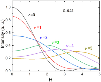
Fig. 5. (Color online) Time-average intensity of the deflection image calculated using Eqs. (2)–(4) for the Raman–Nath parameters v = 0–5 and G = 0.33.
Download figure:
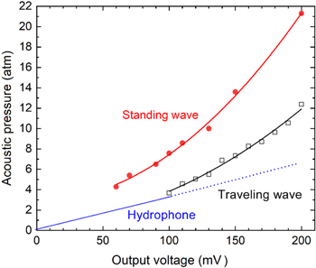
Standard image High-resolution imageWe obtained an acoustic pressure amplitude from a blurred slit image, such as shown in Fig. 4(a), at several output voltages in the standing-wave and traveling-wave configurations, as shown in Fig. 6. The values for the standing wave were 1.8 times larger than those for the traveling wave, and both values were fitted by quadratic curves. The accuracy of these results was determined by the comparison with the measurement by a calibrated hydrophone. The hydrophone measurement was made at the output voltage from 50 to 100 mV in a burst-wave mode and the traveling-wave configuration. The pressure amplitudes measured were 1.74 atm at 50 mV and 3.20 atm at 100 mV. The present result of pressure amplitude was 3.8 atm at 100 mV in the traveling-wave configuration, which is 20% larger than that by the hydrophone. This discrepancy is attributed to the unclear boundaries of deflection intensity caused by the slit effect, as shown in Fig. 5. The quadratic property of the output-voltage dependence may be attributed to a finite amplitude effect of focused ultrasound. 32,33) The content of the second-harmonic component was measured to be 3% at 100 mV in the traveling-wave configuration. A quantitative analysis of the broadened image should be required to compare with the calculated intensity shown in Fig. 5. Then we conclude that the present method can be applied to the measurement of pressure amplitude using the calibration curve as shown in Fig. 6.
Fig. 6. (Color online) Acoustic pressure obtained by a background-oriented schlieren method in the standing-wave (closed circles), and traveling-wave (open squares) configurations. The results by hydrophone measurements are indicated by the blue line.
Download figure:
Standard image High-resolution image
3.3. Threshold acoustic pressure
The threshold of acoustic pressure for SCL can be estimated from the above measurements. From Fig. 6, the acoustic pressure amplitude corresponding to the output of 56 mV is 4.3 atm in the standing-wave configuration, and this value should be reduced to 4.3/1.2 = 3.6 [atm] because the experimental value is close to 4.3 atm in the traveling-wave configuration is larger than the calibrated value by 20%. Apfel's group reported the threshold pressure using a passive cavitation detector or active cavitation detector in various conditions of pulse duration and repetition frequency. Atchley et al. 11) demonstrated the threshold pressure of approximately 5 atm for 0.98 MHz focused ultrasound with 1 ms duration and 10 Hz duty cycle. Roy et al. 12) showed that an active cavitation detector yields threshold values that were less than or equal to those measured by a passive detector. Carmichael et al. 34) performed electron spin resonance measurements of free radical production due to plane continuous-wave (CW) ultrasound at 1 MHz. The threshold ultrasound intensity that they obtained was 0.7–1.4 W cm−2 which is corresponding to 1.4–2.0 atm. This threshold value is lower than that obtained by other studies. A different condition with the present experiment was the use of a traveling plane wave. Fowlkes and Crum 17) determined the threshold pressure for SCL in an argon-saturated luminol solution. They used microsecond-length pulses of 1 MHz focused ultrasound in a traveling-wave configuration. A light detection was made with a photon-counting system. Extrapolation of their result to CW condition gives a threshold pressure of 4.4 atm, which roughly agrees with the present result. Hallez et al. 21) reported that a threshold pressure in air-saturated solution is 20% larger than that in argon-saturated solution. The present result is in reasonable agreement with the previous results. The use of a more sensitive detector employing an image intensifier may lead to a lower threshold value.
4. Conclusions
The present study showed that SCL spatial distribution in a focused field changed with acoustic power. The location of SCL approached to focal zone as acoustic power decreased, but did not correspond to the focus at a threshold pressure. This indicates that the inception of SCL depends on not only acoustic pressure but also other effects such as streaming velocity. Acoustic pressure amplitude in the focal zone was determined with a background-oriented schlieren method, which was calibrated by a needle hydrophone. Although this method gives only a qualitative image of the focused sound field, the experimental setup is simple and easy to be constructed. It will be profitable to monitor the sound field in a small glass cell immersed in a large container, which may be used for ultrasound irradiation to a small quantity of the sample.
Acknowledgments
This work was supported by the Project of International Collaborative Research Promotion, Meiji University. The authors thank Hyang-Bok Lee for her useful discussion.