
Abstract
We developed the coupled calculation of plasma and gas flows in simulations for dual-frequency excited Ar/SF6 plasma. By focusing on the effect of secondary electron emission (SEE), we varied SEE coefficient γ and determined γ = 0.04 from the comparison of calculation results with the experimental results. The dependence of electron density on spatial distribution and SF6 gas partial pressure was compared between calculation and experimental results. As a result, at SF6 = 5.0 sccm, the calculated electron densities at the center and edge were almost the same as the experimental results. Furthermore, at SF6 = 2.5 sccm, the error from the experiment including the spatial distribution was in the range of −11.03 to 4.11%, and the results of coupled calculation of plasma and gas flows in simulations can reproduce the experimental results under at a SF6 partial pressure in the range from 2.5 to 5.0 sccm.
Export citation and abstract BibTeX RIS
1. Introduction
With the miniaturization of semiconductors, the control of the etching shape with high accuracy is required. 1,2) In addition, from the viewpoint of improving productivity, an etching process that improves yield and shortens process time is expected. 3) To meet these requirements, research studies to increase plasma density and the controllability of the etching plasma source are being conducted actively. 4,5)
As a plasma source for etching, a capacitively coupled plasma apparatus in which an RF voltage is applied to the lower electrode placed on a wafer is widely used. To improve the plasma density and controllability, a dual-frequency plasma source in which RF power supplies of different frequencies are connected to the upper and lower electrodes has been proposed. 6–9) In this method, a high-frequency RF power supply is connected to the upper electrode to generate high-density plasma. On the other hand, a low-frequency RF power supply is connected to the lower electrode to control Vdc. By adjusting the RF frequency and voltage of the upper and lower electrodes, we can generate the plasma required for etching.
Plasma simulation is effective for improving the efficiency of the development of a plasma etching apparatus and the optimization of plasma states. By plasma simulation, we can visualize the distributions of electron density, ion density, and active species density. 10–14) Several simulations have been reported so far for dual-frequency plasmas. Lee et al. showed the difference in plasma parameters between single-frequency and dual-frequency plasmas by simulation. 15) Rebiaï et al. investigated the effects of high-frequency and low-frequency power supplies on plasma parameters by simulation using a two-dimensional (2D) model. 16) Moreover, in dual-frequency capacitively coupled plasmas, interest has been increasing on the effect of secondary electron emission (SEE) due to collisions between electrodes and positive ions, and many studies have been reported. 17–19)
However, in the simulation of dual-frequency plasma, there are only a few studies in which gas flow and SEE are taken into consideration and compared with the measured plasma density. In our previous study, we performed a coupled calculation of simulation of plasma and gas flow in a dual-frequency excited Ar gas plasma and compared the calculation results with the experimental results. 20) As a result, the effects of Ar* diffusion on the exhaust port and SEE were confirmed. 20)
In this study, we applied the coupled calculation of plasma and gas flow simulation to an Ar/SF6 mixed gas, which is used for etching and has a more complicated gas reaction. In particular, by focusing on the SEE effect, we compared the experimental results with the coupled calculation results using the SEE coefficient as a parameter. As a result, it was shown that the dependence of electron density on spatial distribution and SF6 gas partial pressure can be reproduced by setting the SEE coefficient to 0.04.
2. Experimental methods
A dual-frequency capacitively coupled plasma apparatus was used in the experiment. Figure 1 shows a cross section of the apparatus. The diameter of the lower electrode is 4 inches, and the process gas is supplied from the upper electrode. The gas flow rates were Ar/SF6 = 50/2.5 and Ar/SF6 = 50/5.0 sccm, and the total pressure was set to be 4 Pa for both gas mixtures. Both the upper electrode and the lower electrode have a structure in which the metal material is covered with Si. The upper electrode was insulated from the ground (GND) of the chamber using Teflon and the lower electrode was insulated from the GND using alumina. The frequencies of the upper and lower electrodes were 60 and 2 MHz and the input powers were 400 and 500 W. When input powers of 400 and 500 W were applied to the upper and lower electrodes, the RF voltages were 810 and 905 Vpp, respectively,

Fig. 1. Cross section of dual-frequency capacitively coupled plasma apparatus. Reproduced from Ref. 20. © 2021 The Japan Society of Applied Physics.
Download figure:
Standard image High-resolution imageThe electron density was measured using an absorption probe. 21,22) The absorption probe had an antenna diameter of 0.5 mm and a length of 10 mm, and the outer diameter of the glass covering the antenna was 4 mm. As shown in Fig. 1, the tip of the probe antenna was located at the center of the chamber (CNT) and 35 mm away from the center (EDG). The center of the absorption probe was set at 23 mm over the lower electrode. The electron densities at CNT and EDG were measured at a constant gas pressure of 4 Pa and SF6 flow rates of was 2.5 and 5.0 sccm. The electron densities at CNT and EDG at the SF6 flow rate of 2.5 sccm were 14.6 × 10¹⁶ and 13.6 × 10¹⁶ m−3, respectively. The electron densities at CNT and EDG at the SF6 flow rate of 5.0 sccm were 10.2 × 10¹⁶ and 8.5 × 10¹⁶ m−3, respectively.
3. Simulation model
3.1. 2D model configuration and boundary conditions
Figure 2 shows the simulation model. One-half of the cross section of the chamber was used as a simulation model. The central axis of the chamber corresponded to the center of the cylindrical coordinates, and the vertical and lateral directions were defined as the z- and r-axes, respectively. In this coordinate system, the position of the absorption probe at the center was (r, z) = (0, 80) and that at the edge was (r, z) = (35, 80).

Fig. 2. (Color online) 2D plasma simulation model. 20)
Download figure:
Standard image High-resolution imageThe boundary conditions for the simulation were set to be the same as those for experiment. The gas mixture Ar/SF6 was set to be evenly supplied from the upper electrode and exhausted from the space between alumina and the chamber (lower right of Fig. 2). The gas flow rates were Ar/SF6 = 50/2.5 and Ar/SF6 = 50/5.0 sccm, and the total pressure was set to be 4 Pa for both gas mixtures. The relative permittivity of the insulating material Teflon of the upper electrode was 2.5, and that of alumina was 8.5. A frequency of 60 MHz and Vpp = 810 V were applied to the upper electrode, and a frequency of 2 MHz and Vpp = 905 V were applied to the lower electrode. The other metal surfaces were grounded.
3.2. Plasma simulation
Plasma hybrid module (PHM) of Pegasus Software Inc. was used as the fluid model for the plasma simulation. In PHM, the continuity equation of electrons is expressed as

where  is the electron density,
  is the electron flux, and
  is the electron generation rate. Similarly, the ion density
  is given as

where  is the ion flux and
  is the ion generation rate.
The gas reaction model in the plasma simulation was constructed referring to Refs. 23–26. Table I shows the species calculated in the simulation. Twenty-four types of ion and radical generated from SF6, F2, and Ar were calculated in the simulation. Table II summarizes the reactions of electrons with molecules, atoms, neutral radicals, and ions. Thirty-five types of reaction were incorporated into the plasma simulation referring to the reaction constants in Refs. 23–33. Table III shows the reactions between ions, molecules, and atoms. Sixty-four types of reaction were incorporated into the plasma simulation, mainly referring to the reaction rates in Refs. 27 and 34.
Table I. Species considered in Ar/SF6 gas reaction model.
| Molecules atoms | Ions | Radicals |
|---|---|---|
| SF6 | SF5 +, SF4 +, SF3 +, SF2 +, SF+, S+ | SF5, SF4, SF3, SF2, SF, F |
| SF6 −, SF5 −, SF4 −, SF3 −, SF2 − | ||
| F2 | F2 +, F+ | F |
| F2 −, F− | ||
| Ar | Ar+ | Ar* |
Table II. Electron impact collisions included in Ar/SF6 gas reaction model.
| Reaction number | Reaction | References |
|---|---|---|
| G1 | e + SF6 → SF6 + e | 24 |
| G2 | e + SF6 → SF5 + + 2e + F | 25 |
| G3 | e + SF6 → SF4 + + 2e + 2F | 25 |
| G4 | e + SF6 → SF3 + + 2e + 3F | 25 |
| G5 | e + SF6 → SF2 + + 2e + 2F +F2 | 25 |
| G6 | e + SF6 → SF+ + 2e + 3F + F2 | 25 |
| G7 | e + SF6 → S+ + 2e + 4F + F2 | 25 |
| G8 | e + SF6 → F+ + 2e + 4F + SF4 | 25 |
| G9 | e + SF6 → SF6 − | 24 |
| G10 | e + SF6 → SF5 − + F | 24 |
| G11 | e + SF6 → SF4 − + 2F | 24 |
| G12 | e + SF6 → SF3 − + 3F | 24 |
| G13 | e + SF6 → SF2 − + 4F | 24 |
| G14 | e + SF6 → F− + SF4 + F | 24 |
| G15 | e + SF6 → F2 − + SF4 | 24 |
| G16 | e + SF6 → SF3 + e + 3F | 27 |
| G17 | e + SF6 → SF2 + e + 4F | 27 |
| G18 | e + SF6 → SF5 + F− | 24 |
| G19 | e + SF6 → F2 − + SF4 | 24 |
| G20 | e + SF5 → SF5 + + 2e | 23 |
| G21 | e + SF5 → SF4 + + 2e + F | 23 |
| G22 | e + SF4 → SF4 + + 2e | 23 |
| G23 | e + SF3 → SF3 + + 2e | 23 |
| G24 | e + SF2 → SF2 + + 2e | 23 |
| G25 | e + SF → SF+ + 2e | 23 |
| G26 | e + F2 → F2 + e | 30 |
| G27 | e + F2 → F−+ F | 30 |
| G28 | e + F2 → F + F + e | 30 |
| G29 | e + F2 + → F + F | 30 |
| G30 | e + F →F+ + 2e | 31 |
| G31 | e + S → S+ + 2e | 29 |
| G32 | e + Ar → Ar + e | 32 |
| G33 | e + Ar → Ar+ + 2e | 33 |
| G34 | e + Ar → Ar* + e | 33 |
| G35 | e + Ar* → Ar+ + 2e | 33 |
Table III. Reactions between ions, molecules, and atoms included in Ar/SF6 gas reaction model.
| Reaction number | Reaction | References |
|---|---|---|
| G36 | F− + F → F2 + e | 27, 34 |
| G37 | F− + F → 2F + e | 27, 34 |
| G38 | F− + F2 → F + F2 + e | 27, 34 |
| G39 | F2 − + F → F2 + F +e | 27, 34 |
| G40 | F2 − + F2 → 2F2 + e | 27, 34 |
| G41 | F− + F2 + → F + F2 | 27, 34 |
| G42 | F− + F+ → F + F | 27, 34 |
| G43 | Ar+ + F− → Ar + F | 27, 34 |
| G44 | F+ + F2 → F2 + + F | 27, 34 |
| G45 | F2 + + F2 → F2 + + F2 | 27, 34 |
| G46 | F+ + F2 − → F + F2 | 27, 34 |
| G47 | F2 + + F2 − → 2F2 | 27, 34 |
| G48 | SF+ + F− → SF + F | 27, 34 |
| G49 | SF2 + + F− → SF2 + F | 27, 34 |
| G50 | SF3 + + F− → SF3 + F | 27, 34 |
| G51 | SF4 + + F− → SF4 + F | 27, 34 |
| G52 | SF5 + + F− → SF5 + F | 27, 34 |
| G53 | SF+ + F2 − → SF + F2 | 27, 34 |
| G54 | SF2 + + F2 − → SF2 + F2 | 27, 34 |
| G55 | SF3 + + F2 − → SF3 + F2 | 27, 34 |
| G56 | SF4 + + F2 − → SF4 + F2 | 27, 34 |
| G57 | SF5 + + F2 − → SF5 + F2 | 27, 34 |
| G58 | SF6 − + F+ → SF6 + F | 27, 34 |
| G59 | SF6 − + SF+ → SF6 + SF | 27, 34 |
| G60 | SF6 − + SF2 + → SF6 + SF2 | 27, 34 |
| G61 | SF6 − + SF3 + → SF6 + SF3 | 27, 34 |
| G62 | SF6 − + SF4 + → SF6 + SF4 | 27, 34 |
| G63 | SF6 − + SF5 + → SF6 + SF5 | 27, 34 |
| G64 | SF6 − + F2 + → SF6 + F2 | 27, 34 |
| G65 | SF5 − + F+ → SF5 + F | 27, 34 |
| G66 | SF5 − + SF+ → SF5 + SF | 27, 34 |
| G67 | SF5 − + SF2 + → SF5 + SF2 | 27, 34 |
| G68 | SF5 − + SF3 + → SF5 + SF3 | 27, 34 |
| G69 | SF5 − + SF4 + → SF5 + SF4 | 27, 34 |
| G70 | SF5 − + SF5 + → SF5 + SF5→ | 27, 34 |
| G71 | SF5 − + F2 + → SF5 + F2 | 27, 34 |
| G72 | SF5 + + SF6 − → SF3 + + SF6 + F2 | 27, 34 |
| G73 | SF + F → SF2 | 27, 34 |
| G74 | SF2 + F → SF3 | 27, 34 |
| G75 | SF3 + F → SF4 | 27, 34 |
Secondary electrons are emitted by the collision between the positive ions and the electrode as shown in Fig. 2. In the simulation, the SEE coefficient was calculated as follows. In the ion flux  of Eq. (2), the amount of ion flux flowing into the electrode ΓiC
was calculated. Assuming that the SEE coefficient is γ, the flux amount of emitted electrons ΓeE
was calculated as
of Eq. (2), the amount of ion flux flowing into the electrode ΓiC
was calculated. Assuming that the SEE coefficient is γ, the flux amount of emitted electrons ΓeE
was calculated as

ΓeE was added to the electron flux Γe so as to increase the total Γe without considering the emission direction.
Here, we discuss the SEE coefficient γ. The coefficient has been reported in several papers. However, the coefficient changes depending on the electrode voltage, the electrode material, and surface condition, and it has not been clearly quantified. 17–19) In our previous study, the average Vdc values of the upper and lower electrodes were −691 and −859 V. 20) The RF frequency of the lower electrode was as slow as 2 MHz, and the inflow of electrons changed in response to the RF frequency, and Vdc fluctuated between –816 and –902 V. On the other hand, the RF frequency of the upper electrode was fast, and it became almost constant –691. As a result, the difference between the upper and lower electrodes is 125–211 V, which is smaller than the average of each. Furthermore, the materials of the upper and lower electrodes are the same as Si. From these points, we assumed that the upper and lower electrodes had the same SEE coefficient.
Moreover, the energy received by a positive ion before collision with an electrode can be approximated by the product of Vdc and the amount of charge. Since the positive ions generated in the Ar/SF6 plasma have a monovalent charge, it is considered that they collide with the electrodes with almost the same energy. Therefore, the SEE coefficient γ was set to be constant regardless of the type of positive ion. Furthermore, in our previous study on Ar plasma, the electron density calculated in the simulation of γ = 0.05 was close to the measured electron density. Therefore, in this study, we assumed that γ is in the range from 0 to 0.05. 20)
3.3. Coupled calculation of plasma and gas flows in simulations
The Neutral momentum equation module (NMEM) of PEGSUS Software Inc. was used to calculate the diffusion and flow of neutral particles. In NMEM, the continuity equation of Eq. (4) is solved to determine the distribution of gas flow velocity. 35)

where ρ is density and t is time. vr , and vz are the velocities in the r- and z-axes, respectively.
Figure 3 shows the flow diagram for the coupled calculation of plasma and gas flows in simulations. We calculated the collision reaction between electrons and Ar/SF6 by plasma simulation, and we calculated the gas state by considering the particles generated in the flow simulation. The continuity equation in the coupled calculation is expressed as

where  is the mass density of a-type particles, and Sa
is the amount of a-type particles generated and disappeared per unit time and unit volume. The densities calculated in the plasma simulation is reflected in
is the mass density of a-type particles, and Sa
is the amount of a-type particles generated and disappeared per unit time and unit volume. The densities calculated in the plasma simulation is reflected in  After the movement of various particles in the gas flow simulation was calculated, the density of particles generated by plasma was calculated again. The calculations were repeated until the changes in all particle densities converge.
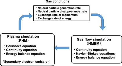
Fig. 3. (Color online) Flow diagram of coupled calculation of plasma and gas flow simulations. 20)
Download figure:
Standard image High-resolution image4. Calculation results
4.1. Calibration of SEE coefficient
Firstly, assuming that there is no SEE, the coupled calculation of plasma and gas flows in simulations was performed at Ar/SF6 = 50/5.0 sccm. As for the Vdc in the Ar/SF6 mixed gas, similarly to the Ar gas described in Sect. 3.2, the Vdc of the lower electrode changed in the range of –772 to –868 V, and the Vdc of the upper electrode became almost constant –667 V. The voltage difference between the upper electrode and the lower electrode was 105–201 V, which was smaller than the average value of each. The calculation result of electron density is shown in Fig. 4. The region where the calculated electron density is low near the upper and lower electrodes corresponds to the sheath region of Ar/SF6 plasma.

Fig. 4. (Color online) Distribution of calculated electron densities assuming no SEE.
Download figure:
Standard image High-resolution imageFrom the results in Fig. 4, we extracted the electron density at the center at the probe position. The probe was set at a height of 23 mm from the lower electrode and the height position corresponded to z = 80 mm in the model shown in Fig. 2. Since r = 0 mm is the center of symmetry of the simulation model and is a singular point, the center position in the simulation was set to r = 2 mm.
The electron density calculated in the simulation was 4.93 × 10¹⁶ m−3, whereas that obtained by experiment was 10.2 × 10¹⁶ m−3. The result shows that the electron density in the simulation was 51.7% lower. We considered that the electron density was low because the effect of SEE was not included. To add the effect of SEE to the simulation, the value of the SEE coefficient γ was increased by 0.01 in the range from 0 to 0.05 and compared with the experimental results. From the results obtained in the simulation, the electron density at (r, z) = (2, 80) was extracted. Figure 5 shows the relationship between the SEE coefficient γ and the electron density. The electron density increased with the increase in γ, and when γ = 0.04, it became 10.26 × 10¹⁶ m−3, which was the closest to the measured electron density. The SEE γ in the Ar/SF6 mixed gas was determined to be 0.04.

Fig. 5. (Color online) Relationship between SEE coefficient and electron density at CNT.
Download figure:
Standard image High-resolution image4.2. Comparison of simulation results with experimental results
The spatial distributions of the experimental and simulation results were compared with those of the SEE coefficient γ = 0.04. Figure 6(a) shows the calculation results of electron density at γ = 0.04. Figure 6(b) shows the electron density distributions along the z-direction at the positions r = 2 (CNT) and r = 35 mm (EDG). The calculated electron density at the probe position (z = 80 mm) was extracted and compared with the experimental results.
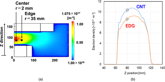
Fig. 6. (Color online) Distribution of calculated electron densities: (a) contour diagram and (b) electron density distributions at absorption probe CNT and EDG.
Download figure:
Standard image High-resolution imageTable IV summarizes the calculated and experimental results. In the table, the experimental and calculation results at γ = 0 are also shown for comparison with those at γ = 0.04. At γ = 0, the electron densities in the simulation for both the center and the edge were lower than those in the experiment. The electron density at the edge to that at the center (EDG/CNT) in the experiment was 83.3% and that in the simulation was 92.70%. On the other hand, the calculation results at γ = 0.04 were close to the experimental results for both the center and the edge. In addition, the EDG/CNT in the experiment was 83.3% and that that in the simulation was 83.3%. By adding the effect of SEE, we found that the spatial distribution of the electron density in the simulation became close to that in the experiment.
Table IV. Results of experiments and coupled calculations of plasma and gas flows in simulations at gas flow rate of Ar/SF6 = 50/5.0 sccm.
| Position | Center | Edge | EDG/CNT [%] |
|---|---|---|---|
| Experiment [×1016 m−3] | 10.20 | 8.50 | 83.3 |
| Simulation without SEE [×1016 m−3] | 4.93 | 4.57 | 92.70 |
| Error [%] | −51.67 | −46.24 | 11.24 |
| Simulation with SEE [×1016 m−3] | 10.26 | 8.55 | 83.33 |
| Error [%] | 0.59 | 0.59 | 0 |
Next, simulation was performed at γ = 0.04 and SF6 flow rate of 2.5 sccm. The electron densities were extracted at the center and edge and compared with the results of the probe measurement. Figure 7 shows the simulation results and probe measurement results. For comparison, the results at SF6 = 5 sccm are also shown. At SF6 = 2.5 sccm, the simulation results at the center and edge were 15.20 × 10¹⁶ and 12.10 × 10¹⁶ m−3, respectively. The calculated electron density at the center was 4.11% higher than the experimental result, and that at the edge was 11.03% lower than the experimental result. It is considered that there is an error of about 10% in the probe measurement and the experimental results and the simulation results are almost in agreement. By setting the SEE coefficient γ at 0.04, we can realize a plasma simulation whose results reproduce the probe measurement result.
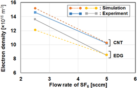
Fig. 7. (Color online) Electron density calculated in simulation and that measured using the absorption probe.
Download figure:
Standard image High-resolution image4.3. Spatial distribution
In Sect. 4.2, the validity of setting the SEE coefficient γ at 0.04 was shown. Therefore, the simulation results at the SEE coefficient γ of 0.04 were investigated. Firstly, the positive and negative charges of the plasma were examined at the center position.
Figure 8(a) shows the densities of electrons and negative ions. The densities of negatively charged particles increased in the order of electrons, SF6 −, and SF5 −, and the total charge was 2.10 × 10¹⁶ m−3. Similarly, Fig. 8(b) shows the densities of positive ions. The densities of positive ions increased in the order of Ar+, SF5 +, and SF2 +. The total charge was 2.24 × 10¹⁶ m−3 and the sum of the densities of negatively charged particles and that of the positively charged ions are almost the same. These results show the validity of the plasma simulation from a viewpoint of charge neutrality in plasmas.

Fig. 8. (Color online) Charged species density calculated in simulation: (a) electrons and negative ions and (b) positive ions.
Download figure:
Standard image High-resolution imageFigures 9(a) and 9(b) respectively show the spatial distributions of the densities of electrons and SF5 −, which are higher than those of other densities in negatively charged particles. In addition, Figs. 9(c) and 9(d) respectively show the spatial distributions of the densities of Ar+ and SF5 +, which are higher than those of other positively charged ions. The electron density is high at the center of the chamber in the height direction, whereas the densities of Ar+, SF5 +, and SF6 − are high near the lower electrode.

Fig. 9. (Color online) Spatial distributions of electron density (a), SF6 − (b), Ar+ (c), and SF5 + (d).
Download figure:
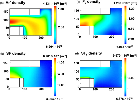
Standard image High-resolution imageFigure 10 shows the spatial distribution of species other than charged particles in the plasma. It shows (a) the Ar* density, (b) the SF density, (c) the F2 density, and (d) the SF5 density. Ar* has been reported to have a long lifetime of more than 10 s. 36) Therefore, it is transported toward the exhaust port by the gas flow and has high density even near the port. In the coupled calculation of plasma and gas flows in simulations, this phenomenon was reproduced as reported in the previous paper. 20)
Fig. 10. (Color online) Spatial distributions of Ar* (a), SF (b), F2 (c), and SF5 (d).
Download figure:
Standard image High-resolution image
5. Discussion and conclusions
Positive ions collide with the electrode and secondary electrons are emitted. The energy received by ions before collision can be approximated by the amount of charge applied with Vdc, as described in Sect. 3.2. The velocity at which cations collide depends on the mass of the ions. Therefore, we estimated the average mass of ions at SF6 = 5.0 sccm and γ =0.04. Using the positive ion density at the center position shown in Fig. 8(b), we calculated the average mass by multiplying the mass of each ion species by the density ratio. As a result, the average mass per mole was determined to be 44.21 g, which is slightly larger than that of Ar, which has a mass of 39.948 g per mole.
So far, we have discussed the results of the coupled calculation of plasma and gas flows in simulations for dual-frequency excited Ar/SF6 plasma. In particular, by focusing on the effect of SEE, we varied the value of its coefficient γ, and γ = 0.04 was determined from the comparison of calculation results with experimental results. The dependence of electron density on spatial distribution and SF6 gas partial pressure was compared between calculation and experimental results at γ=0.04.
As a result, at SF6 = 5.0 sccm, the EDG/CNT from calculation results was the same as that from experimental results, and the spatial distribution of electron density could be reproduced. Furthermore, at SF6 = 2.5 sccm, the error from the experiment including the spatial distribution was in the range of −11.03% to 4.11%. By the coupled calculation of plasma and gas flows in simulations incorporating SEE, we were able to reproduce the spatial distribution and the dependence of electron density on the SF6 partial pressure in a dual-frequency excited Ar/SF6 plasma.
Acknowledgments
This work was carried out by the joint usage/research program of center for Low-temperature Plasma Sciences, Nagoya University.