Microtubules: dynamically unstable stochastic phase-switching polymers

Microtubules are structures formed from the heterodimeric protein tubulin (Fig. 2). Heterodimers are complexes of $\unicode{945}$- and $\unicode{946}$-monomers of tubulin. Linear chains of tubulin molecules called protofilaments are aligned along the generatrix of a hollow cylinder roughly $25\ {\text{nm}}$ in diameter.

Zoom In Zoom Out Reset image size

The bonds between tubulin molecules inside a protofilament are referred to as longitudinal and those between tubulins of neighboring protofilaments as lateral. In a cell, microtubules have a fixed number (13) of protofilaments, whereas the number of protofilaments in growing microtubules varies from 10 to 18 [15, 16]. A microtubule has polarity: the end that terminates with $\unicode{946}$-subunits is called the plus end, and the one terminating with $\unicode{945}$-subunits is the minus end. Remarkably, the plus and minus ends have different characteristics: the former lengthen faster but shorten more slowly than the latter [17–19]. The polarity of microtubules also controls the direction of motion of such proteins as kinesins [20], which move in a highly predetermined direction along microtubules due to the use of the energy of adenosine triphosphate (ATP) hydrolysis.

Another interesting structural property of microtubules is helicity. Protofilaments are generally arranged such that there is a helical shift of three monomers between the adjacent protofilaments winding around the microtubule axis (Fig. 2). Most side surfaces of protofilaments are bound laterally such that $\unicode{945}$-monomers of one protofilament interact with $\unicode{945}$-monomers of the adjacent one, while $\unicode{946}$-monomers of two neighboring protofilaments interact with each other. However, the odd pitch of the helix results in the formation of a so-called seam between a pair of protofilaments, i.e., a region of the microtubule lattice where lateral interaction between $\unicode{945}$- and $\unicode{946}$-monomers takes place [21]. The molecular peculiarities of the seam, if any, and their possible role in the functioning of microtubules remain to be elucidated.

The process of microtubule growth is a sequence of random attachments of new tubulin molecules to the end of any protofilament, as is confirmed by results of cryoelectron microscopy [22, 23], suggesting that the tips of growing microtubules adopt a straight shape [24–26].

Images of the ends of disassembling microtubules show that terminal dimers curl to form a ring before they dissociate [24–26]. It was concluded that longitudinal bonds are stronger than lateral ones, which explains why disassembly starts from the rapid breakdown of lateral bonds, while longitudinal bonds break later. In this case, rather big protofilament fragments peel away from the microtubule, which accounts for the depolymerization rate being much higher than the growth rate.

It was mentioned in the Introduction that the growth of microtubules occurs as a series of stochastic transitions from the slow lengthening phase to the rapid depolymerization phase and back [27]. Catastrophes and rescues are readily seen in Fig. 3, exemplifying single microtubule dynamics.

Zoom In Zoom Out Reset image size

Generally speaking, any reversible polymerization process is characterized by growth rate fluctuations. Sometimes, they are so pronounced that they may lead to the shortening of a polymer. Could the observed catastrophes and rescues be such thermal fluctuations? Figure 3b presents the results of calculations in the framework of a molecular dynamics models taking thermal fluctuations into account as described below [28]. The figure illustrates the case where tubulins attach and detach one after another as during the polymerization of a single-chain polymer. Evidently, growth fluctuations do exist, but their amplitude is much smaller than the shrinkage after a catastrophe.

A microtubule grows as tubulin dimers sequentially attach to its end. Each monomeric tubulin in a dimer is bound to a guanosine triphosphate (GTP) molecule. Soon after the dimer attaches to a microtubule, the GTP molecule bound to the $\unicode{946}$-monomer undergoes hydrolysis and is converted into a guanosine diphosphate (GDP) molecule [29, 30], whereas the GTP molecule bound to the $\unicode{945}$-monomer is never hydrolyzed [31]. However, dimers in a solution barely hydrolyze GTP [32]. GTP hydrolysis is accompanied by release of a large amount of chemical energy, which appears to be responsible for microtubule 'destabilization', making the system thermodynamically unstable.

According to the modern concept, the molecular mechanism responsible for the ability of microtubules to switch from time to time between slow growth and rapid depolymerization phases is related to the storage of the energy released in GTP hydrolysis in the form of strained conformation of tubulin monomers inside the tubule body. A microtubule grows as GTP-bound tubulin dimers, straightened in the solution, attach one after another to its end. Protein conformation in the dimer changes after the attachment, which causes GTP hydrolysis and release of the chemical energy of GTP molecules. It is believed that this energy is not dissipated into heat but is used to alter the equilibrium conformation of the GDP–tubulin complex [6]. However, the molecule bound to its neighbors in the tubule wall cannot relax into a new conformation. This means that new dimers in the same (GTP) conformation continue to attach to the end of the growing microtubule, while almost all of its body, starting from a certain distance from the end, consists of molecules of different conformations (GDP). Due to this, the largest part of the microtubule is mechanically strained and unstable.

Owing to continuous attachment of GTP dimers to the end of a microtubule, it always contains some number of dimers that have not yet hydrolyzed the GTP molecule. Such a part, rich in GTP dimers, is called the GTP cap (Fig. 3c). It encircles the microtubule tip and thereby prevents relaxation of the majority of the dimers that have already passed into the strained state; in this way, the microtubule is protected from disassembly.

The detailed mechanism of the GTP cap action is a matter of controversy. According to the classical model, GTP-bound tubulin dimers stabilize microtubules, because longitudinally linked GTP dimers tend to form a straight linear chain, whereas GDP dimers find it energetically favorable to bend into a horn-like structure with a curvature radius around $20\ {\text{nm}}$ [26, 33–35]. An alternative hypothesis assumes that both tubulin complexes (with GTP and GDT) have a roughly identical curved conformation, and tubule stabilization by GTP dimers is due to lateral bonds between them, which are stronger than those between GDP dimers [36].

This implies the undeniably important role of GTP hydrolysis and the accompanying conformational changes in tubulin molecules [37]. Indeed, microtubules undergoing polymerization in the presence of an unhydrolyzable GTP analog grow continuously and do not experience catastrophes [38]. In contrast, microtubules composed of GDP dimers are highly unstable and prone to disassembly. This inference is confirmed by results of experiments on cutting microtubules by a focused UV radiation or a thin needle [33, 39]. In these experiments, microtubules with cut terminal layers immediately underwent disassembly, starting from the plus end.

To date, neither the constant nor the mechanism of GTP hydrolysis have been reliably determined. For this reason, the scientific community has not yet reached a consensus regarding the number of GTP dimers on a growing microtubule end; the estimates vary from one to a few dozen layers. The following data appear to support arguments in favor of a small size of the GTP cap.

First, earlier attempts to detect GTP tubulin in microtubules by biochemical methods failed, giving reason to suppose that the number of GTP tubulins inside a microtubule is very small, below the method detection limit [40, 41].

Second, Refs [42, 43] report experiments in which microtubules were polymerized at different tubulin concentrations, after which free tubulin was sharply diluted in order to see how soon the microtubules begin to disassemble. The authors hypothesized that if the number of GTP subunits increases with concentration, then the time before the transition to disassembly must increase proportionally after free tubulin dilution. However, this assumption proved to be invalid, which was interpreted as evidence that the GTP cap always has the same small size. It fairly well accounts for a weak dependence of the catastrophe rate on the tubulin concentration in solution [44]. Moreover, experiments with an unhydrolyzable GTP analog showed that a single GTP layer is sufficient to stabilize a microtubule and thereby prevent its disassembly [45, 46].

Nevertheless, results of certain experiments suggest that GTP caps may have more than one layer. First, the end of a growing microtubule frequently shortens locally by more than $40\ {\text{nm}}$ (5 layers) in the absence of a catastrophe [47]. Second, the end-binding protein-1 (EB1) appears to selectively interact with GTP tubulins within a microtubule [48] by virtue of its ability to recognize a segment as long as a few dozen of layers at the end of the microtubule [49]. The size of the GTP cap identified by EB1 increases with increasing the microtubule growth rate in the presence of increased tubulin concentration, in conflict with the model of an invariably monolayer GTP cap.

Time dependences of the catastrophe rate deduced from in vitro experiments suggest that the probability of the microtubule transition from slow growth to rapid disassembly increases with time [50, 51]. In other words, 'younger' microtubules are less likely to undergo a catastrophe than 'older' ones (Fig. 4).

Zoom In Zoom Out Reset image size

The phenomenon of catastrophe frequency growth with time is termed 'aging'. A delayed onset of catastrophes in young microtubules suggests a multi-stage character of this process. As is known, the differential distribution of the times of single-stage events obeys an exponential law, whereas the nonexponential form of the distribution implies a multi-stage process [52]. It was shown in experiments that the distribution of microtubule lifetimes has the form described by the gamma distribution [50]. This means that a microtubule has to pass through a few consecutive stages before it experiences a catastrophe. The longer the microtubule 'lives', the more advanced stage it reaches and the higher is the probability of its disassembly. If this were a single-stage process, there would be no delay of catastrophe for a microtubule starting to grow, and the time dependence of the catastrophe rate would be constant (see the horizontal straight line in Fig. 4) [51]. It remains unclear what the multiple events leading to a catastrophe are. It was thought that a growing microtubule experiences the influence of certain destabilizing defects [51, 53]. Once formed, such defects persist and accumulation of three of them leads to a catastrophe. According to an alternative hypothesis, a defect may correspond to the spontaneously arising inability of a single protofilament to bind tubulin (Fig. 5a). One more variant of a destabilizing event is sequential changes in the growing microtubule tip structure [54]. In this case, the microtubule tip sharpens as it grows due to the increasing difference between the lengths of individual protofilaments; as soon as sharpening becomes critical, a catastrophe occurs (Fig. 5b).

Zoom In Zoom Out Reset image size

Neither calculations in the framework of multiple-protofilament models nor experimental data in support of the hypothesis of three irreversible destabilizing defects are presented in Refs [51, 53]. At the same time, the results of numerical simulation and experimental evaluation of the sharpening of microtubule tips by fluorescent and electron microscopy presented in [54] seem consistent with the alternative hypothesis of sequential changes in the growing tips. However, they were not confirmed in later studies (see, e.g., [55]). Moreover, the statistical analysis of experimental data in Ref [56] failed to demonstrate a significant monotonic increase in the degree of sharpening with time [28].

A catastrophe changes the structure of the microtubule tip: its roughly cylindrical shape turns into a throat-like one with protofilaments extended radially outwards (Fig. 3c). It was shown recently that such a change is of utmost importance because it enables the depolymerizing microtubule to function as a molecular motor exerting force. In vitro experiments made it possible to directly observe how radially extended protofilaments of a microtubule push microspheres attached to their wall [57]. The pushing force was measured by optical tweezers (a focused laser beam pulling and trapping wavelength-sized dielectric particles) (Fig. 6a). Because the force generated by one or two protofilaments of a disassembling microtubule is applied to the surface of a microsphere, the equilibrium condition is the equality of the moments of forces of the microtubule and the tweezers:

$$\begin{equation} F_{\text{opt}}R=F_{\text{MT}}l\,. \end{equation} \tag{ 1 }$$

Here, $F_{\text{opt}}$ is the optical force being measured that tends to bring the microsphere back to the center of the trap, $R$ is the arm of this force equal to the microsphere radius $(250\ {\text{nm}}), F_{\text{MT}}$ is the force generated by the depolymerizing microtubule, and $l$ is the arm of the force $F_{\text{MT}}$, roughly equal to the deviation of a curved protofilament from the microtubule wall $(\approx 20\ {\text{nm}})$. The arm of the microtubule force being roughly $10\ {\text{times}}$ that of the optical force, the force signal measured by the optical tweezers is relatively weak. However, the pushing force of a protofilament is around $2.5{-}5\ {\text{pN}}$ once the ratio of the arms is taken into account.

Zoom In Zoom Out Reset image size

Another series of experiments with an altered measurement configuration was designed to determine the force generated by the entire microtubule as opposed to individual protofilaments under imitated intracellular conditions [13]. For this, a microsphere attached to a protein ring of the Dam1 complex with artificially formed protein linkers was suspended from the microtubule (Fig. 6b). It is supposed that microtubules are similarly attached to a chromosome in yeast cells, where the role of the ring is played by the same Dam1 protein complex and linkers are proteins of the NDC80 complex [58]. Such alteration of the measurement configuration resulted in a multifold increase in the registered force signal.

Measurements reported in Ref. [13] allowed estimating the force generated by a microtubule as $30\ {\text{pN}}$ with the nonideality of the coupling device in the form of the Dam1 ring taken into account (efficiency coefficient $\sim 40{-}50\hbox{%}$). This force is rather strong on the cellular scale, being many times the maximum force generated by motor proteins kinesin ($\sim 7\ {\text{pN}}$ [59]) and dynein ($\sim 1\!-\!7\ {\text{pN}}$ [60, 61]) responsible for the transfer of many intracellular components over microtubules.

It can be speculated based on the above findings that microtubules are the main sources of mechanical work needed to move chromosomes. This assumption is confirmed by experiments in which elimination of minus-terminal motor proteins from yeast cells did not change the speed of chromosome movement in mitosis, most likely entirely due to the microtubule depolymerization [62, 63].

To conclude, there is a wealth of experimental data on the dynamic, structural, and mechanical properties of microtubules that must be taken into consideration in the elaboration of theoretical models of their dynamically unstable behavior. The most important experimental findings include (1) structural data on the shape of the tips of growing and disassembling microtubules, (2) dependences of growth and disassembly rates on tubulin concentrations in a solution, (3) data on microtubule disassembly after a sharp dilution of free tubulin, (4) the distribution of microtubule polymerization times, the so-called microtubule aging phenomenon, and (5) the ability of depolymerizing microtubules to develop a significant force.

Traditionally, the method of molecular dynamics calculations is the most detailed method for describing the evolution of a system of chemically interacting particles, because it explicitly takes thermal fluctuations into account but considers chemical reactions as separate physical interactions. Because the reactions are results of random collisions of diffusing molecules, the evolution of a system of interacting particles is a stochastic rather than deterministic process.

Stochasticity at the level of collisions between individual molecules is frequently ignored, for example, in chemical kinetics; instead, a deterministic change in the number and concentration of reactant molecules is considered. In this case, the main equation describing chemical transformations is the law of mass action, the system of differential equations of the form

$$\begin{equation} {{\text{d}} X_1\over {\text{d}} t}=f_1(X_1,\ldots,X_N),\quad i=1, \ldots, N\,, \end{equation} \tag{ 2 }$$

where $X_1$ is the number of molecules of the $i$th substance from the totality of reactants $S_i$ $(i=1, \ldots, N\,)$, and $f_1$ are functions depending on the specificity of the reactants.

Once the number of reacting molecules of at least one of the components is sufficiently small, stochasticity may greatly contribute to the process. New dimers attach to the end of a microtubule; therefore, the number of dimers in the microtubule interacting with those diffusing in the solution is only 13, which means that neither stochasticity nor consideration of separate interactions can be ignored [89]. In what follows, we describe methods by which the microtubule dynamics are simulated at the level of separate interactions.

One of the most popular algorithms for microtubule simulation is the kinetic Monte Carlo method. To give an insight into this method, we consider a well-stirred system of $N$ molecules of different reactants $\{S_1,\ldots, S_N\}$ that interact via $M$ reactions $\{R_1,\ldots,R_M\}$. Let the system be placed in a certain fixed volume ${\it{\Omega}}$ at constant temperature. We further let $X_i(t)$ denote the number of molecules of substance $S_i$ at time $t$. The aim is to describe the vector of state ${\bf X}(t)=(X_i(t),\ldots, X_N(t))$ at each time instant, knowing the state vector at the initial instant ${\bf X}(t_0)\equiv {\bf x}_0$.

Each set of reactions can be characterized by two quantities. One is ${\bf \nu}_j\equiv (\nu_{1j},\ldots, \nu_{Mj})$, where $\nu_{i\,j}$ is the increment in the number of $S_i$ molecules resulting from the reaction $R_j$. In other words, if the system is in a state ${\bf x}$, it passes into state the ${\bf x}+{\bf \nu}_j$ after the reaction $R_j$ is completed. The other quantity characterizing the reaction $R_j$ is the probability per unit time $a_j$, i.e.,

$$\begin{equation} \begin{aligned} &a_j({\bf x}){\text{d}} t\ is\ the\ probability\ that\ in\ the\ state\ {\bf X}(t)={\bf x}\ the\\ & reaction\ occurs\ within\ an\ infinitesimal\ time\ interval\\ &[t, t+{\text{d}} t\,]. \end{aligned} \end{equation} \tag{ 3 }$$

The physical meaning of $a _j({\bf x})$ can be explained as follows. For an $S_1\to \ldots \,$ type reaction involving a single substance, there is a constant $c_j$ such that $c_j{\text{d}} t$ is the probability of a transformation of $S_1$ at the next infinitesimal time step ${\text{d}} t$. If the reaction mixture contains $x_1$ of $S_1$ molecules, the probability of one of them reacting during the next time interval ${\text{d}} t$ is $x_1 c_j {\text{d}} t$. Therefore, $a_j({\bf x})=x_1c_j$.

In the presence of two interacting substances and the reaction $R_j$ has the form $S_1+S_2\to \ldots \,$, then there is a constant $c_j$ such that $x_1x_2 c_j{\text{d}} t$ is the probability of reaction of a certain pair of molecules, $S_1\!-\!S_2$, within a time interval ${\text{d}}t$, where $x_1$ and $x_2$ are the numbers of $S_1$ and $S_2$ molecules. Then $a_j({\bf x})=x_1x_2 c_j$. In this case, the quantity $c_j$ for the reaction $S_1\to \ldots$ is numerically equal to the reaction constant $k_j$, while in the case of different reactants $S_1+S_2\to \ldots, c_j=k_j/{\it{\Omega}}$ [87, 89–91]. For molecules of the same type, $c_j=2k_j/{\it{\Omega}}$.

We are interested in the conditional probability of the system transition into a state ${\bf X}(t)={\bf x}$ from a state ${\bf X}(t_0)={\bf x}_0$. In the Monte Carlo method, stochastic trajectories ${\bf X}(t)$ are found in numerical form instead of finding the probability density function $F_{{\bf X}(t)}$ analytically. For this, the probability function is used:

$$\begin{equation} \begin{aligned} &p(\tau, \,j\,|{\bf x}, t){\text{d}} t\ is\ the\ probability\ that\ in\ a\ state\ {\bf X}(t)={\bf x},\\ &the\ reaction\ occurs\ within\ an\ infinitesimal\ time\ interval\\ &[t+\tau,\, t+\tau+\!{\text{d}} \tau]. \end{aligned} \end{equation} \tag{ 4 }$$

The exact formula for $p(\tau,\,j\,|{\bf x}, t)$ has the form [87, 91]

$$\begin{equation} p(\tau,\,j\,|{\bf x}, t)=a_j({\bf x})\,\exp{(-a_0({\bf x})\,\tau \big)}\,, \end{equation} \tag{ 5 }$$

where

$$\begin{equation} a_0({\bf x})=\sum^M_{j^{\;\prime}=1} a_{j^{\,\prime}}({\bf x})\,. \end{equation} \tag{ 6 }$$

Equation (5) provides a mathematical basis for simulation using stochastic chemical kinetics. In (5), $\tau$ is an exponentially distributed random quantity with the mean equal to the standard deviation, $1/a_0({\bf x})$, with $j$ being the statistically independent random integer variable with the conventional probability $a_j({\bf x})/a_0({\bf x})$ (in fact, the weight of a single event).

The following variables are used to describe microtubule evolution: the parameter $j=1, 2, 3$ is one of the three events (attachment, detachment, or GTP hydrolysis) and $a_j({\bf x})\equiv k_j$ is the characteristic onset time of each of the possible events. The numerical method for finding the stochastic trajectory ${\bf X}(t)$ of microtubule evolution is based on Eqn (5). The simulation procedure is as follows:

• (1)  
  initialization of time $t=t_0$ and the initial state of the system ${\bf x}={\bf x}_0$;
• (2)  
  for each $i$th monomer and possible $j$th elementary event, a random quantity $r_{i\,j}$ uniformly distributed over an interval from 0 to 1 is generated;
• (3)  
  all times for each elementary event are found:

  $$\begin{equation} t_{i\,j}=-{\ln {(1-r_{i\,j})}\over k_{i\,j}}; \end{equation} \tag{ 7 }$$
• (4)  
  the event corresponding to the shortest time $t_{i\,j}$ is assumed to have occurred;
• (5)  
  the system configuration is updated in accordance with the selected event and the time is shifted as $t\rightarrow t+t_{i\,j}$;
• (6)  
  steps 2–5 are repeated.

This approach to the description of microtubule dynamics was applied in the work by Chen and Hill [14, 64, 92]. In the model in [64], dating back to 1985, a microtubule is represented by a helix of 13 protofilaments with a five-subunit shift along the seam. In this model, subunits can build into or dissociate from the microtubule only as separate dimers, regardless of the breakdown of lateral or longitudinal bonds during dissociation (Fig. 7a). Nor can dimers be present at the end of the microtubule in the absence of a longitudinal neighbor and at least one lateral one. The model uses the random hydrolysis rule, which means that GTP hydrolysis occurs with a certain probability at any site of the microtubule, both in the terminal layer of dimers and in a gel. Although the model allows considering individual probabilities of the GTP–GDP transition depending on the dimer position, the constants for this transition are chosen to be identical over the entire microtubule length.

Such a simple approach was used to reproduce transitions between growth and shrinkage states and to describe the dependence of the averaged tubulin polymerization rate on its concentration in the solution known at that time. But the data on individual microtubule dynamics were unavailable and the model disregarded them.

To describe results of new experiments, e.g., the recently discovered weak dependence of the time of microtubule transition to depolymerization after dilution of free tubulin, Bayley and coauthors proposed a different model with the induced hydrolysis rule in which GTP tubulins are located strictly in the terminal layer, regardless of the free tubulin concentration (Fig. 7b) [65, 66, 69]. This model correctly described dilution experiments and the weak dependence of the microtubule catastrophe rate on tubulin concentration.

But the above kinetic models had a common drawback: they did not consider conformation of the tubule end and therefore could not describe structural data corresponding to different phases of the microtubule growth. An attempt to qualitatively consider the microtubule end configuration was undertaken by VanBuren et al. in 2002 [74] (Fig. 7c). It was an important step forward in comparison with preceding models and became a transient stage toward subsequent mechanistic approaches to the description of microtubule dynamics. This model is in excellent agreement with the modern concept of the microtubule lattice as a B-type lattice, i.e., a left-handed three-start helix, suggesting that a single longitudinal bond is enough to enable tubulin molecules to attach to a microtubule.

In this model, each bond corresponds to an energy depending on the nucleotide composition of interacting dimers. In other words, the probability of dimer dissociation depends on whether the nucleotide to which it is bound is hydrolyzed and on the number of newly formed bonds.

The authors of Ref. [74] were the first to try to consider the influence of curling oligomers at the end of a microtubule on dynamic instability under the assumption that the formation of an outwardly extending throat at the tubule tip is indispensable for maintaining the disassembly phase. Because a rapidly disassembling microtubule carries curling oligomers on its end, the GTP dimers attached to them no longer act as stabilizers unable to form lateral bonds. To take this fact into account in the framework of a kinetic model, an artificial rule was introduced to distinguish between 'curled' and 'uncurled' tubulin oligomers.

In 2012, to further modify the description of a microtubule, Margolin et al. [80] considered separate breaks of lateral and longitudinal bonds (Fig. 7d). In the framework of artificially introduced rules, they restricted the alternation of bond-breaking and bond-forming processes to those proceeding consecutively 'from top down' and 'from bottom up', respectively. To imitate the stabilizing action of adjacent protofilaments, the authors introduced a coefficient decreasing the probability of breakdown of a lateral bond in the presence of lateral bonds in neighboring protofilaments. These rules allow taking the differences in the structure of growing and shortening ends of microtubules into account more comprehensively than in earlier models. A unique result in Ref. [80] was the prediction of interprotofilament 'cracks' in the microtubule body. The cracks at the ends of both growing and shrinking microtubules caused their destabilization. Specifically, the probability of catastrophes increased with increasing the number of cracks.

Another important model describing microtubules with the help of the kinetic Monte Carlo method was proposed by Van Buren et al. in 2005 [75] and used later in Ref. [54]. Its fundamental difference from the preceding models was an attempt to include the interactions inside the microtubule based on the energy potentials influencing the probability of breakdowns of dimer–dimer bonds. On these grounds, the model in [75] is regarded as a molecular-mechanokinetic one.

Geometrically, a microtubule is represented as a cylinder, and protofilaments are described as a chain of connected vectors, with the beginning and the end of each vector being two longitudinal binding sites of the respective monomer (Fig. 8).

Zoom In Zoom Out Reset image size

Each monomer is described by three parameters: two rotation angles $\varphi$ and $\theta$ and the length $D$. The angles $\theta$ and $\varphi$ determine the equilibrium bending stress-free direction of the monomer vector. The angle $\theta$ corresponds to outward bending of protofilaments, such that $\theta=22^{\circ}$ for GDP dimers curling at the end of the microtubule and $\theta=0$ for straight GTP protofilaments. The equilibrium angle is equal to zero for both states. The deviation of the current vector position from equilibrium is described by a quadratic potential. The quantity $D$ is the sum of the monomer length $(4\ {\text{nm}})$ and extension along the protofilament $d$. The interaction between monomers in adjacent protofilaments is described by the distance between lateral interaction sites $S$, which is calculated given the coordinates $\{\varphi, \theta, D\}$. Extensions $d$ and $S$ are described by Hookean potentials with a break upon achievement of the maximum interaction energy. The current monomer vector deflects from the equilibrium one by the angle ${\it{\Phi}}$. The energy potential is also quadratic in ${\it{\Phi}}$. The energy minimization algorithm is used to find coordinates $\{\varphi, \theta, D\}$ near the end of the microtubule.

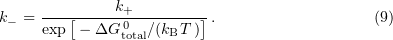
This model involves a quasiequilibrium approximation, which means that the microtubule is considered to be an equilibrium system at any time instant. The equilibrium constant is represented in the form

$$\begin{equation} K={k_+\over k_-}=\exp\bigg(-{\Delta G_{\text{total}}^{\,0}\over k_{\text{B}}T}\bigg)\,, \end{equation} \tag{ 8 }$$

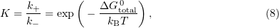
where $k_+$ is the attachment reaction constant expressed in units $[{\text{M}}^{-1}\ {\text{s}}^{-1}], k_+$ is the detachment constant, $\Delta G_{\text{total}}^{\,0}$ is the overall change in the binding free energy for a given dimer, and $k_{\text{B}}$ is the Boltzmann constant. Hence, the calculated probability of dissociation is

$$\begin{equation} k_-={k_+\over \exp{\big[-\Delta G^{\,0}_{\text{total}}/(k_{\text{B}}T\,)\big]}}\,. \end{equation} \tag{ 9 }$$

When the sum of binding and strain energies for a given bond is greater than or equal to zero, the bond is considered broken.

With the energy and dissociation constants being found, the kinetic Monte Carlo algorithm is used as described above. The list of possible events realized with the help of the Monte Carlo method includes bond breakage and GTP hydrolysis. After each new event is accepted, the Monte Carlo method is supplemented by the procedure for finding a local energy minimum of the system [93], and all the preceding steps are repeated.

In the approach used by Van Buren and coauthors, microtubule geometry and its influence on the probability of bond breakage were taken into account because the probability of dissociation depends on both the bond number and stress, as well as on the nucleotide base composition of the bonds. However, this microtubule model is not free from shortcomings, despite its progressive character. For example, the form of potentials is described by a nonsmooth function with a singularity at the bond breakage point; at this point, the energy gradient decreases abruptly from the maximum value to zero. More importantly, the described mechanokinetic approach disregards thermal fluctuations that may play a key role in microtubule dynamics.

3.3.1. Static models.

In early studies [93, 94] reporting on detailed analyses of the mechanical properties of microtubules, the microtubule surface was modeled in the form of a two-dimensional homogeneous anisotropic material with two orthogonal inner curvatures. One tended to bend the surface outward, the other to roll it into a cylinder. The main result in Refs [93, 94] was the computed shape of the end of a microtubule corresponding to the minimal energy of such a sheet. The resulting shape, called a 'structural cap', provided a basis for postulating a different dynamic behavior of the microtubule. However, the abstract description of microtubules as a two-dimensional material was not based on real structural data, which strongly limited the interpretation of the results obtained with this model. As mentioned above, the mechanical description of a microtubule requires a more detailed consideration at the molecular level.

Molodtsov and coauthors were the first to undertake mechanistic microtubule modeling at the molecular level [12, 71]. A microtubule was simulated as a left-handed helical structure with a pitch of three monomers. The elementary subunit of the model is a tubulin dimer having two lateral bonds with dimers of neighboring protofilaments and one longitudinal bond with dimers along the protofilament. Lateral interactions are described by continuously differentiable inter-dimer interaction potentials having virtually the same shape as protein–protein interaction potentials [95] (Fig. 9a). The longitudinal potentials of this model have no discontinuities. The bending potentials inside protofilaments are assumed to be quadratic:

$$\begin{equation} g_{k,\,n}^{{\text{bending}}}(\chi_{k,\,n})={1\over 2}\,B(\chi_{k,\,n}-\chi_0)^2\,, \end{equation} \tag{ 10 }$$

$$\begin{equation} \chi_0=\chi^{\,\text D}_0\quad{\text{or}}\quad\chi^{{\text{T}}}_0\,. \end{equation} \tag{ 11 }$$

Here, $B$ is the parameter characterizing the rigidity of longitudinal bonds assumed to be similar for the T- and D-forms of tubulin, and $\chi_{k,\,n}=\theta_{k,\,n}-\theta_{k-1,\,n}$ is the angle of deflection of the $k$th and $(k-1)$th subunits from each other in the $n$th protofilament.

Zoom In Zoom Out Reset image size

Bending of each protofilament is limited by a plane (Fig. 9b). The equilibrium angle $\chi_0$ can be found from structural data [34]. For GDP tubulin, $\chi^{\,\text D}_0\approx 0.2$ for each monomer, whereas GTP dimers tend to form straight configurations [26, 96]. The bending energy $G_n$ of the $n$th protofilament is represented as the sum

$$\begin{equation} G_n=\sum_k g^{{\text{bending}}}_{k,\,n}(\chi_{k,\,n})\,. \end{equation} \tag{ 12 }$$

To describe lateral bond breakage, the potential

$$\begin{equation} V_{k,\,n}(r_{k,\,n})=A\bigg({r_{k,\,n}\over r_0}\bigg)^2\exp\bigg(\!-{r_{k,\,n}\over r_0}\bigg)\, \end{equation} \tag{ 13 }$$

was used [95], where $r_0$ and $A$ are parameters characterizing the length and the binding energy.

Thus, the total potential energy of a microtubule is the sum of longitudinal and transverse interactions of all the points involved, including (1) the sum of potential energies of longitudinal (flexural) interactions between subunits inside a protofilament and (2) the sum of interactions among all lateral contacts in adjacent protofilaments.

The very low microtubule energy facilitated the search for and analysis of local energy minima of the system by the conjugate gradient method and thereby allowed estimating the microtubule stability depending on the size of the GTP cap and other parameters of the model. However, it was impossible to simulate microtubule dynamics.

3.3.2. Metropolis pseudodynamics method.

The Molodtsov model [71] was soon supplemented by the Metropolis algorithm as proposed in [70]. The Metropolis algorithm is a modified Monte Carlo method for describing the tubulin subunit dynamics in a microtubule [70].

The Metropolis algorithm [97] is frequently used to describe the evolution of multi-molecular systems in a potential electric field. The algorithm can be represented as follows. We consider a system of $N$ particles with the potential energy

$$\begin{equation} E={1\over 2}\,\sum^N_{i=1}\sum^N_{j=1} V(d_{i\,j})\,,\quad i\ne j\,, \end{equation} \tag{ 14 }$$

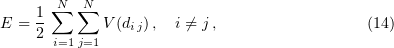
where $V$ is the potential energy between molecules and $d_{i\,j}$ is the maximum separation between particles $i$ and $j$. To calculate the equilibrium value of a certain characteristic $F$ of the system, the formula for a canonical ensemble is used,

$$\begin{equation} \bar{F}={\int F\exp\big[-E/(k_{\text{B}}T\,)\big]{\text{d}}^{2N}p{\text{d}}^{2N}q\over \int \exp\big[-E/(k_{\text{B}}T\,)\big]{\text{d}}^{2N}p{\text{d}}^{2N}q}\,, \end{equation} \tag{ 15 }$$

where $\!{\text{d}}^{2N}p{\text{d}}^{2N}q$ is the volume element in the $2N$-dimensional configuration space. Because this integral is frequently impossible to calculate numerically, the approximate Monte Carlo method is used, in which integration is performed over a random sample of points rather than the total set of them. In other words, an arbitrary position of $N$ particles inside the system is chosen (i.e., a random point in the $2N$-dimensional configuration space). Then the system energy is computed from formula (14), and the statistical weight $\exp{[-E/(k_{\text{B}}T\,)]}$ is assigned to a given configuration.

The statistical weight of random configurations in densely packed systems is frequently very small because the quantity $\exp{[-E/(k_{\text{B}}T\,)]}$ is very small with high probability. In [98], Metropolis et al., instead of choosing arbitrary configurations and assigning the weight $\exp{[-E/(k_{\text{B}}T\,)]}$ to them, proposed choosing configurations with the probability $\exp{[-E/(k_{\text{B}}T\,)]}$ and assigning an equal weight to them. In this case, all particles are shifted from the initial configuration by the rule

$$\begin{equation} \begin{aligned} &X\to X+\alpha\xi_1\,,\cr &Y\to Y+\alpha \xi _2\,, \end{aligned} \end{equation} \tag{ 16 }$$

where $\alpha$ is the maximum allowable displacement and $\xi _1$ and $\xi _2$ are uniformly distributed random numbers from the interval $(-1, 1)$. The energy changes due to the shift, $\Delta E$, are then calculated. If $\Delta E < 0$, i.e., the displacement decreased the energy, the configuration is accepted. If $\Delta E>0$, the displacement is accepted with the probability $\exp{[-\Delta E/(k_{\text{B}}T\,)]}$. Every time, a newly generated number $\xi _3$ is taken from the interval (0, 1): if $\xi _3< \exp{[-\Delta E/(k_{\text{B}}T\,)]}$, the system passes into a new state; if $\xi _3>\exp{[-\Delta E/(k_{\text{B}}T\,)]}$, the system reverts to the previous state. The system is considered to have passed to a new state irrespective of whether the displacement is accepted. Therefore,

$$\begin{equation} \bar{F}={1\over M}\,\sum^M_{j=1} F_j\,, \end{equation} \tag{ 17 }$$

where $F_j$ is the value of $F$ at the $j$th step.

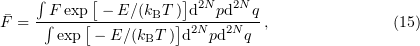
Using ergodicity, it can be shown that the method in question chooses configurations with the probability $\exp{[-E/(k_{\text{B}}T\,)]}$. Let $v_r$ be the number of systems of the ensemble in a state $r$. It can be proved that after a large enough number of steps, the ensemble tends to the distribution of the number of molecules by energy states given by

$$\begin{equation} v_r\sim \exp\bigg(\!-{E_r\over k_{\text{B}}T}\bigg)\,. \end{equation} \tag{ 18 }$$

We suppose that the systems of the ensemble made a step and let $P_{rs}, P_{rs}=P_{sr}$ (with $\xi_l$ being distributed uniformly) denote the probability that this step (whether accepted or not) resulted in the transition from the state $s$ to the state $r$. We also suppose that $E_r>E_s$. Then the number of systems passing from the state $r$ to the state $s$ is $v_rP_{rs}$, because transitions to states with a lower energy are allowed. The number of systems making backward transitions in the configuration space is

$$\begin{equation} N_{\text{f}}=v_sP_{sr}\exp\bigg(\!\!-{E_r-E_s\over k_{\text{B}}T}\bigg)\,. \end{equation} \tag{ 19 }$$

The total number of systems that passed from the state $s$ to the state $r$ is

$$\begin{equation} N_{\text{b}}=P_{rs}\bigg[v_s\exp\bigg(\!\!-{E_r-E_s\over k_{\text{B}}T}\bigg)-v_r\bigg]\,. \end{equation} \tag{ 20 }$$

Hence, for any two states $s$ and $r$, if

$$\begin{equation} {v _r\over v _s}>\exp\bigg(\!\!-{E_r-E_s\over k_{\text{B}}T}\bigg)\,, \end{equation} \tag{ 21 }$$

then a greater number of systems pass on average from the state $r$ to the state $s$. Because the system is ergodic, a single- or multi-step transition from one position to any other position is possible. In other words, after a sufficiently large number of steps, the ensemble must be described in terms of the canonical distribution. Hence, if the transition fails, the old configuration is regarded as newly realized; this gives a greater statistical weight to states with a lower energy.

In 2007, the use of the Metropolis method enabled Efremov et al. [70] to describe the microtubule disassembly as a result of lateral bond breakage under the effect of thermal fluctuations and internal stress in the microtubule lattice. A disassembling microtubule does work to move chromosomes. Due to this, the description of depolymerization in a model containing interaction potentials in the explicit form allowed considering interactions between microtubules and moving chromosomes. However, this model still disregards the attachment of dimers from the solution and GTP hydrolysis, and it does not therefore describe the dynamic instability of microtubules. Moreover, the breakdown of longitudinal bonds at the ends of protofilaments is introduced artificially to maintain the given mean length of curved protofilaments at microtubule ends.

3.3.3. Brownian dynamics and microtubule modeling.

There is an alternative method to describe the dynamics of interacting protein-size particles: the Brownian dynamics simulation technique based on the solution of the equations of motion within certain approximations (see below). It has been shown that in the limit as the coordinate increment tends to zero (i.e., the time step tends to zero), the Metropolis method, including its later realization [99], is equivalent to the Brownian dynamics method [100, 101]. However, transitions between sequential system states in the former technique are not coordinated with time; therefore, it requires an additional time scale calibration with the use of one experimental dependence as a reference one. The Brownian dynamics method does not require such additional calibration.

The use of the Brownian dynamics algorithm in microtubule modeling has become possible with the advent of high-performance computing techniques and powerful supercomputers. We consider this method in greater detail. We write the Langevin equation

$$\begin{equation} m\,{{\text{d}}^{\,2}q\over {\text{d}} t^{\,2}}=-\gamma\,{{\text{d}} q\over {\text{d}} t}+F(t)+F_{\text{rand}}(t)\,, \end{equation} \tag{ 22 }$$

where $m$ is the particle mass, $\gamma$ is the viscosity coefficient of the Brownian particle, $q$ is its coordinate, $F_{\text{rand}}(t)$ is a random force, and $F(t)=-\!{\text{d}} U/\!{\text{d}} q$ is a systematic force acting on the particle in an energy field $U$.

The random force has the following properties:

• (1)  
  averaged over the particle ensemble, the random force is equal to zero (balanced fluctuations), $\langle F_{\text{rand}}(t)\rangle=0$;
• (2)  
  for time intervals longer than the duration of a collision, the random force is uncorrelated, $\langle F_{\text{rand}}(t_1)\,F_{\text{rand}}(t_2)\rangle = \alpha \delta (t_1-t_2)$, where $\delta(t_1-t_2)$ is the Dirac function.

We ignore the term with the second derivative of the coordinate with respect to time in Eqn (22), bearing in mind rapid deceleration over the time ranges of interest [102], and retain only the differential of the coordinate in the left-hand side of this equation:

$$\begin{equation} {\text{d}} q=-{{\text{d}} t\over \gamma}\,{{\text{d}} U\over {\text{d}} q}+{{\text{d}} t\over \gamma}\,F_{\text{rand}}=\!{\text{d}} q_1+\!{\text{d}} q_2\,, \end{equation} \tag{ 23 }$$

where $\!{\text{d}} q_1$ has the meaning of a coordinate increment caused by systematic forces,

$$\begin{equation} {\text{d}} q_1\equiv -{{\text{d}} t\over \gamma}\,{{\text{d}} U\over {\text{d}} q}\,, \end{equation} \tag{ 24 }$$

and $\!{\text{d}} q_2$ is has the meaning of a stochastic displacement of the Brownian particle during the infinitesimal time $\!{\text{d}} t$,

$$\begin{equation} {\text{d}} q_2\equiv -{{\text{d}} t\over \gamma}\,F_{\text{rand}}\,. \end{equation} \tag{ 25 }$$

When a large enough time interval is considered (much longer than the characteristic time of a single collision between the Brownian particle and particles of the solution), it is possible to find the root mean square amplitude of this displacement using the Einstein formula $\langle \!{\text{d}} q_2^{\,2}\rangle=2D{\text{d}} t$ and expressing the diffusion coefficient as $D=k_{\text{B}}T/\gamma$, were $T$ is the temperature in degrees Kelvin; hence, the root mean square amplitude of the stochastic term is

$$\begin{equation} \overline{{\text{d}} q_2}=\sqrt{2k_{\text{B}}T \Delta t\over \gamma}\,. \end{equation} \tag{ 26 }$$

Here, the infinitesimal differential $\!{\text{d}} t$ is replaced with the increment $\Delta t\gg \tau$, where $\tau$ is the time of interaction between particles of the medium.

Stochastic term (26) can be expressed in terms of its amplitude by multiplying it by a random number $N(0,1)$ from the normal distribution [102]:

$$\begin{equation} {\text{d}} q_2=\overline{{\text{d}} q_2}\,N(0,1)=\sqrt {2k_{\text{B}}T\Delta t\over \gamma}\,N(0,1)\,. \end{equation} \tag{ 27 }$$

Applying the Euler method of the first-order precision,

$$\begin{equation} q^{\,i}=q^{\,i-1}+{{\text{d}} q^{\,i-1}\over {\text{d}} t}\,\Delta t\,, \end{equation} \tag{ 28 }$$

where $i$ is the iteration number, yields a finite-difference scheme for finding Cartesian coordinates at each next time interval:

$$\begin{equation} q^{\,i}=q^{\,i-1}-{\Delta t\over \gamma}\,{\partial U_{\text{total}}\over \partial q^{\,i}}+\sqrt{2k_{\text{B}}T\,{\Delta t\over \gamma}}\,N(0,1)\,, \end{equation} \tag{ 29 }$$

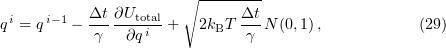
where $\Delta t$ is the time step $(0.2\ {\text{ns}}), U_{\text{total}}$ is the total energy of the system, $r$ is the monomer radius, $\eta$ is the medium viscosity coefficient, $\gamma_q=6\pi r\eta$ is the particle translational viscosity coefficient, and $\gamma_\tau =8\pi r^{\,3}\eta$ is the particle rotational viscosity coefficient [103].

The lower bound for the time step $\Delta t\gg \tau$ can be roughly estimated from a single collision time

$$\begin{equation} \tau\sim {2r_0\over \bar u}\,, \end{equation} \tag{ 30 }$$

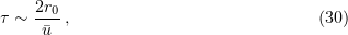
where the particle size in the medium is $2r_0\sim 5\ \mathring{\text{A}}$, and $\bar u \sim \sqrt{3k_{\text{B}}T/m}$. Hence, $\tau \sim 10^{-12}\ {\text{s}}$. The time step in the finite-difference scheme considered below is $\Delta t\sim 10^{-10}\ {\text{s}}$.

We used the Brownian dynamics technique described in preceding paragraphs to create a microtubule molecular-mechanical model [28]. Geometrically, its design replicates our earlier models with their aforementioned limitations that precluded an adequate description of microtubule dynamics [70, 71]. The elementary structural subunit of a microtubule is a tubulin monomer represented as a hard sphere with a radius of $2\ {\text{nm}}$, two left- and right-hand interaction points (lateral bonds), and two more (top and bottom) points (longitudinal bonds) in the microtubule lattice (Fig. 10).

Zoom In Zoom Out Reset image size

The proposed model has the same spatial limitation as Efremov's model [70], in which the motion of each protofilament is restricted to one plane containing the microtubule axis and the given protofilament. For this reason, each monomer is described by only three coordinates $(x_i, y_i, \tau _i)$: two Cartesian coordinates of the monomer center in the plane and the rotation angle.

The lateral interaction potential (Fig. 11) described as a function of the distance $r^{{\text{lat}}}$ between interacting sites is represented as a well with the repulsing barrier [70, 71, 95, 104]:

$$\begin{equation} \begin{aligned} V^{\text{lat}}_{k,\,n}(r_{k,\,n})&=A_{\text{lat}}\bigg({r^{\text{lat}}_{k,\,n}\over r_0}\bigg)^2\exp\bigg(-{r^{\text{lat}}_{k,\,n}\over r_0}\bigg)\cr &- b_{\text{lat}}\exp \bigg[-{(r^{\text{lat}}_{k,\,n})^2\over d r_0}\bigg]\,. \end{aligned} \end{equation} \tag{ 31 }$$

The longitudinal interaction between monomers in adjacent dimers is calculated using the formula for the lateral interaction with the parameters $A_{\text{lat}}$ and $b_{\text{lat}}$ substituted by $A_{\text{inter}}$ and $b_{\text{inter}}$. The longitudinal monomer–monomer interaction within one dimer is considered to be smooth and is calculated by the formula

$$\begin{equation} V^{{\text{intra}}}_{k,\,n}(r_i)={1\over 2}\,k r^{\,2}_{k,\,n}\,. \end{equation} \tag{ 32 }$$

The bending of protofilaments in their motion plane is described by the bending potential [see formula (10)].

Zoom In Zoom Out Reset image size

The total energy of the system as the sum of the energies of lateral, longitudinal, and bending interactions is

$$\begin{equation} U_{\text{total}}=\sum^{13}_{n=1}\sum^{K_n}_{i=1} (V^{\text{lat}}_{k,\,n}+V^{{\text{inter}}}_{k,\,n}+V^{{\text{intra}}}_{k,\,n}+g^{{\text{bending}}}_{k,\,n})\,. \end{equation} \tag{ 33 }$$

The summation is over all the 13 protofilaments (the index $n)$ and each monomer in a protofilament (the index $i$).

To find the position of a particle at given time instants, we consider the numerical solution of the Langevin equation of motion in the Brownian approximation [29]. The kinetic part of the algorithm describes tubulin attachment to the end of any protofilament and GTP hydrolysis. These events are checked every millisecond with the probability

$$\begin{equation} p=k_{\text{on}}c_{\text{tub}}\ {\text{per}}\ 1\ {\text{ms}}\,, \end{equation} \tag{ 34 }$$

where $k_{\text{on}}$ is the association constant and $c_{\text{tub}}$ is the tubulin concentration in the solution. We chose the simplest GTP hydrolysis rule: with a fixed probability regardless of the position and the environment of the attached GTP dimer. During hydrolysis, the equilibrium (zero) value of the angle $\chi^{{\text{T(D)}}}$ in formula (11) changes to 0.2.

This model is the most detailed one among the currently available microtubule dynamics models. It describes the largest set of experimental data in the framework of a single set of parameters.