

Abstract
The auditory system possesses remarkable characteristics: super sensitivity and frequency selectivity. However, these traits come at the cost of non-fidelity due to non-linear effects. The culprit behind this active behavior is likely the haircells, as suggested by some in vivo observations and theoretical studies. These haircells appear to operate as non-linear oscillators near a Hopf bifurcation. In this article, we experimentally design a single delayed Hopf resonator to examine its dynamic responses and uncover striking parallels with the human ear. After a systematic characterization of this resonator, we experimentally verify on this single resonator two non-linear phenomena that mimic hearing distortions. This provides further support for hearing models based on Hopf bifurcation.
Export citation and abstract BibTeX RIS

Published by the EPLA under the terms of the Creative Commons Attribution 4.0 International License (CC-BY). Further distribution of this work must maintain attribution to the author(s) and the published article's title, journal citation, and DOI.
Introduction
The human ear is an extremely sensitive and discriminating sensor. It is able to detect sound-wave–induced vibrations of the eardrum having a large dynamic range of 120 dB, and a wide spectral range from 20 Hz to 20 kHz [1]. To understand these impressive performances, the hearing mechanics has been first explained with the resonance theory by Helmholtz [2], but most of the knowledge is inherited from the work of Békésy [3]. His travelling wave theory states that the sound pressure applied at the entrance of the cochlea —the inner ear's part responsible for the mechano-transduction— generates an elastic vibration that propagates along the basilar membrane. This guided wave presents peaks of displacements that are located on this membrane depending on its frequencies: high frequencies are peaked at the base (the entrance) as opposed to low frequencies spreading to the apex (the other extremity of the cochlea). Nevertheless, his strategy for observing these vibrations was strongly invasive so his theory represents only the "dead" mechanics of the cochlea.
Even if Békésy did leave some of the best observations to his descendants, he did not remark some key features when studying the hearing: the oto-acoustic emissions [4] or the cochlear amplification [5] which are manifestations of the living nature of the ear. These modern explorations support the work of Gold [6] who did regard in 1948 the cochlea no longer as passive, but as an active sensor [7]. The additional source of energy in it is fundamental since it increases the dynamics of the sensor [8,9]. But, this comes with a cost: the ear is not a high-fidelity device. Indeed, two evidences of this can be sensed in the daily life. The first occurs when a second tone is played along with an original tone. The sensitivity to detect the quietness vanishes. The second tone reduces the ability to detect the original one: this is the "masking effect" [10]. Second, someone listening at once to two pure tones with nearby frequencies hears a third tone that is not in the initial acoustic signal. This distortion product is called "Tartini" or "phantom" tone [11].
Following these observations, it has been proposed that the cells operating the mechano-transduction in the inner ear, namely the haircells, are responsible for this active behaviour. And new models of the inner ear suggest that it is a collection of many critical oscillators operating near a Hopf bifurcation [12,13]. The latter denotes an oscillatory instability that involves the sudden emergence or disappearance of self-sustained oscillations as a particular parameter undergoes continuous change [14]. When this parameter reaches a specific value, namely its critical point, a change in its behavior is reached, this is the bifurcation. We can characterize this active system near the critical point as a critical oscillator, and its dynamics can be described by a dynamic equation, which we elaborate on later. This theory is supported by several experimental evidences made on isolated living haircells of bullfrogs [15–18]. In a previous study [19], the coupling between multiple resonators operating near a Hopf bifurcation was experimentally examined, successfully replicating certain characteristics of the active amplifier found in the living cochlea. In the current investigation, our focus shifts to the behavior of a single resonator, specifically emulating the behavior of a hearing hair cell that acts as a Hopf resonator, as opposed to replicating the entire cochlea. Consequently, some filtering effects resulting from the tonotopy of the cochlea are overlooked. However, this approach allows for a direct comparison to experiments conducted on isolated hair cells. The logical next step involves reintegrating the current design into a multiresonant system. Following a comprehensive and detailed description of the physical role of each parameter in the design, we delve into the consequences of its non-linear nature. This includes the identification of masking effects and the manifestation of phantom tones within this single resonator. This article presents experimental observations on such a Hopf resonator, with the theoretical framework detailed in other references [13,20,21].
The experimental resonator, featured in fig. 1, follows a basic quarter-wavelength acoustic design. It comprises a 10 cm long, 1 cm diameter Plexiglas tube with one open end and one closed end. The closure component is a 3D-printed plastic piece. This piece was meticulously designed and tested to ensure precise component fitting, and extensive trials were conducted to determine the optimal placement within the printed cap. This keen focus on 3D print design was essential to attain peak functionality for our electronics and, consequently, our feedback loop. The real goal of this design is to inject in real time a signal that is directly related to the acoustic pressure inside the tube: a feedback loop is built.

Fig. 1: A quarter-wavelength acoustic resonator converted onto a delayed resonator. A 10 cm long Plexiglas tube is terminated by a 3D printed top. A microcontroller (Adafruit Trinket M0) allows to create a feedback loop between a microphone and a speaker with their respective dedicated electronics. Measurements inside the tube are made thanks to an electret microphone connected to an extra soundboard.
Download figure:
Standard imageThe design of this resonator is a follow-up of a previous work [19] where the loop was controlled through a soundcard connected to a computer. This revealed to be very limited in the number of resonators that can be controlled in the same time. Here, the computer and its soundboard are replaced by a microcontroller (Adafruit Trinket M0) which possesses analog input and output ports. Due to digital conversion and numerical processing, a delay is introduced in the loop hence the name of delayed resonator. To probe the physics of the system we use a Presonus Audiobox soundcard that allows generating sound from outside the resonator and measuring the response with a second electret microphone placed inside. Although the diameter of this microphone is somewhat large compared to the diameter of the resonator, it did not pose any issues in measuring the response inside. In fact, we leveraged its extended wire length to facilitate its insertion and optimize measurements in close proximity to the feedback loop.
From a mathematical point of view, the pressure field p(t) near the closed end of the resonator is governed by the equation

where ω0 is the natural resonance frequency of the quarter-wavelength resonator and Q its quality factor. We will refer to these parameters as the passive parameters since they represent the response of the resonator with no feedback. S(t) is the source term corresponding to the excitation with the speaker near the open end, while  corresponds to the source term associated to the feedback. The latter can be rewritten by introducing the delay τ and the gain G(t) of the loop as

Thanks to the use of a microcontroller (or a computer as in [19]) the loop's gain G(t) or its delay τ can be modified in real time and can include complex non-linear functions. In this article, we will end on a gain that allows to mimic a system operating near a Hopf bifurcation [12]. But, before showing how we reach this ultimate goal, we describe step by step the effect of each parameter.
Resonator with a constant gain
In order to show the impact of the gain and the delay, a set of experiments is conducted where one of the values remained constant while the other varies.
Effect of the gain G0
Everything starts by setting the delay τ within the microcontroller to its smaller possible value, but one has to remember that the loop still adds an electronic delay due to the analog to digital conversion and reciprocally. Then, the gain G(t) is set to a constant value G0. The first set of experiments consists in emitting a short pulse (typically one cycle) whose central frequency corresponds to ω0. Starting from a value of G0 equal to zero, the transient field inside the tube is measured in response to this short stimulus. The measured signal corresponds to an oscillating signal with an exponential decay, as for any resonating system. The envelope of this signal is kept using the Hilbert transform and results are represented in logarithmic scale in fig. 2(a) for various values of G0. The decay rate strongly depends on the value of G0: the higher the gain, the longer the oscillations. If we keep increasing the gain, a critical value Gc is reached for which the re-injected energy matches the lost one. The attenuation time has become infinitely long.
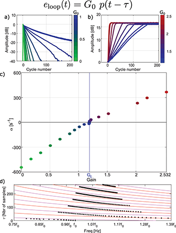
Fig. 2: Delayed resonator with static gain and delay. (a) The envelope of oscillation decaying after a pulse excitation for different values of the gain G0 below the critical gain. (b) Spontaneous growths of the envelope for different values of G0 bigger than the critical gain. (c) Exponential constant α of the respective decays and growths. (d) Influence of the delay time τ on the measured resonance frequency.
Download figure:
Standard imageAbove this critical value, the delayed resonator supports self-sustained oscillations even in the absence of stimulus: this is the well-known acoustic feedback [22,23]. No external source is needed. To probe the dynamics of the system, the experiment consists in turning off the feedback loop and measuring the transient response of the oscillator when it is turned on back. The envelope of the signals now shows an exponential increase, before reaching a saturation value of self-sustained oscillations [24]. The curves for various values of G0 above Gc are represented in fig. 2(b). The characteristic time of each experiment is extracted by a linear fit before saturation.
Combining the results of these two experiments, the graph of fig. 2(c) is built. It corresponds to the attenuation or the increase coefficient α as a function of G0. A change in sign is observed at the critical value Gc : Below this threshold α is negative and the response corresponds to damped oscillations; above this critical value α is positive and the oscillator is unstable. The relationship between α and G0 is linear.
Effect of the delay τ
To study the impact of the delay on the feedback loop, we define a delay time τs in software which corresponds to multiple values of the sampling time of the microcontroller (here the sampling frequency is chosen to be equal to 48 kHz, thus giving a resolution time of roughly 21 μs). Note that the total delay also includes the incompressible electronic ones. The measurements consist in evaluating the frequency in the limit cycle slightly above the critical gain. Repeating the experiment while changing τs one obtains the points of fig. 2(d). To understand this behaviour, we perform the Fourier transform of eq. (1):

An easy interpretation is to recall that a diverging frequency near ω0 is expected. Thus, the real part of the pole is almost ω0, and the cosine must be negligible. It occurs when  with
with  . These curves (red and pink depending on the parity of n in the figure) are an easy way to follow the experimental resonance when increasing the delay. This approach neglects the details and one can notice that the experimental resonance switches from the red curve to the pink one while increasing the delay. This is a direct consequence of the π-phase shift introduced by the passive resonance. From now, we choose τs
to be equal to 0.
. These curves (red and pink depending on the parity of n in the figure) are an easy way to follow the experimental resonance when increasing the delay. This approach neglects the details and one can notice that the experimental resonance switches from the red curve to the pink one while increasing the delay. This is a direct consequence of the π-phase shift introduced by the passive resonance. From now, we choose τs
to be equal to 0.
A non-linear resonator operating near a Hopf bifurcation
From linear to non-linear resonator
In mammalian's hearing, the outer haircells produce amplification of low sound level [25]. This effect, known as the cochlear amplifier, permits to enlarge the range of audible sound amplitudes. The transition between the low and high amplitude sounds reveals a cubic non-linearity [26]. We now aim at demonstrating that it is possible to mimic such a behaviour with our low-cost delayed resonator. We turn our resonator onto a non-linear one operating near a Hopf bifurcation. The gain is thus defined as
where the extra parameter P0 has been introduced.
The limit cases of this non-linear resonator are relatively easy to understand. At low amplitude, i.e.,  , the gain is almost G0 and the case of a static gain detailed previously is recovered. The value of G0 is chosen to be near the critical gain in order to have a high-quality factor for low amplitudes. Unlike for high amplitudes, i.e.,
  , the gain is null and a low-quality factor of a passive quarter-wavelength resonator is obtained. In between these two extreme cases, G(t) contains a square dependence on the instantaneous pressure which gives an overall cubic dependence on the pressure in the feedback.
The experiment now consists in exciting monochromatically the resonator with different amplitudes and frequencies. For each excitation, the response is measured at the same frequency. All the results are shown in fig. 3(a). Note that the definition of decibel in these experiments is arbitrary and does not correspond to true sound pressure level but rather to normalized units: a value of 0 dB is chosen for the maximal measure. As expected, an excitation with a low amplitude gives a sharp resonance (blue lines). With the increase of the excitation's amplitude, the response broadens (yellow lines) and becomes even wider (red lines) at high amplitudes.
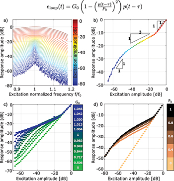
Fig. 3: An active resonator near a Hopf bifurcation. (a) The non-linear response inside the resonator is studied with respect to the excitation's normalized frequency,  (where f0 is the resonance frequency). As we manipulate both the amplitude and frequency of the incoming wave, we notice a transition from a sharp resonance at f0 for low excitation amplitudes to a progressively broader resonance as the excitation's amplitude increases. (b) The so-called sensitivity curve that mirrors data in panel (a) focuses solely on the response amplitude at f0. Notably, panel (b) reveals dual linear regimes (blue and red dots) for low and high amplitudes, with an inverse cubic response for medium amplitudes. (c) and (d): influence of G0 and P0 on the response at f0.
Download figure:
Standard imageFrom all these measurements, we build fig. 3(b), where only the response at resonance is kept. The three regimes previously discussed are easily highlighted by this curve [27]. At high amplitudes the resonator has a linear response (slope is 1): the response is proportional to the excitation. Decreasing the amplitude of excitation, an inverse-cubic power law is observed with a transition near −10 dB. This is the consequence of the cubic non-linearity in the feedback. At low amplitudes, the slope recovers a value of 1 (near −50 dB ). To get the slope of one at low amplitudes the resonator must operate in sub-critical regime where  . If not, the feedback would already be on and an activity even in the absence of excitation would happen.
Influence of the parameters
To fully complete the study, experiments are conducted where the two parameters of the feedback loop are varied separately. The role of G0 in the active mechanism is summarized in fig. 3(c). The value  corresponds to the data of fig. 3(a) and (b). Thanks to the sharpening of the resonance at low amplitude, the higher G0, the bigger the difference between the two linear parts of the response is. In other words, the value of G0 governs the amplification gain for low amplitudes compared to the high ones. When G0 is equal to 0 (green curve), a linear resonator in the entire dynamic range is recovered, and no amplification of low-amplitude sounds occurs as in a dead cochlea.
The role of P0 is presented in fig. 3(d). Again, the value of 1 corresponds to the data of fig. 3(a) and (b). P0 is the transition point between the linear regime and the inverse-cubic law. Experimentally, decreasing P0 this transition decreases from −10 dB down to −18 dB for 0.4.
Non-linear interferences in hearing
In this series of experiments, we aim to replicate non-linear effects in the behavior of the ear, particularly focusing on the masking effect. This phenomenon demonstrates that one sound's perception can be significantly influenced by the presence of another sound.
Masking effect
Our experiments involve subjecting the non-linear resonator to a two-tone excitation, where one tone operates at the resonance frequency, denoted as f1, and the second tone is labeled as f2. We measure the response at f1. In the first set of measurements (fig. 4(a)), we manipulate the amplitude of the second tone, while in the second set (fig. 4(b)), we adjust the spectral detuning. When we introduce a second tone with relatively high amplitude  and a frequency
  , the amplification for low amplitudes vanishes, resulting in a linear response at f1 (as depicted in fig. 4(a)). This high-amplitude second tone elevates the threshold of hearing for the first tone, giving it the name of "masking" tone. The higher the amplitude of this masking tone, the more pronounced its effect. When we deactivate the masking tone (as indicated in the reference curve), the amplification is naturally restored, leading to the recovery of the characteristic non-linear cubic curve shown in fig. 3(b). In the middle ground between these two limit scenarios, we observe that the impact on the low-amplitude amplifier diminishes with increasing A2 (ranging from
  to
to  ), depending on the presence and the amplitude of the second masking tone. Similarly, when the masking tone's frequency closely aligns with the resonance frequency
  , the effect becomes more pronounced compared to cases with higher detunings
  . In essence, this masking effect obscures the typical gain we observe, resulting in a linear response curve (as illustrated in fig. 4(b)).
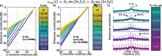
Fig. 4: Two-tone-excitation of the non-linear resonator. Panels (a) and (b) correspond to the masking effect, the response at f1 when the second tone is present with different amplitudes in (a) and with different detuning in (b). The presence of the second tone "masks" the amplification of low-amplitude sounds. Panel (c) corresponds to the generation of phantom tones: the spectral response of the non-linear resonators displays cubic distortions; and they are more pronounced at higher level.
Download figure:
Standard imagePhantom tones
The last experiment consists in reproducing the generation of phantom tones in the inner ear [11]. This is done by determining the full spectral response to a two-tone stimulus with equal amplitudes and close frequencies around the resonance frequency ( (fig. 4(c)). The response exhibits the presence of distortion products. Exciting with a weak stimulus of −42.4 dB a cubic difference products starts appearing at frequencies
  and
and  . Increasing the excitation amplitude, the cubic distortions are rapidly increasing and distortion products with an increased order are more pronounced. As opposed to the cochlea we here measure symmetric distortion peaks, because we are working with a single resonator and we do not benefit from the cochlear spatial filter.
Conclusion
To sum it up, we have succeeded in making a delayed resonator which does operate near a Hopf bifurication using only three elements: a micro-controller, a microphone and a speaker. These three agents team together building a loop where a tunable programmable non-linear gain G(t) is added. With this combination, a resonator that mimics well the response of a single bullfrog's haircell [15–18] is built. Notably, the sensitivity curve showing the low-amplitude amplifier of the cochlea is reproduced and the possibility to tune the response has been extensively studied. Not only this resonator shows the cochlear amplifier but it also exhibits two effects in hearing that come as a result of this non-linearity: the masking effect and the phantom tones.
With just one resonator working exactly as intended, the next step is naturally to couple at least two. When the coupling is sufficiently important and when the frequency is closer to the characteristic frequency all in the subthreshold Hopf regime, we expect more complex behaviours [28]. Later, by properly accomplishing a correct coupling between many resonators [29], we plan to obtain the cochlear model and get closer to the human behavioral hearing. No longer all distortions products are expected but only  when studying the phantom tones. We therefore expect to provide experimental evidence on the superiority of having a non-linear sensor for different cognitive tasks such as speech recognition or sound detection. Also, we strongly think that any cochlear implant should incorporate such non-linearities and will aim at designing them.
Acknowledgments
This work has received support under the program "Investissements d'Avenir" launched by the French Government and by the Simons Foundation/Collaboration on Symmetry-Driven Extreme Wave Phenomena.
Data availability statement: The data generated and/or analysed during the current study are not publicly available for legal/ethical reasons but are available from the corresponding author on reasonable request.