


Abstract
A model of an autonomous three-sphere microswimmer is proposed by implementing a coupling effect between the two natural lengths of an elastic microswimmer. Such a coupling mechanism is motivated by the previous models for synchronization phenomena in coupled oscillator systems. We numerically show that a microswimmer can acquire a nonzero steady state velocity and a finite phase difference between the oscillations in the natural lengths. These velocity and phase differences are almost independent of the initial phase difference. There is a finite range of the coupling parameter for which a microswimmer can have an autonomous directed motion. The stability of the phase difference is investigated both numerically and analytically in order to determine its bifurcation structure.
Export citation and abstract BibTeX RIS
Introduction
Microswimmers are small machines that swim in a fluid and they are expected to be used in microfluidics and microsystems [1]. Over the length scale of microswimmers, the fluid forces acting on them are dominated by the frictional viscous forces. By transforming chemical energy into mechanical energy, however, microswimmers change their shape and move efficiently in viscous environments. According to Purcell's scallop theorem, reciprocal body motion cannot be used for locomotion in a Newtonian fluid [2,3]. As one of the simplest models exhibiting nonreciprocal body motion, Najafi and Golestanian proposed a three-sphere swimmer (NG swimmer) [4,5], in which three in-line spheres are linked by two arms of varying length. In recent years, such a swimmer has been experimentally realized by using colloidal beads manipulated by optical tweezers [6], or ferromagnetic particles at an air-water interface [7,8].
Recently, some of the present authors have proposed a generalized three-sphere microswimmer model in which the spheres are connected by two harmonic springs, i.e., an elastic microswimmer [9]. Compared with the NG swimmer, the main difference is that the natural length of each spring (rather than the arm length) is assumed to undergo a prescribed cyclic motion. A similar model was proposed by other people [10–12]. We have analytically obtained the average swimming velocity as a function of the frequency of cyclic change in the natural length [9]. Using this model, we have also discussed the hydrodynamic interaction between two elastic swimmers [13] and a thermally driven elastic microswimmer [14–16].
In the above three-sphere microswimmer models, either the arm lengths (NG swimmer) or the natural lengths of the springs (elastic swimmer) are assumed to undergo a prescribed cyclic motion. Such active motions can lead to a net locomotion if the swimming strokes are nonreciprocal. In these models, the average swimming velocity is purely determined by the frequency and the phase difference of the prescribed motions [4,5,9,13].
On the other hand, it is beneficial for a microswimmer if the swimming velocity is autonomously determined by itself rather than being imposed externally. Moreover, a sophisticated microswimmer requires a feedback control system in order to regulate the switching between the static and swimming states by tuning the system parameters. For a macroscopic quadruped robot (not a swimmer), it was demonstrated that the communication between legs during movements is essential for interlimb coordination in quadruped walking [17,18]. A similar mechanism is also useful for the locomotion of a microswimmer.
In this letter, extending the mechanism of an elastic swimmer [9], we propose a new type of three-sphere swimmer which can autonomously determine its velocity. In order to implement such a control mechanism, we introduce a coupling between the two natural lengths of an elastic microswimmer by using the interaction adopted in the Kuramoto model for coupled oscillators [19–22]. Importantly, the proposed microswimmer acquires a steady state velocity and a finite phase difference in the long-time limit without any external control. The steady state velocity can be mainly tuned by changing the coupling parameter in the model. Moreover, we investigate the condition that a microswimmer can attain an autonomous locomotion, and further perform a linear stability analysis of the steady state.
Synchronization phenomena are widely observed in active biological systems such as flagella and cilia [23,24]. In particular, synchronization of a pair of flagella in Chlamydomonas was observed experimentally [25,26]. For a three-sphere model of Chlamydomonas in which the spheres representing the flagella move on circular trajectories relative to the body sphere [27,28], the two flagella can synchronize due to the local hydrodynamic friction forces [27]. On the other hand, hydrodynamic interaction between the flagella is indispensable for the net swimming.
Model of an autonomous microswimmer
As schematically shown in fig. 1, the present model consists of three hard spheres of the same radius a connected by two harmonic springs characterized by the spring constant K. The total elastic energy is given by

where  are the positions of the three spheres in a one-dimensional coordinate system and we assume x1 < x2 < x3 without loss of generality. In the above,
  and
and  are the natural lengths of the springs and their dynamics will be explained later (see eqs. (7) and (8)). Each sphere exerts a force on the viscous fluid of shear viscosity η and experiences an opposite force from it.

Fig. 1: An autonomous elastic microswimmer in a viscous fluid characterized by the shear viscosity η. Three identical spheres of radius a are connected by two harmonic springs characterized by the spring constant K. The time-dependent positions of the spheres are denoted by x1, x2, and x3 which evolve in time according to eq. (2). The time-dependent natural lengths of the springs are denoted by  and
and  whose dynamics is described by eqs. (5) and (6), respectively, whereas the corresponding phases
  and
and  obey eqs. (7) and (8), respectively.
Download figure:
Standard imageDenoting the velocity of each sphere by  and the force acting on each sphere by fi
, we can write the equations of motion of each sphere as [9,13]
and the force acting on each sphere by fi
, we can write the equations of motion of each sphere as [9,13]

where the three forces fi are given by

Here the details of the hydrodynamic interactions are taken into account through the mobility coefficients Mij
. Within Oseen's approximation, which is justified when the spheres are considerably far from each other  , the expressions for the mobility coefficients Mij
can be written as
, the expressions for the mobility coefficients Mij
can be written as

The force-free condition,  , is automatically satisfied in the present model [9,13]. We define the center-of-mass position of a microswimmer by
  and the swimming velocity of the whole object by
  .
.
Next, we consider that the two natural lengths of the springs undergo the following cyclic changes in time [9,13]:


where ℓ is the constant natural length, d is the oscillation amplitude,  and
and  are the time-dependent phases. The most important aspect of our model is that
  and
and  are affected by the relative positions and the velocities of the three spheres. We employ the following time evolution equations for
  and
and  which are often used to describe synchronization phenomena [19]:


where Ω is the constant frequency, α is the coupling parameter describing the strength of synchronization, and  and
and  are the mechanical phases as explained below.
To define the above mechanical phases for a three-sphere model, it is convenient to introduce the following spring lengths  and
and  with respect to ℓ:


Obviously, these quantities are related to the sphere velocities as  and
and  . Then the time-dependent mechanical phases
  and
and  are introduced by the relative positions and the velocities of the spheres as


where ![$D_{\rm A(B)}=[u_{\rm A(B)}^{2}+(\dot{u}_{\rm A(B)}/\Omega)^2]^{1/2}$](https://content.cld.iop.org/journals/0295-5075/133/3/34001/revision2/epl20432ieqn38.gif) . Physically, the mechanical phase
. Physically, the mechanical phase  specifies the position in the phase space of a micromachine spanned by
  and
and  as shown in fig. 2.

Fig. 2: Dynamics of  describing the phase of the natural length (see eq. (5)) and
  describing the mechanical phase (see eq. (11)). When
  at t, as shown in the left figure, and when
  in eq. (7), the velocity
  becomes larger at a later time
  , as shown in the right figure. As a result, the difference between
  and
and  also increases at
  . A similar dynamics occurs also for
  and
and  .
.
Download figure:
Standard imageThe above equations complete our model for an autonomous three-sphere microswimmer. In this letter, we shall consider the case of  . Then the physical meaning of eqs. (7) and (8) is that the phase
  for the natural length and the mechanical phase
  tend to be different due to the coupling term, as schematically shown in fig. 2. Since the middle sphere is connected to the other two spheres, our model contains a feedback mechanism that regulates the dynamics of the two natural lengths
  and
and  . Such a coupling effect in the spring motions gives rise to a non-reciprocal body motion and results in an autonomous locomotion of the microswimmer. Although α in eqs. (7) and (8) can be different, we shall first stick to the symmetric case for the sake of simplicity. In general, the other quantities such as K, ℓ, and Ω can also be asymmetric.
Let us define the time-dependent phase difference between the oscillations in the natural lengths by  . When
  , the present model reduces to that of the original elastic microswimmer [9,13]. In this limit, we have
  and
and  , where
  is the initial phase difference. According to Purcell's scallop theorem [2,3], an elastic microswimmer can exhibit a directed motion when
  , i.e., a nonreciprocal motion. Hence the initial phase difference
  and the frequency Ω fully determines the average velocity of locomotion when
  [9,13].
When the coupling effect is present, however, we show that a stable phase difference δ controls the dynamics of a micromachine irrespective of its initial value  . Moreover, the transition to a nonreciprocal motion as well as the average velocity can be precisely tuned by the coupling parameter α and the velocity is not solely fixed by the externally given frequency Ω as in the previous models [4,5,9,13].
For numerical simulations, it is convenient to introduce a characteristic time scale defined by

which represents the spring relaxation time. Then we use ℓ to scale all the relevant lengths (such as xi
, a, and d) and employ τ to scale the quantities related to time (such as Ω and α). All the dimensionless variables and parameters are written with a hat such as  ,
,  , and
, and  .
.
Simulation results
First we have performed computer simulations by numerically solving eq. (2) together with eqs. (5)–(12) with the use of Euler's method. The parameters to characterize the swimmer size are chosen as  and
and  , satisfying the conditions
  . Concerning the initial conditions, we put the three spheres at
  ,
,  , and
, and  , whereas the initial phase difference,
  , is varied within the range
  . In the present work, we focus on the low-frequency regime,
  . The following simulation results do not depend on the initial positions of the three spheres.
In fig. 3, we plot the dimensionless center-of-mass position  as a function of time
  for different values of the coupling parameter
  when (a)
  and (b)
  , whereas the frequency is fixed to
  . Although
  also oscillates in time at much smaller time scales, as shown later in fig. 4(a), one can extract an average steady state velocity
  in the long-time limit by fitting with a straight line. We estimate such an average velocity
  for each curve in fig. 3, and regard it as an autonomously determined steady state velocity. For
  (black),
  vanishes both in figs. 3(a) and (b). For
  (red), on the other hand,
  is finite in fig. 3(a) but vanishes in (b). In this case, the steady state velocity depends on
  . For
. For  (green),
  is the same between figs. 3(a) and (b), showing that
  does not depend on the initial phase difference
  although the sign of
  can change as we show later in fig. 5(a).

Fig. 3: The plots of dimensionless center-of-mass position  of an autonomous three-sphere microswimmer as a function of dimensionless time
  for
for  when the initial phase differences are (a)
  and (b)
  . In both plots, the dimensionless coupling parameter is chosen as
  (black), 0.5 (red), and 2 (green).
Download figure:
Standard image
Fig. 4: The plots of (a) dimensionless center-of-mass position difference  and (b) the phase difference
  between the oscillations in the natural lengths as a function of dimensionless time difference
  measured from
  when
when  and
and  . In both plots, the dimensionless coupling parameter is chosen as
  (black), 0.5 (red), and 2 (green). The average steady state velocity
  is obtained by fitting with a straight line, whereas the steady state phase difference
  is obtained by averaging over a cycle in the oscillations of δ.
Download figure:
Standard image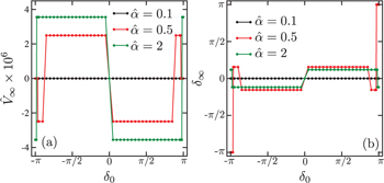
Fig. 5: The plots of (a) dimensionless stationary velocity  and (b) stationary phase difference
  as a function of the initial phase difference
  when
when  . In both plots, the dimensionless coupling parameter is chosen as
  (black), 0.5 (red), and 2 (green). Notice that, for each color, there are multiple data points close to
  .
.
Download figure:
Standard imageIn figs. 4(a) and (b), the behaviors of the center-of-mass position difference  and the phase difference δ at much smaller time scales are plotted, respectively, as a function of the time difference
  measured after
  . Since the other parameters are
  and
and  , fig. 4(a) is the magnification of fig. 3(a) in the long-time limit after the steady state has been reached. It is important to note that both
  and δ exhibit oscillatory behaviors whose period becomes smaller as α is increased. Such a change in the period is consistent with a perturbation expansion of eqs. (7) and (8) in terms of α, as we shall explain later. In fig. 4(b), the phase difference δ oscillates around a constant value that can be regarded as the steady state phase difference
  . Here, we define
  as the average over a cycle in the oscillations of δ. Since there is always a well-defined steady state for a given set of parameters, further simulations have been performed for different values of
  to investigate the behaviors of
  and
and  systematically.
Fixing the frequency to  , we plot in figs. 5(a) and (b) the steady state velocity
  and the phase difference
  , respectively, as a function of the initial phase difference
  for the range
  . Different colors indicate different
  values as we have used in fig. 3. In fig. 5(a), we see that
  either vanishes or takes a nonzero constant value within a certain range of
  . This means that, under certain conditions, the proposed microswimmer can autonomously determine its steady state velocity as well as the phase difference. We also see that
  changes its sign at
  although the absolute value is the same. The sign of
  and
and  also changes for
  (red) and 2 (green) when
  becomes close to
  .
.
For  (red) in fig. 5(a), the velocity
  tends to vanish when the initial phase difference
  is close to
  . In this situation, we see in fig. 5(b) that the steady state phase difference approaches
  , i.e., a reciprocal motion. When
  is finite in fig. 5(a) for
  (red) and 2 (green), on the other hand, the corresponding phase difference is
  , i.e., a nonreciprocal motion. These results are in accordance with Purcell's scallop theorem [2,3]. A more detailed discussion concerning the stability of the phase difference will be given later in fig. 7. When
  , there are two stable fixed points; one with finite
  and the other with vanishing
  .
.
In figs. 6(a) and (b), we plot  and
and  , respectively, as a function of
  for different frequencies
  , 0.1, and 0.2. To make these plots, we have used
  . When
  (orange), for example, there is a finite critical value of
  above which
  and
and  become nonzero. For
  , on the other hand, both
  and
and  vanish. The existence of such a finite critical value
  is a nontrivial outcome of the present model. When
  is very large, such as
  for
for  , both
  and
and  vanish again. Hence autonomous locomotion can be achieved for a finite range of the coupling parameter
  . Such a behavior is common for other frequencies
  .
.
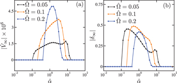
Fig. 6: The plots of (a) dimensionless stationary velocity  and (b) stationary phase difference
  as a function of the dimensionless coupling parameter
  . In both plots, the dimensionless frequency is chosen as
  (black), 0.1 (orange), and 0.2 (blue), while
  is fixed. There is a lower critical value
  above which both
  and
and  become nonzero.
  and
and  take maximum values at
  , and they vanish for large α.
Download figure:
Standard imageMoreover, it is interesting to note that  takes maximum values such as at
  when
when  . Hence the present autonomous microswimmer can maximize its velocity by tuning the coupling parameter α. Notice that both
  and
and  depend on the frequency
  , and they are not universal quantities. However, it is worth mentioning that we find the relation
  for all
  chosen in our simulations.
From these simulation results, one can discuss the stability of the relative phase difference δ. Comparing its initial value  and the steady state value
  , we can identify the stable fixed points. Such a stability diagram for
  is presented in fig. 7 in the plane of δ and
  , describing the bifurcation structure of the present model. The orange circles indicate the stable fixed points where
  holds. In fig. 7 we have also plotted the numerically determined separatrices by the dashed lines. These points are obtained by comparing the initial phase difference
  and the stationary phase difference
  . Hence they are not mathematically obtained rigorous unstable points.
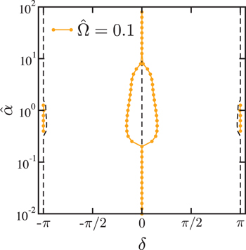
Fig. 7: The numerically obtained stability diagram in the plane of the phase difference δ and the dimensionless coupling parameter  when
when  . The orange circles indicate stable fixed points where
  holds. For
  , the stable point
  bifurcates into two stable fixed points. These nonzero fixed points correspond to nonreciprocal motions
  , leading to a nonzero velocity
  . There are other stable fixed points at
  when
when  . For larger
  ,
,  becomes stable again for
  . The dashed lines indicate the numerically determined separatrices which are obtained by comparing the initial phase difference
  and the stationary phase difference
  .
.
Download figure:
Standard imageFor  , the stable fixed points exist only at
  . As
. As  is increased, the stable point at
  bifurcates into two stable fixed points for
  , whereas
  becomes unstable. The stable fixed points at nonzero δ correspond to nonreciprocal motions, leading to finite
  and
and  . When
  satisfies
  , the two stable fixed points at
  appear. These new fixed points result in a reciprocal motion, prohibiting the locomotion of a microswimmer. For larger coupling parameter
  ,
,  becomes stable again. Although such a stability diagram depends on
  , the general structure of the bifurcation diagram remains the same.
Linear stability analysis in the weak coupling limit
Although the equations of motion of our model are highly nonlinear, we can analytically investigate the linear stability of the phase difference δ when  is small enough. In other words, we consider the case
  in fig. 7, for which
  is the only stable point and a microswimmer exhibits a reciprocal motion. Here, we shall express
  in terms of δ and perform a stability analysis. Starting from eq. (2), we first neglect hydrodynamic interactions by considering the case
  . Then the equations of motion for
  and
and  (see eqs. (9) and (10)) are approximated as


where τ is the spring relaxation time introduced in eq. (13).
When the coupling parameter α is small enough in eqs. (7) and (8), one can assume that δ is almost constant and the phases of the two natural lengths can be approximated as  and
and  . According to ref. [9], the coupled linear equations in eqs. (14) and (15) can be solved in the frequency domain. By performing the inverse Fourier transform, we have
where  as before and δ here is a constant.
The above results can be inserted into eqs. (11) and (12) to obtain  and
and  , respectively. Considering the low-frequency limit,
  , we expand
  and
and  up to the second order in
  :
:


Then we substitute these expressions into eqs. (7) and (8) to obtain


where we have used the approximations  and
and  . The stability of δ can be discussed in terms of
  that is given by

In fig. 8, we plot  as a function of δ for
  , 0.1, and 0.2. We first note that eq. (22) is an odd function of δ. Since
  for
for  and
and  for
for  , we find that
  is a stable fixed point. This result is in accordance with the stability diagram in fig. 7 when
  . The slope at
  becomes steeper as
  is increased. We also see that
  are the unstable fixed points.

Fig. 8: The plot of  (see eq. (22)) as a function of δ for different dimensionless frequencies
  (black), 0.1 (orange), and 0.2 (blue). Here
  corresponds to the stable fixed point, while
  are unstable ones. This result is in agreement with the stability diagram in fig. 7 when
  .
.
Download figure:
Standard imageUp to the first order in  , we see in eqs. (18) and (19) that the mechanical phases
  and
and  are delayed with respect to those of the natural length
  and
and  , respectively. Thus, the time evolutions of
  and
and  are accelerated by the second terms in eqs. (20) and (21) that are controlled by α. Hence, as α is increased, the oscillation frequencies of
  and δ become larger than the original spring frequency Ω. Such a change of the oscillation frequency was shown in fig. 4(b).
Within the present approximation, however, we cannot analytically predict the critical value  nor the stable fixed points at nonzero δ for
  . The difficulty arises because eqs. (16) and (17) are correct only for small α. Moreover, hydrodynamic interactions, which are neglected in the above analysis, need to be further taken into account to fully discuss the bifurcation structure of the model.
It is worth mentioning, however, that the stability of the phase difference δ can be determined even in the absence of hydrodynamic interactions as we have discussed in this section. For a three-sphere model of Chlamydomonas, it was shown that hydrodynamic interactions contribute little to synchronization [27]. In the present model as well as in the previous models [4,5,9,13], hydrodynamic interactions play an essential role for the locomotion of a three-sphere microswimmer.
Summary and discussion
In this letter, we have proposed a model of an autonomous three-sphere microswimmer by considering a coupling effect between the two natural lengths of an elastic microswimmer [9]. Our model is motivated by the previous models for synchronization phenomena in coupled oscillator systems [19–22]. Performing numerical simulations, we have shown that a microswimmer can acquire a nonzero steady state velocity  that is almost independent of the initial phase difference
  (see fig. 5(a)). The corresponding phase difference
  between the oscillations in the natural lengths becomes also finite (see fig. 5(b)), which is consistent with Purcell's scallop theorem for microswimmers in a viscous fluid [2,3].
We have explored in detail the dependencies of  and
and  on the coupling parameter α and the frequency Ω. We find that both
  and
and  take nonzero values for
  , and they also show maximum values at
  (fig. 6). There is a finite range of α for which a microswimmer can have an autonomous directed motion. We have also analyzed the stability of the phase difference δ by constructing a stability diagram (fig. 7). This result has been analytically confirmed in the limit of small α (fig. 8).
In the present work, we have discussed the case when the frequency Ω is small enough, i.e.,  . When Ω is made larger, the difference between
  (phases of the natural lengths) and
  (mechanical phases) becomes also larger. In the original elastic microswimmer without any coupling effect, it was shown that the average velocity decreases with increasing frequency in the high-frequency limit due to the intrinsic spring relaxation dynamics [9,13]. Such a reduction of the velocity in the high-frequency regime also occurs for a three-sphere microswimmer moving in a viscoelastic medium [29–31]. Our future numerical and analytical studies include not only the high-frequency behavior of the model but also the case of
  .
.
Acknowledgments
We thank T. Kato for useful discussions. YK acknowledges support by a Grant-in-Aid for JSPS Fellows (Grant No. JP19J00365) from the Japan Society for the Promotion of Science (JSPS). YH acknowledges support by a Grant-in-Aid for JSPS Fellows (Grant No. 19J20271) from the JSPS. KY acknowledges support by a Grant-in-Aid for JSPS Fellows (Grant No. 18J21231) from the JSPS. YK, HK and SK acknowledge support by a Grant-in-Aid for Scientific Research (C) (Grant No. 19K03765) from the JSPS. SK further acknowledges support by a Grant-in-Aid for Scientific Research (C) (Grant No. 18K03567) from the JSPS, and support by a Grant-in-Aid for Scientific Research on Innovative Areas "Information Physics of Living Matters" (Grant No. 20H05538) from the Ministry of Education, Culture, Sports, Science and Technology of Japan.