

Abstract
This letter presents a magnetic target inversion method that does not vary with changes in the coordinate system and is based on the cross-product of the intermediate eigenvectors of any two points in the dipole field which is in the same/opposite direction as the magnetic moment vector. We used tensor geometric invariants to interpret this new physical property and obtain the unit magnetic moment vector. Using this, the unit vector of the measurement point-source displacement vector was derived. The distance between the measurement point and the source was obtained via the Frobenius norm of the gradient tensor matrix. Simulations verified that the proposed method is unaffected by attitudes and yields unique inversion results, and the results revealed that the inversion accuracy of the proposed method is high. The simulation results also show that conditional cosine and measurement noise have considerable influence on the inversion accuracy in the proposed method.
Export citation and abstract BibTeX RIS

Published by the EPLA under the terms of the Creative Commons Attribution 3.0 License (CC-BY). Further distribution of this work must maintain attribution to the author(s) and the published article's title, journal citation, and DOI.
Introduction
In a geomagnetic field, objects containing ferromagnetic materials are magnetized and generate magnetic fields. Such magnetic fields superimposed on the geomagnetic field generate geomagnetic distorsions, called magnetic anomalies [1,2]. Magnetic anomaly detection technology, which locates and identifies magnetic targets by observing and analysing such anomalies [3], has been widely used in unexploded ordnance detection [4–6], underwater magnetic tracking [7,8], intruder detection [9], biomedical applications [10], geophysics exploration [11], indoor localization [12], and other fields owing to its advantages of good concealment and strong anti-interference ability. Magnetic anomaly detection technology has undergone several stages, from total magnetic field measurement, to magnetic field component and gradient measurement, to magnetic gradient tensor measurement. Magnetic gradient tensor measurement possesses a significant advantage over other traditional magnetic field measurement methods. It not only effectively suppresses the interference of the geomagnetic field, but also contains more magnetic source information [13,14]. Therefore, the magnetic gradient tensor has been widely used.
There are two main methods for inverting dipoles using the magnetic gradient tensor. The first category was proposed by Nara et al. [15]. They proposed a closed-form localization formula that combines the magnetic gradient tensor and the magnetic field vector. This method measures the magnetic field generated by the magnetic target, and the magnetic field measured by the sensor cannot be easily separated from the geomagnetic field, inducing a large error in the localization results. Based on the Nara method, Li Guang et al., Yu Zhentao et al., and Yin et al. proposed magnetic dipole localization methods based on the high-order difference in magnetic induction intensity [4,16]. These methods overcome the interference of the geomagnetic field well, but the high-order difference is greatly affected by noise, leading to high instrumental accuracy requirements. The numerical estimation method provides another approach for magnetic target inversion, mainly including linear statistical analysis and nonlinear numerical calculation. Barrell et al. [17] and Vaizer et al. [18] estimated the magnetic target parameters using linear statistical analysis. Nonlinear numerical methods, such as recursive Bayesian estimation [1], Monte Carlo [19], and downhill simplex inversion algorithms [20], have also been utilized to invert the magnetic targets using magnetic gradient tensor data. Although the results of numerical estimation methods are more robust to noise, these methods are too complex to be applied for real-time tracking.
The inversion of magnetic targets using magnetic gradient tensor achieves good results, but the magnetic gradient tensor measurement is easily affected by the attitudes, which limits its application. Tensor invariants do not vary with the change of the coordinate system, which can help overcome the influence of carrier attitudes, and they have become a research hotspot. Dipole inversion methods based on tensor invariants are mainly realized using the magnetic gradient tensor matrix Frobenius norm and normalised source strength. Wiegert and Oeschger [21] proposed the scalar triangulation and ranging (STAR) method, which was derived from the Frobenius norm of the magnetic gradient tensor matrix. This method not only overcomes the disturbance of the geomagnetic field effectively but can also be applied to mobile-carrier platforms. However, the solution of this method contains a non-circular coefficient [22], which induces large errors in the localization algorithm. There are many modification methods based on STAR, and their inversion results have been greatly improved [2,23]. Clark [24] proposed the dipole localization method via normalised source strength and applied this method to many simple models. This method allows the estimation of source location directly, without triangulation based on estimated directions to the source. The dipole inversion methods based on tensor invariants overcome the influence of attitude change and expand the application range of magnetic anomaly detection technology. The tensor geometric invariants are similar to the tensor invariants and also do not vary with the coordinate system. The difference is that tensor invariants are scalars, while tensor geometric invariants are in the form of geometric relationships. Presently, the applications of tensor geometric invariants are still few.
A common problem with the aforementioned methods is that the calculation of the target magnetic moment is heavily dependent on the localization result. The method proposed herein first identifies the target, avoiding such a problem. In this study, the cross-product of the intermediate eigenvectors of two measurement points is the direction (or reverse) of the magnetic moment derived using the spatial geometric relationships of the intermediate eigenvector, measurement point-source displacement vector, and magnetic moment vector. Based on this, the unit vector of measurement point-source displacement vector was obtained. Then, the analytical expression of the distance between the measurement point and the source was derived using the Frobenius norm. Thus far, the recognition and localization of the dipole were achieved. The proposed method does not vary with the coordinate system, and the recognition of the target does not depend on the localization result. Multiple solutions will occur during the solution process, but the ghost solutions can be quickly eliminated by using the tensor geometric invariants of the second measurement point. Finally, simulations were conducted to verify the feasibility of the proposed method. The simulation results revealed that the proposed method has high accuracy, good real-time performance, and is unaffected by attitudes. The main innovations of this study are as follows: 1) The concept of tensor geometric invariants is proposed, and a new magnetic dipole localization and recognition method is derived by using it. 2) The cross-product of the intermediate eigenvectors between two measurement points in the same (or opposite) direction as the magnetic moment vector is found. 3) A new measurement point-source distance calculation method is derived. 4) It is determined that the identification of magnetic targets by the proposed method does not depend on the localization results.
Magnetic gradient tensor theory and tensor geometric invariants
Magnetic gradient tensor of magnetic dipole
A magnetic field is a vector field, and the rates of change of the three components of this field in three directions are the magnetic gradient tensor. The magnetic gradient tensor can be expressed as the matrix multiplication of two three-element vectors. According to Maxwell's equation, in an observation area without space current density, the divergence and curl of the magnetic induction intensity are both zero [4]. Therefore, the magnetic gradient tensor matrix can be expressed as follows:
Among these, Bx, By, and Bz are the components of the magnetic field vector B in three directions orthogonal to each other, and Bij, where  , denotes the tensor components.
  is a real symmetric matrix, so it can be decomposed as follows:

where  ,
,  , and
, and  are eigenvalues and
  ,
,  , and
, and  are the corresponding mutually orthogonal eigenvectors. Eigenvalues are tensor invariants that do not vary with changes in the coordinate system, and the combinations of eigenvalues are still tensor invariants.
When the detection distance exceeds 2.5 times the length of the magnetic target, the magnetic target can be considered as a magnetic dipole [4]. For the static magnetic field, if the dipole moment is  and the displacement vector from the dipole to the measurement point is
  , then the measured magnetic field vector is

where  is the permeability,
  is the unit vector of
  ,
,  ,
,  is the unit vector of
  , and
, and  . The magnetic gradient tensor components of the dipole can be obtained using the following formula:

where  denote the component of the Cartesian coordinate axis, and
  is the Kronecker delta.
Magnetic dipole tensor geometric invariants
The geometric relationships between the eigenvectors of the gradient tensor matrix, magnetic moment vector, and measurement point-source displacement vector do not vary with changes of the coordinate system, so they can be called tensor geometric invariants. The tensor geometric invariants remain unchanged in all coordinate systems, and the Cartesian coordinate system shown in fig. 1 is selected for convenience of calculation. The dipole is located at the origin, the magnetic moment  , and the measurement point is located at
  . In this case, the magnetic gradient tensor matrix of dipole can be simplified to

where

The three eigenvalues of the dipole gradient tensor matrix, in non-increasing order, are
the corresponding eigenvectors are

It can be found from eqs. (8) that the intermediate eigenvector  is perpendicular to the magnetic moment vector
  as well as the displacement vector
  . This can be found using eqs. (7),

it is obvious that μ is non-negative, so

From eqs. (10) and (7), we conclude that

That is, the angle between the magnetic moment vector and the displacement vector is a scalar, which does not vary with changes in the coordinate system. Using CT to denote the Frobenius norm of the matrix, the Frobenius norm of the dipole gradient tensor matrix can be expressed as


Fig. 1: A schematic of the canonical coordinate system of a dipole and measurement point.
Download figure:
Standard imageThe geometric relationships among intermediate eigenvector  , magnetic moment vector
  , and displacement vector
  and the angle relationship between magnetic moment vector
  and distance vector
  do not change with the coordinate system, so they are tensor geometric invariants. The intermediate eigenvector
  is perpendicular to the magnetic moment vector
  and the displacement vector
  , implying that
  is perpendicular to the plane comprising the magnetic moment vector
  and the displacement vector
  . This spatial relationship is also a tensor geometric invariant. Herein, these tensor geometric invariants are used to invert the dipole.
Magnetic dipole localization and identification principle based on tensor geometric invariants
Calculation of unit magnetic moment vector of magnetic dipole
The planes comprising different measurement point-source displacement vectors and magnetic moment vector all contain the magnetic moment vector, so these planes intersect at the magnetic moment vector, as shown in fig. 2. In a dipole magnetic field, the intermediate eigenvector of the measurement point is perpendicular to the plane comprising the displacement vector and the magnetic moment vector. Using this tensor geometric invariant and the coordinates of the measurement point, the plane equation containing the displacement vector and the magnetic moment vector can be obtained. The direction of the magnetic moment vector can be obtained by determining the intersection line of these planes.
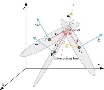
Fig. 2: Schematic of the intersection line of multiple planes composed of different measurement point-source displacement vectors and magnetic moment vector.
Download figure:
Standard imageAssuming that the position of the n-th measurement point is  and the intermediate eigenvector of the n-th measurement point is
  , the equation of the plane containing the n-th measurement point-source displacement vector and the magnetic moment vector is as follows:

These planes intersect, and the line of intersection is collinear with the magnetic moment vector. Two planes can be arbitrarily selected to find the intersection line, and the intersection direction is the same or opposite to the magnetic moment vector. The direction of the intersection line can be obtained by the cross-product of the two plane normal vectors. The intermediate eigenvector of the measurement point is the plane normal vector, so the unit vector of the magnetic moment is

where  and
and  denote intermediate eigenvectors of the i-th and j-th measurement points. In order to ensure that the two planes intersect and the intersection line is unique, the two selected planes cannot coincide. The spatial relationship between two planes can be characterized by the included angle between them, and the absolute value of the included angle cosine is called the conditional cosine. The conditional cosine can be obtained by the dot product of the unit normal vectors of two planes. After the unit vector of the magnetic moment is known, if the magnitude of the magnetic moment is obtained again, the magnetic moment vector can be obtained. There are many methods to solve the amplitude of the magnetic moment vector. However, these methods are not the focus here. The identification method proposed in this letter refers to the direction of solving the magnetic moment vector.
Calculation of displacement vector from measurement point to source
Using the geometric relationships between the measurement point-source displacement vector and magnetic moment vector, and the measurement point - source displacement vector and intermediate eigenvector, the following equations for unit displacement vector can be obtained:

Solving eq. (15) can yield the unit measurement point - source displacement vector, which only requires data of one measurement point.
The displacement vectors from measurement point  and
and  to magnetic source are
  and
and  , respectively, and the displacement vector from
  to
to  is
is  , as shown in fig. 2. After obtaining the unit magnetic moment vector of the magnetic source using the intermediate eigenvectors of
  and
and  , the unit vector
  of
of  can be obtained using the data of the
  from eq. (15). To locate the magnetic source, it is necessary to obtain the distance r1. According to the positional relationship of the measurement points, the following equation can be obtained:

From eq. (16), the distance r2 can be obtained as

The Frobenius norms of the measurement points  and
and  are CT1 and CT2, respectively. The ratio of CT1 and CT2 can be obtained using eqs. (6) and (12) as follows:

where  and
and  are the included angles between displacement vector
  and magnetic moment vector
  , and displacement vector
  and magnetic moment vector
  , respectively. Equation (18) can be transformed into

where CT1, CT2,  , and
, and  can be calculated from the gradient tensors of
  and
and  , so the right side of eq. (19) is known. For convenience of calculation, let
  , then eq. (19) becomes

By substituting eq. (17) into eq. (20), following equation is obtained:

In eq. (21), only r1 is an unknown quantity, and the distance between the measurement point  and the source can be obtained by solving it. Multiplying r1 with
  , we can obtain the displacement vector
  , thereby realizing the localization of the magnetic target.
Implementation issues
The inversion process of the proposed method will produce multiple solutions, but the ghost solutions can be quickly eliminated using tensor geometric invariants. In the foregoing process of solving the unit measurement point - source displacement vector, only the spatial geometric relationship of the  is utilized. Using the measurement information of the
  to verify whether the solved displacement vector
  is true, the ghost solutions can be eliminated. The steps to eliminate the ghost solutions are as follows:
- 1)
- 2)Calculate the eigenvalues and eigenvectors of the P2 point gradient tensor matrix, and then calculate
 using eq. (11).
 - 3)The intermediate vector of the point is perpendicular to , that is, is required. Use this constraint to eliminate ghost solutions.
- 4)The angle between the displacement vector and the magnetic moment vector is , that is, is required. Use this constraint to further eliminate ghost solutions.


Through the above steps, the location of the magnetic source can be determined uniquely, and the ghost solution of the unit magnetic moment vector can be eliminated.
Simulations
In order to estimate the theoretical accuracy of the proposed method, multiple sets of simulations were carried out. In practical applications, magnetic gradient tensors need to be obtained by differential approximation calculations [4]. In this study, a cross-structured sensor array was used to measure the magnetic gradient tensor. The target magnetic moment amplitude was  , the azimuth of the magnetic moment direction was
  , and the inclination was
  . In the following theoretical examples, it was assumed that the target magnetic moment was not affected by external magnetic fields. The Earth's magnetic field was assumed to be
  with the inclination and declination angles being 50 deg and
  , respectively. The dipole moved along a circular trajectory with a radius of 5 m on the plane of
  . A vector magnetometer with an accuracy of 0.1 nT was selected for the sensor array, and the baseline distance d between coaxial sensors was 0.2 m. The positions of the two measurement points were
  , and
, and  . Three simulations were performed, and the attitude of each simulated sensor array was different.
The localization results of the three simulations are shown in figs. 3, 4, and 5. Among them, fig. 3 presents the estimation results of the three simulated XY planes, fig. 4 presents the absolute error between the estimated position and the true value of the three simulations, and fig. 5 depicts the angular error between the unit magnetic moment vector calculated based on the three simulations and the true direction. It can be seen that the localization results of the three attitudes are approximately the same, which proves that the proposed method is not affected by the attitude. The average relative errors of the three simulated localization results were 0.2%, 0.25%, and 0.19%, respectively. The average angular errors of the three simulated recognition results were 0.09°, 0.1°, and 0.09°, respectively. It can be seen that the localization and identification accuracy of the proposed method are high. The unsolvable point occurs because the two measurement planes coincide, and the intersection line of the two planes cannot be obtained at this time.

Fig. 3: Estimation results of three simulated XY planes.
Download figure:
Standard image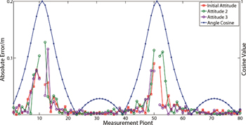
Fig. 4: Absolute errors between estimated positions of three simulations and the true value; conditional cosine corresponding to each inversion position is also presented in the figure.
Download figure:
Standard image
Fig. 5: Angular errors between unit magnetic moment vector calculated by three simulations and the real direction; the conditional cosine corresponding to each inversion position is also presented in the figure.
Download figure:
Standard imageAlthough the accuracy of the proposed method is high in theory, errors still occur in the inversion results. The errors in the simulated results consist of two main parts. The first part is the self-error caused by the defect in the proposed method, and the second part is the introduction error in the measurement process. The introduction error is mainly due to the differential approximation of the gradient tensor measurement. The self-error is caused by the relative position of the two measurement planes. If the two measurement planes are near to coincidence, the solution of the intersection line between the two planes becomes difficult, resulting in a larger inversion error. The relative position of the two measurement planes can be reflected by the conditional cosine, and the conditional cosine corresponding to each inversion position is presented in figs. 4 and 5. It can be seen that the localization effect and the identification effect are closely related to the conditional cosine. The closer the value of the conditional cosine to 1, the worse the localization and identification effect. When the conditional cosine is equal to 1, there is no solution. If the conditional cosine is less than 0.9, the relative positions of the two measurement planes will no longer affect the inversion effect of the proposed method.
Noise is inevitably introduced in a real measurement process, thereby increasing the uncertainty in dipole inversion. Therefore, resistance to noise is an important criterion for characterizing the usefulness of the inversion method. Figure 6 shows the estimated results of XY plane using the proposed method, in which a noise of 2 nT RMS was added to sensor measurements while the other conditions remained unchanged. At this time, the localization accuracy of the proposed method was significantly reduced. The specific effects of measurement noise on the proposed method are analysed as follows.
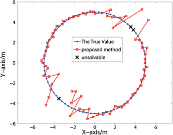
Fig. 6: XY plane estimation results when SNR = 30.
Download figure:
Standard imageThe dipole still moved on the plane of  ; however, the moving region was limited to
  and
and  to ensure that the condition cosine was sufficiently small. The moving steps of dipole in X and Y directions were 0.04 m. Gaussian noise was added to the sensor data to produce specific SNR values. With other conditions remaining unchanged, simulations were performed for each SNR value. The localization results for different SNR values in this region are shown in fig. 7.

Fig. 7: For different SNRs, the localization errors of the proposed method are (a) SNR , (b) SNR
 , (c) SNR
 , (d) SNR
 , (e) SNR
 .
.
Download figure:
Standard imageOne can see that measurement noise has a huge impact on the inversion results with the proposed method because the analytical formulas used in the proposed inversion method are susceptible to noise. For example, if SNR = 25, the average relative error is 12.23%, which is much higher than the relative error of 3.47% obtained in the test when SNR . The average values of recognition and localization errors for different SNR values are shown in fig. 8. As SNR increases, the localization and recognition results become more accurate.
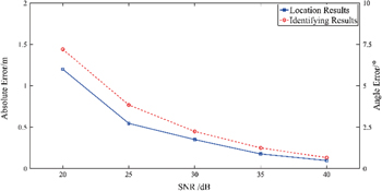
Fig. 8: Average recognition and localization errors with different SNR values.
Download figure:
Standard imageConclusion
In this study, the analytic expressions of the unit magnetic moment vector and the unit measurement point-source displacement vector were derived by using tensor geometric invariants. Following this, the inversion of the dipole was realized by combining the Frobenius norm. The proposed method is not affected by the attitudes, and the inversion result is unique. The method used to identify and locate the process employs analytical expressions; therefore, the calculations are computed in real time. The proposed method initially identifies the target; hence, the recognition results do not depend on the localization results. The simulation results verify the feasibility of the proposed method. The results show that the proposed method exhibits high accuracy. In theory, the location errors are limited to approximately 0.2%, and the identification errors are limited to 0.1°. The inversion effect of the proposed method is related to the conditional cosine, and the localization and recognition results exhibiting significant errors appear when the value of the conditional cosine is near to 1. Therefore, the conditional cosine should be less than 0.9 when determining the measurement point. However, the proposed method is susceptible to noise, and the inversion accuracy can be increased considerably by suppressing measurement noise.
The proposed method provides an alternative approach for the moving gradient tensor system to detect magnetic targets, and increases the means of magnetic anomaly detection technology. The concept of tensor geometric invariants can enrich magnetism theory. The cross-product of the intermediate eigenvectors between two measurement points in the same/opposite direction as the magnetic moment vector was found. This physical property provides a novel theory for magnetic target recognition. Our future research will focus on reducing the influence of noise in the proposed method.
Acknowledgments
This work was supported by the Fund for Shanxi "1331 Project" Key Innovative Research Team and partly by the Shanxi Scholarship Council of China (2017-092).