


Abstract
We report a critical behavior in the breakdown of an equal-load-sharing fiber bundle model at a dispersion  of the breaking threshold of the fibers. For
  , there is a finite probability Pb, that rupturing of the weakest fiber leads to the failure of the entire system. For
  ,
,  . At
. At  , with
  , where L is the size of the system. As
  , the relaxation time τ diverges obeying the finite-size scaling law:
  with
with  . At
. At  , the system fails, at the critical load, in avalanches (of rupturing fibers) of all sizes s following the distribution
  , with
  . We relate this critical behavior to the brittle to quasi-brittle transition in the model. For the local-load-sharing scheme, the system is found to be always brittle for sufficiently large system sizes.
Export citation and abstract BibTeX RIS
Introduction
Disorder, in the form of microcracks, dislocations, or grain boundaries, plays an extremely important role in determining the fracture properties of a material [1–3]. Disorders act as stress concentrators and nucleation centers for fracture. The cooperative effect of disorder primarily determines the brittle or ductile (quasi-brittle) nature of a fracture. If disorders act independently of each other, then the most vulnerable one will cause a fracture (the weakest link of the chain concept [4,5]). This gives rise to a brittle fracture since prior to fracture the system shows a linear elastic response to stress. On the other hand, the cooperative growth of cracks or cooperative motions of the defects like dislocations, grain boundaries etc. give rise to a quasi-brittle or ductile fracture [1–3]. Though in-depth analysis of the effect of defects in a stress field in general is extremely difficult, the consequence of disorder is aptly captured in the simple fiber bundle model of fracture. The model has received lots of attention over the years, as it reproduces various important telltale features of the complicated problem of fracture [6]. Here, we report, hitherto unexplored, a critical behavior in the model in terms of fluctuation of disorder in the system. The criticality is directly related to the brittle to quasi-brittle transition in the model and may have practical relevance in the context of such transitions in engineering brittle materials.
The role of disorder has been observed in some earlier studies. In [7,8], a brittle to ductile transition was observed in a random resistor network model. Brittle to quasi-brittle transition was studied in a continuum mechanical model with strain rate as driving parameter [9]. In the fiber bundle model also a brittle to quasi-brittle transition was observed earlier, where disorder was introduced as the fluctuation of elastic constants of individual fibers [10].
The fiber bundle model [6] consists essentially of fibers attached between two parallel bars. We consider here only Hookean fibers, though, in general, any stress-strain constitutive relation can be obeyed by them. The bars are pulled apart with a force which induces a stress on the fibers. Each fiber sustains a stress up to a threshold (chosen randomly from a distribution) beyond which it breaks irreversibly. Once a fiber breaks, the stress of the fiber is redistributed among other surviving fibers. If the stress is distributed equally among all the surviving fibers, the model is called the equal-load-sharing (ELS) model. This is a mean-field model which ignores any fluctuation in the stresses in fibers. In the local-load-sharing (LLS) model, the stress of the ruptured fiber is equally distributed on the nearest-neighboring intact fibers. This enhances the stress on the fibers and can cause a further failure of some fibers and the rupturing process continues. Otherwise, the system attains a stable state with few broken fibers, when a further increment of external load is required to make the fracture evolve. The evolution of fracture takes place in a series of avalanches (bursts) of rupturing of fibers as the stress is increased. The stress at which the failure of the entire system happens is termed as the critical stress or strength of the system.
In this letter, we study the fracture process in the fiber bundle model by tuning the width δ of the distribution  of the rupture thresholds x of the fibers. At low values of δ, the failure of the system occurs, typically, from the rupturing of a single fiber, the fiber with minimum breaking threshold xmin. On the other hand, for large values of δ, failure occurs through a series of stable states at different stress levels. As the applied load is raised, the system goes through these states in succession of avalanches of rupturing of fibers till the critical stress
  , when the remaining fraction nc of fibers ruptures, bringing to the failure of the entire system. We ask the following questions: i) Is there a critical value
  demarcating these two regimes? ii) What are the features of the transition at
  ? And iii) what are the manifestations of the transition on the macroscopic properties of the model? Lastly, the possible relevance of these features to the brittle to quasi-brittle transition observed in real materials is discussed.
Here, we present results for the uniform distribution of  over the window a to
  within the range [0,1]. For the uniform distribution, the existence of a
  has been mentioned before [11,12]. In ref. [11] a general expression of
  was derived for various types of threshold distributions. Our analytical calculation gives
  , in accordance with [11]. For
  , there is a finite probability Pb that rupturing of the weakest fiber leads to the failure of the entire system.
  as
as  . At
. At  , with
  , where L is the size of the system. We further show analytically that, as δ approaches
  , the relaxation time τ diverges as
  . Our numerical analysis gives the finite-size scaling form of the relaxation time. At
  , the evolution of fracture becomes extremely slow. We observe that the failure of the system occurs in a succession of avalanches of rupturing of fibers with time. The avalanche size distribution P(s) shows a scale-free behavior and follows:
  with
with  . These exponent values suggest that the critical behavior at
  is in a new universality class.
  is the transition point which demarcates the brittle phase (for
  ) from the quasi-brittle phase (for
  ) in the model.
Analytical calculations
Our analytical calculation is based on finding the number of surviving fibers at each stable phase of the model at different stress levels. At an applied stress  , the fraction
  of unbroken fibers is obtained by integrating the probability distribution p(x) from a to the redistributed stress
  . Inserting
  we get the expression for the fraction of the unbroken bond as

At the point of failure, the above equation admits only one solution. This gives the critical stress  and the critical fraction Uc of the fibers at the failure point:

If we start from a high δ-value and keep it lowering, Uc will increase and reaches 1 at  . On further lowering the δ-value, Uc will remain at unity. In the region
  , the analytical solutions are not valid. Inserting
  in eq. (2), we get the critical value
  below which the model shows an abrupt brittle-like fracture in the thermodynamic limit:
  . If a is 0, the abrupt fracture will never occur in the model and the system will always break in steps with increasing external stress. On the other hand, if a>0.5, the fracture will always be abrupt.
From the dynamics of the system, at the external stress  , the fraction
  of the unbroken fibers at time step
  can be expressed in terms of the fraction Ut at time t as [13]:

The rate of change of Ut is given by  . Combining this with eq. (3) we get

We solve the above equation for a slight deviation  of
of  from the breakdown point
  :
:  . We get an equation for
  with the solution close to
  (taking
  )
)

The change in the fraction of unbroken bonds is given by  , where A is a constant. The relaxation time has the form

The above behavior of τ shows clearly that the relaxation time diverges as δ approaches  .
.
Numerical results
To get a better insight of the nature of the transition, we have studied the transition numerically. For simplicity, we have considered the uniform distribution  with half-width δ and mean at 0.5. For such distribution
  (obtained from analytical calculation). Numerical results are obtained on averaging over 104 disorder configurations and for system sizes ranging from 102 to 106.
Figure 1 shows  for different values of applied stress
  and δ. Here, the black region denotes the system after complete failure
  and the yellow region represents the initial condition where all fibers are intact
  . The color gradient is the partially broken phase
  .
.  at the boundary of the black and yellow region denotes the critical stress
  . For
. For  ,
,  follows a straight line given by
  . This is the region where we go from the yellow to the black region by a single jump once the stress reaches the minimum threshold a of the fibers. For
  the critical stress deviates from the straight line and approaches to
  at
at  . In this region, fracture evolves through a series of partially broken stable phases at different levels of applied load.

Fig. 1: (Color online) The fraction of unbroken bonds  is plotted for different
  and δ. In the yellow region
  , while in the black region
  . The color gradient corresponds to partially broken configurations
  . At low δ-values, the system goes from the yellow to the black region at a critical stress with an abrupt fracture. For
  , the system goes from the yellow to the black region through a color gradient region signifying a gradual fracture at different stress levels. The boundary of the black region gives us the critical stress
  for the system.
Download figure:
Standard imageDue to the finite size of the system, even below  , global failure (rupture of all the fibers in the system) is not always obtained starting from the rupture of the weakest fiber. We determine Pb, the probability of global failure starting from the rupture of the weakest fiber, for various δ-values and for various system sizes (see fig. 2). For a particular system size L, we define the critical δ-value
  at which Pb goes to zero. It is quite clear that
  has a system size dependence and approaches to
  as
as  . We find that
  satisfies the finite-size scaling relation

where the exponent η has a value  and b is a constant. The error bar is determined from the least-square data fitting. It is to be noted that the fluctuation
  in the number of surviving fibers at the critical stress has been shown to scale as
  [14–16]. It is this fluctuation in Uc, which determines the fluctuation in critical δ-values for finite-size systems. This fluctuation should also tell us the probability Pb in a system of finite size.

Fig. 2: (Color online) Plot of Pb with δ for increasing system size values L = 100 (star), 500 (square), 1000 (open circle), 5000 (filled circle) and 10000 (triangle). For low δ, Pb is close to 1. As δ increases, Pb decreases till it goes to zero. This fall becomes more and more sharper as the system size is increased. In the inset variation of Pb with system size L is shown for  (star), 0.1666 (square) and 0.18 (open circle). For
  , Pb saturates, so that there is always a non-zero Pb value. For
  , Pb falls to zero exponentially fast. At
  ,
,  , with exponent
  .
.
Download figure:
Standard imageFigure 2(inset) presents the variation of Pb with system sizes in the neighborhood of  . For
. For  , Pb tends to saturate and there is always a non-zero probability of rupturing all the fibers starting from the single most vulnerable one. On the other hand, for
  , Pb falls off sharply to zero and the probability of having an abrupt fracture vanishes in the thermodynamic limit
  . At critical disorder Pb shows a scale-free behavior:

To establish the critical behavior at  , we study the relaxation time of the bundle at different δ-values with system sizes ranging from 104 to 105. To determine the relaxation time, we apply the minimum load that is needed to rupture the weakest fiber and the system is allowed to evolve (keeping the load constant) till it fails or reaches a stable state with partially broken bonds. The relaxation time is determined as the number of times the load is to be redistributed among the unbroken fibers over the evolution of the system. At a particular δ-value, for 103 configurations the maximum of these relaxation times is determined. Again over 103 configurations the average of these maximum values are obtained. We denote this average value as τ and use it to explain the critical behavior at
  . Figure 3 shows this variation of τ with δ for different system sizes ranging from 104 to 105. Previous studies have dealt with the behavior of the relaxation time close to the critical stress [16,17]. Here we have fixed the stress to be the minimum one and it approaches critical value at and below
  .
.

Fig. 3: (Color online) The relaxation time τ is plotted with δ for system sizes L = 10000 (star), 30000 (square), 50000 (hollow circle), 70000 (filled circle) and 100000 (triangle). In the inset the scaling of τ is shown. The scaling is done by plotting  against
  for the above-mentioned L values with
  and
and  .
.
Download figure:
Standard imageτ shows a maximum at  for the system size L. As L increases, the maximum value increases and the increment becomes sharper and sharper. Below
  the system experiences an abrupt failure within a few redistributing time steps starting from the rupture of the weakest fiber. On the other hand, for
  , due to a wide range of threshold values, the minimum stress corresponding to the weakest fiber is not sufficient to break all the fibers in the system. Starting from some initial rupturing of the fibers, the system comes to a stable configuration after few redistribution steps for the stress. In both these cases, τ is finite. At
  , τ diverges with the system size obeying a finite-size scaling:

where  . This system size effect of τ in the fiber bundle model has been observed before [18]. The scaling function
  assumes a constant value for x = 0 and
  for large x. Accordingly, at
  ,
,  , and close to
  ,
,

where  . The scaled τ is shown in the inset of fig. 3. The scaling is sensitive to the choice of the value of the exponent β, which determines the error bar of it by simply checking the collapse in the scaling. The value of the exponent
  is in agreement with our analytical result.
Figure 4 shows the avalanche size distribution P(s) vs. the avalanche size s. We start from applying a low load to the system, sufficient enough to rupture only the weakest fiber. Once a fiber is ruptured, the stress is redistributed among the remaining unbroken fibers. The breaking of fibers between any two consecutive stress redistribution steps constitutes an avalanche and the number of fibers broken gives the size of the avalanche. For  , the distribution tends to level off (up to a certain avalanche size) showing that big avalanches are equally probable. In this region, after few big avalanches, the system fails completely within few time steps. In the region
  , the distribution falls off very fast showing that, in this region, the system ceases to evolve after few small avalanches starting from the rupturing of the weakest fiber. At
  the distribution is a power law:

where the exponent is given as  .
.
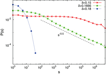
Fig. 4: (Color online) P(s) vs. s is plotted for  (star), 0.1666 (square) and 0.18 (filled circle). For
  , the distribution levels off. Since in this region the avalanches are uncorrelated, there is always a probability of having an avalanche of any size (even as big as the system size). For
  , P(s) falls to zero exponentially fast and there is no big avalanches found. At
  , P(s) falls in a power law behavior with exponent
Download figure:
Standard imageWe have also checked this critical behavior for the truncated Gaussian and power law distribution of the thresholds of the fibers. Within the error bar, the exponent values suggest universality.
Discussions
The ELS fiber bundle model is a mean-field model. Fracture in engineering samples deviates much from the ELS rule as the stress concentration around defects is a major concern in these systems. If one considers the simple LLS model, where the extra stress of a broken fiber is redistributed over the two surviving neighboring fibers, one still gets a  which demarcates an abrupt failure to the continuous failure with increasing stress. In LLS, however,
  depends on the system size L and increases with L. In the limit of a large system size, the failure is always brittle. Moreover, here at every step at best two fibers are broken because of the stress enhancement. The model does not show any critical behavior at
  . This is true in any dimensions. However, the above-mentioned LLS rule is the strongest LLS rule. One should study what happens if the stress of a broken fiber is allowed to relax over a large range as may be the case in experimental samples.
Fracture in quasi-brittle materials has tremendous technological relevance and as a result has received lots of attention in the past [1,19]. Brittle materials, like glass, ceramics, wood, do not show much deformation under stress and fracture abruptly [3]. Here, fracture is determined primarily by the nucleation of a vulnerable crack that spans through the system causing total failure. In heterogeneous materials, the quasi-brittle fracturing occurs by microcracking of the medium. It is characterized by complex temporal and spatial organizations of microcracks. This produces intermittency in the damage events and localization [19].
We find that the transition at  is marked by the divergence of relaxation time and fracture by creep. The creep phenomena and the avalanches in creep have been observed at the brittle to ductile transition point [20,21]. It will be worth investigating to what extent the transition, that is observed in the simple fiber bundle model, is related to the brittle to quasi-brittle or ductile transition in engineering materials.