Detection of Microbes in Ice Using Microfabricated Impedance Spectroscopy Sensors

Lauren B. Kaiser-Jackson; Markus Dieser; Matthew McGlennen; Albert E. Parker; Christine M. Foreman; Stephan Warnat

doi:10.1149/2754-2726/ad024d

The study of icy habitats on Earth provides an important analog for determining the likelihood of microbial life in extraterrestrial environments. The first goal of NASA's Astrobiology Roadmap defines a system as being habitable if it can sustain life by providing liquid water, conditions favorable for the assembly of complex organic molecules, and energy sources for metabolism.¹ Decades of studying microbial life in the Earth's cryosphere have not yet revealed a minimum temperature threshold for metabolism,^2,3 and genomic DNA and viable bacteria have been preserved in ancient ice and permafrost for hundreds of thousands to millions of years.^4–6 There are likely two factors that limit habitation at extreme low temperatures. (i) Absence of liquid water, if solvent conditions cannot be maintained,⁷ and (ii) vitrification, the temperature at which the cytoplasm transitions to a non-crystalline, amorphous solid.⁸ Planetary bodies such as Mars or icy Moons of Saturn and Jupiter could harbor cryopreserved microorganisms. In this search for life, studies have revealed that bacterial cells are physically located in the interstitial veins that exist in ice at grain boundaries and triple junctions,^9–11 supporting Price's hypothesis that ice veins provide a habitat for microbial cells.¹² At subzero temperatures, the presence of ice veins depends on the eutectic temperature of the brine solutions,^10,13–15 which can lower the freezing point to below −70 °C.¹⁶ The conditions that impact the habitability of ice are not thoroughly understood.

Existing tools such as nuclear magnetic resonance, Raman spectroscopy, or mass spectroscopy can be used to characterize the ice's microstructure, the ice vein network's chemical composition, and biological signals relevant to Earth analogs.^17–23 These techniques, however, are limited in field deployment due to physical and technical implementation or instrumentation requirements. Electrical conductivity measurements offer another way to characterize ice properties.²⁴ Ice is modeled as a solid electrolyte that can have electrical conduction caused by three main mechanisms: (i) The movement of charged protonic point defects formed by lattice-soluble impurities, a hypothesis originally developed by Jaccard.^24,25 (ii) Metallic impurities which can cause ion conduction through the ice lattice.²⁶ (iii) Freeze-concentration of impurities into ice veins (i.e., analogous to grain boundaries in solids).²⁴ In addition, the ice vein properties at low temperatures depend on salt concentrations. As observed in glacial ice, frozen ice veins with low salt concentrations (low available active water) can already form at −5 °C.²⁷ Also, vein width decreases with lower temperatures, further decreasing the electrical resistance in the veins. Interface polarization mechanisms²⁸ between the electrode and ice matrix are hypothesized to be a more efficient way to predict microbial presence in ice veins. All conductive systems contain dissolved free ions (in this study, microorganisms can also be considered charge carriers). Under the influence of an electric field, ions or microorganisms tend to move toward the electrode/sample interface, leading to the development of ionic double layers. The applied voltage drops rapidly in these layers, implying a large electrical polarization of the material and a near-absence of the electric field in the bulk sample at low frequencies. The resulting capacitance of these layers can dominate the signal at the lower frequencies, masking the relaxation of the bulk sample. This phenomenon is known as electrode polarization (EP). EP can present a major impediment to the interpretation of dielectric spectra. This is because the magnitude of EP depends on the electrical conductivity and temperature of the sample, the structure and composition of the electrodes, and even the roughness of the electrode surface. The characteristic length of the double layer ${\lambda }_{D}$ between the electrode and electrolyte is utilized as one method for EP description, in particular, ${\lambda }_{D}$ describes the thickness of the formed EP capacitor. The Gouy-Chapman model considers ion diffusion from the electrolyte to the electrode and the characteristic length is defined by the Debye–Hückel theory²⁸

$\begin{eqnarray}&&{\lambda }_{D}={\left({\epsilon }_{r}{\epsilon }_{0}{k}_{B}T\right)}^{0.5}{\left(2{e}^{2}\sum {n}_{i}\right)}^{-0.5}\end{eqnarray} \tag{ 1 }$

where ${\epsilon }_{r}$ is the relative permittivity of the medium, ${\epsilon }_{0}$ is the absolute permittivity of free space, ${k}_{B}$ is Boltzmann's constant, T is the temperature, e is the fundamental unit of charge, and $\sum {n}_{i}$ is the concentration of free ions and microorganisms. The polarization of cell membranes must be considered during electrochemical impedance spectroscopy (EIS) measurements if microbes are in the media.²⁹ Diffusion and cell membrane polarization may show different relaxation times (depending on cell media and type) and contribute polarization effects at different frequency regimes to the EIS response. Hence, EP could characterize the differences in the ice matrix, notably the presence of microbes in ice veins.

EIS is a common technique to characterize the electrical properties of solids and interface reactions between electrodes and electrical and/or ionic conductors. Evans pioneered EIS to characterize the dielectric properties of pure snow and ice samples,³⁰ and McGlennen et al. have recently shown characteristic impedance spectra for snow colonized by red algae.³¹ EIS allows the characterization of electrical conduction modes using a broad frequency regime and measures the complex impedance of a system by supplying a small electrical perturbation.³² The resulting measurement corresponds to electrochemical reactions occurring at the electrode's interface (i.e., in the present study the solid ice crystal and ice vein matrix). Measured complex impedance spectra can be presented graphically as a function of frequency (Bode-plot) or by the association of the imaginary (−Z'') to the real (Z') impedance (Nyquist-plot). Further, EIS spectra can be represented as electrical equivalent circuits (EECs), which describe reactions at the electrode/electrolyte interfaces, rather than physical and chemical models.³³ This interpretation allows an association of measured data to EEC elements and simplifies fitting algorithms of the recorded spectra. We present the use of microfabricated EIS sensors in tandem with fluorescence microscopy to detect microbes in icy environments. Effects of ice vein formation, abiotic impurities, temperature, and microbial impurities are investigated in a laboratory setting.

Experimental Design

Sensor design and fabrication

To maximize the chance of intercepting the heterogeneous microstructure of ice (i.e., network of ice veins and crystals) with the micro-interdigitated electrodes (μIDEs) upon freezing, the design of the sensor consists of four sets of μIDEs positioned in a perpendicular configuration (Supplemental Material, Fig. S1). Each μIDE is made up of five pairs of electrodes. The electrodes width and spacing were designed to be 7.5 μm to fit within ice veins and the microscope's field of view. Each device was equipped with two resistance temperature detector (RTD) sensors in a meander geometry (line width: 20 μm, 28 instances of repeating lines, total RTD length 115,360 μm, measurement area: 9.4 × 10⁶ μm²) as shown in (Supplemental Material, Fig. S1b)).

Sensors were fabricated using a similar protocol to McGlennen et al.³¹ A 100 mm Borofloat 33 dual side polish (DSP) wafer (University Wafer) was cleaned using a SEMITOOL spin rinse and dryer. The wafer was prepared for thin film deposition with O₂ plasma glow discharge at 600 W for 1 min in an Angstrom AMOD PVD evaporator. 10 nm titanium adhesion promoter, followed by 100 nm of gold, were deposited using electron-beam thermal evaporation in an Angstrom AMOD PVD evaporator. Gold was chosen as the electrode material due to its chemical inertness, biocompatibility, and previous successes in microbial detection during icy conditions.^31,34 The wafer was patterned with μIDE structures by standard photolithography techniques (i.e., spinning positive photoresist, exposure, development) and wet etching. Before lithography, the wafer was cleaned with O2 and Ar plasma at 600 W for 5 min in a PVA Tepla Ion. The wafer was spun coated with a 1.5 μm layer of positive photoresist (Microchem AZ1512HS) at 500 rpm for 10 s and 4000 rpm for 35 s. Next, the photoresist-coated wafer was soft baked on a hotplate for 1 min at 110 °C. Subsequently, the wafer was exposed with a light intensity of 11.75 mW cm⁻² for 4.0 s on a contact aligner (ABM contact aligner) for a total exposure of 47 mJ cm⁻². For development, the wafer was submerged in developer solution (MicroChem AZ300 MIF) for 1 min 15 s, rinsed with DIW (deionized water), and hard-baked for 2 min at 115 °C on a hotplate. Gold etching was performed at 22 °C by wafer submersion for 40 s in gold etchant (Transene Gold Etch TFA), followed by DIW rinse. Subsequently, titanium etching was performed at 22 °C by submerging the wafer in 40:1:1 H₂0:H₂0₂:HF for 12 s and DIW rinse. The photoresist was removed by spraying acetone, followed by 99% isopropanol, and drying with N₂ stream. Residual hard-baked photoresist was observed on the sensor μIDE structures and was removed by submerging the wafer in stripping solution (Microchem AZ400T Stripper) for 10 min at 75 °C. After etching, the nominal deposited metal layer thickness was 115 nm, calculated from the average step height from a profilometer scan (Ambios XP2 Profilometer) from four wafer regions. Using a dicing machine, the wafer was diced into individual sensors, 4.5 cm × 4.5 cm in size. The fabricated sensor structures (RTD and μIDE) are shown in Fig. 1.

**Figure 1.** (a) Microfabricated impedance spectroscopy sensor, (b) RTD sensor with a total resistance of 1871 Ω at 0 °C (Note: The image was stitched from two separate capture images.), (c) Micro-interdigitated electrode structures located in the center of the sensor.
Download figure:
Standard image High-resolution image

Ice crystal formation

A Linkam LTS420E-P temperature-controlled stage was mounted on a Nikon Eclipse E800 epi-fluorescent microscope and was used to form the ice matrix (i.e., ice veins and solid ice grains) on top of the μIDE structures. The stage allowed for precise temperature control (i.e., a maximum heating/cooling rate of 50 °C min⁻¹ and an accuracy of 0.01 °C) as low as −195 °C. After pipetting sample solutions onto the center of the microfabricated sensor, ice matrices were created by lowering the temperature by 50 °C min⁻¹ until the samples reached −25 °C. After 1.5 min, held at −25 °C, the stage was warmed to −10 °C at a rate of 10 °C min⁻¹ and held constant for another 1.5 min. The temperature was increased to −5 °C at a rate of 1 °C min⁻¹ and then to −0.5 °C at a rate of 0.5 °C min⁻¹. Liquid ice veins formed within the solid ice sample at temperatures between −0.9 °C and −0.4 °C. After liquid ice vein and solid ice grain formation, the temperature was decreased by 2 °C min⁻¹ and held constant at −10 °C for 1.5 min while impedance spectra were collected. Sequentially, the same decrease in temperature and holding was conducted for data collection at −20 and −25 °C. The complete temperature profile can be viewed in Supplemental Materials, Fig. S2. Ice veins were visually confirmed and imaged by transmitted and epi-fluorescent light using a 20X Nikon Plan Apo objective (NA 0.75, WD 1 mm). The stage lid was modified to allow the 1 mm working distance objective to capture clear images.

Sensor-stage set-up and temperature calibration

Electrical connections were established using 4 BNC (initialism of Bayonet Neill–Concelman) connectors. Each BNC terminal was attached to a positional tungsten needle-probe within the chamber, enabling the user to make electrical measurements on the sample. Each probe is equipped with a magnetic base that could be placed at any orientation on the metal plate within the stage. A secure connection between the HIOKI IM3536 lCR Meter (L inductive, C capacitive, R resistive) and the microfabricated sensor within the stage, was created by bending the gold-plated tip of the needle to contact the gold connection points surrounding the edge of the sensor (Fig. 2).

**Figure 2.** Linkam LTS420E-P temperature-controlled probe stage with the sensor positioned on the heating element and magnetic probes connecting the gold contact points. A: Positional tungsten needle-probe with magnetic base B: 2.5 mm aperture hole C: Electrical ports to connect cryo-stage and benchtop equipment D: Stage lid E: Sensor.
Download figure:
Standard image High-resolution image

To confirm that the sensor surface temperature matched the set temperature of the stage, resistance of the two RTD structures was measured. The sensor was placed on the heating and cooling element inside the Linkam LTS420E-P chamber. A 20 μl drop of Milli-Q water was dispensed onto the sensor, covering both meander structures, and a coverslip was placed on the Milli-Q water droplet. The stage was cooled to 0, −15, and −30 °C. The measurements of each meander structure's triplicate resistance were recorded at each temperature using a Hioki RM 3544–01 resistance meter. The measured resistance is the function of temperature and the temperature coefficient of the gold material. The linear temperature coefficient α is extracted using Eq. 2:

$\begin{eqnarray}&&\alpha =\left({\rm{R}}-{{\rm{R}}}_{0}\right){\left({{\rm{\Delta }}{\rm{TR}}}_{0}\right)}^{-1}\end{eqnarray} \tag{ 2 }$

with R the measured resistance at temperature T, R₀ the measured resistance at reference temperature T₀, and ΔT the temperature difference between T and T₀, respectively. The temperature calibration profile for both RTD structures can be seen in Supplemental Materials Fig. S3. An ohmic resistance R₀ of 1856 ± 21 Ω at 0 °C was measured, which agrees with the designed sensor geometries and indicates low electrical contact resistances in the set-up. The experimental linear temperature coefficient, derived from calibration for the Au material, agreed with the values reported in the literature and showed a stable and reliable environment suitable for studying electrical processes in ice across the investigated temperature range.³⁵ An α of 3,002 ± 9 ppm °C⁻¹ was estimated for the given instrumentation and sensor fabrication.³⁵

Test solutions

A fluorescent bead solution was used for modeling the behavior of abiotic impurities in ice veins and was prepared from stock (F8823, Invitrogen, Eugene, Oregon). One mL of the carboxylate-modified microsphere stock solution (1.0 μm, yellow-green fluorescent, emission maximum ∼515 nm, 3.6 × 10⁷ microspheres ml⁻¹) was centrifuged at 21,100 g for 3 min. Beads were washed in 1 ml of Milli-Q water and centrifuged at 21,100 g for 3 min. The final bead pellet was resuspended in a 176 μS cm⁻¹ conductivity solution (i.e., the control solution) (Eureka Water Probes, Austin, Texas). Electrical impedance was measured on samples containing ∼3.6 × 10⁵ microspheres ml⁻¹.

A microbe-doped solution was used for modeling the behavior of biotic impurities and was prepared using Escherichia coli HB101-GFP (green fluorescent protein³⁶). The E. coli HB101-GFP was grown in 1X TSB (Tryptic Soy Broth) in the presence of 100 μg ml⁻¹ ampicillin at 37 °C while shaken at 150 rpm for 16 h. Cells were harvested by centrifugation at 10,000 g for 5 min at 20 °C. The cell pellet was washed in Milli-Q water and centrifuged at 10,000 g for 5 min at 20 °C. The washed pellet was resuspended in the control 176 μS cm⁻¹ conductivity solution. Cells were stained with FM 4–64 (N-(3-Triethylammoniumpropyl)−4-(6-(4-(Diethylamino) Phenyl) Hexatrienyl) Pyridinium Dibromide) membrane for 1 h. The cell solution was centrifuged at 21,100 g for 3 min and washed in Milli-Q water. Final cell pellets were resuspended in 176 μS cm⁻¹ conductivity solution at a cell concentration of 10⁸ CFUs (colony-forming units) ml⁻¹ to create the E. coli solution (microbe experimental condition).

For experimentation, 20 μl drops of 176 μS cm⁻¹ conductivity solution doped with microspheres (fluorescent beads) or E. coli HB101-GFP were pipetted onto the sensor and covered with a 25 mm round cover glass (Celltreat Scientific Products). An unamended sample of 176 μS cm⁻¹ conductivity solution served as the control. The focus of the experimental design was to investigate impedance signals corresponding to the presence of microbes and inorganic impurities. Both E. coli and beads have a negative charge, and the change in EIS response may be related to the metabolism of E. coli on the sensor surface. As E. coli cells may attach to beads,³⁷ which would mask the contribution of biological or abiotic signals, solutions were not mixed in this work.

Impedance spectroscopy, data collection, and statistical analysis

Impedance spectra were collected at −10, −20, and −25 °C after ice matrix formation with the Hioki IM3536 lCR meter between 1 MHz − 4 Hz with a 100 mV RMS sine wave amplitude over 50 data points. At each temperature, data were collected from both the left-hand and right-hand μIDE structures, one being crossed by a ice vein and the other underneath an ice grain (Note: there are four total μIDE structures on the sensor, the top and bottom μIDE structures, seen in Fig. 1c, were not used to take measurements during experimentation). Data were collected for the control, bead, and E. coli HB101-GFP solutions. Figures 3a–3c show the varying stages in which the sensor electrode can interface with: (a) a liquid unfrozen sample, and after ice matrix formation, (b) an ice vein, and (c) a solid ice grain. Literature has concluded that ~90% of the electrical signal responses relate to the region above the electrodes, equivalent to ~twice the spacing between the electrodes.³⁸ Given the sensor geometry in this work, the measured signal captures changes about 15 μm into the ice matrix. Due to incomplete exclusion, some microbial cells are also anticipated to be present in ice grains. For scenarios b and c, triplicate measurements were collected (technical replicates).

**Figure 3.** Measurement configurations of sensor electrodes in contact with media and microorganisms (a), sample in liquid phase, prior to freezing (b), a liquid ice vein crosses the electrodes (c), a solid ice-grain crosses the electrodes. The shown electrical field lines penetrate through the test solutions and determine the impedance response. (d) Example of an electrical equivalent circuit (EEC) to model electrochemical processes at the ice/vein interface with a simulated spectrum.
Download figure:
Standard image High-resolution image

EIS allows the modeling of electrochemical processes using electrically equivalent circuits (EECs). Circuit elements were related to physical processes in the ice matrix (vein and no-vein), the interface reactions between sensor electrode and the ice matrix (vein and no-vein), and polarization mechanisms on the sensor surface,³³ as shown in Fig. 3d. However, established EEC models have not been applied or validated for the ice matrix described here. In particular, much needs to be learned about correlations between ice vein morphology and electrical resistance. We propose the following EEC to prove the methodology concept. Because the ice vein geometries are smaller than the sensor geometries, sensors span ice grains and ice vein simultaneously. Therefore, the bulk electrical conductivities of the solid ice grain and the ice vein were combined into R_Bulk. A parallel capacitor or constant phase element CPE 1 was added to simulate the microscopic electrode- ice matrix, including non-uniform surface and interface defects between the ice matrix and sensor electrode surface. A second R,CPE parallel configuration was added because ice matrices consist of multiple ice crystals divided by veins. Each of these vein-crystal interfaces adds additional resistive R_interface and capacitive CPE 2 contributions to the overall EEC. Electrode polarization (EP) by the media, beads, and E. coli was modeled in this initial EEC as a constant phase element CPE 3 in series with two R,CPE circuits. We evaluated the CPE 3 as an essential parameter to detect microbial presence in the ice veins because both beads and E. coli are negatively charged with a similar electrical potential of approximately −10 mV, however, we hypothesize the microbial metabolism can alter EP.

Model fitting was performed using RelaxIS 3.0 to fit electrical elements of an EEC to the impedance spectra. The software also estimated the accuracy of the model EEC. The model parameter of interest to be estimated and analyzed was CPE 3, which is related to EP (as shown in the introduction). After an EEC model was fit to the data from each technical replicate for each combination of temperature, veins, and beads/microorganisms, CPE 3 estimates were then analyzed by a linear mixed-effects model (LMM) using Minitab v.20. Fixed effects of interest were temperature, vein presence, bead/microbial presence, and the 2-way and 3-way interactions. Data were collected in blocks from different dates and 3 technical replicates of data were always collected for each experimental condition, the random effect in the model was the date on which experiments were performed. Residual plots were used to assess the normality and homogeneity of variance assumptions of the LMM.

Results

Impedance was measured at the selected experimental temperatures of −10, −20 and −25 °C across ice veins and solid ice grains (i.e., no veins) in control, fluorescent beads, and E. coli HB101-GFP solutions. The recorded impedance spectra of the different temperatures and solutions are presented in Nyquist plots created from EEC models in RelaxIS 3.0. An example of measured EIS spectrum of E. coli HB101-GFP and the fitted model CPE 3 fit parameters showed that the fit was accurate with relative error in a window of ±.01 (Supplemental Material, Fig. S4).

Microscopy images (Fig. 4) show an ice vein across the right-hand μIDE for the control conductivity solution (Fig. 4a), the left-hand μIDE for the fluorescent beads (Fig. 4b), and the right-hand μIDE for the microbial solution (Fig. 4c). During each experiment, measurements were taken on both the left- and right-hand μIDEs for direct comparison of the ice vein and ice grain (i.e., no veins) electrochemical properties.

**Figure 4.** Epifluorescence microscopy showing ice veins and grains formed on the EIS sensors (black structures) at −10 °C. (a) unamended control conductivity solution; (b) fluorescent beads (green); (c) fluorescent stained *E. coli* HB101-GFP (red). Beads and *E. coli* cells are largely found in ice veins.
Download figure:
Standard image High-resolution image

Fitted models for all experimental conditions are shown in Fig. 5. The first panel in each row shows the fitted model from each of the three technical replicates for the control solution (a-1), fluorescent beads (b-1), and E. coli HB101-GFP (c-1) with no-veins present across the sensor structures (μIDEs under an ice grain). For comparison, vein data (μIDEs under an ice vein) are shown in the right panel correspondingly.

**Figure 5.** Model fit to Nyquist data for control (row a), bead (row b), and *E. coli* HB101-GFP (row c) solutions for −10, −20, and −25 °C.
Download figure:
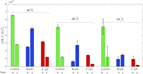
Standard image High-resolution image

A decrease in temperature led to a decrease in CPE 3 (increasing electrode polarization effect) for all experimental conditions (Fig. 6). Simultaneously, ice vein presence showed a reduced CPE 3 mean relative to the ice grain for the control and biotic solutions. The inverse trend was observed for the fluorescent bead solution; beads within the ice veins increased CPE 3 compared to solid ice grains.

**Figure 6.** Bar plot of the CPE 3 values. Tops of the bars indicate the mean, whiskers indicate the standard deviation of each group of experimental factors; vein presence (no/yes), solution (control conductivity solution, beads, *E. coli* HB101-GFP), and temperature. Note: The unit of CPE 3 is Siemens times seconds to the power of n with n system parameter.³²
Download figure:
Standard image High-resolution image

Changes in the CPE 3 indicated the presence of E. coli HB101-GFP cells in ice compared to frozen abiotic solutions (Fig. 6). The statistical model analyzed experimental effects on the CPE 3 value for all experimental conditions. It is important to note that the model had two large outliers, increasing the variance heteroscedastically across the different experimental conditions. The −10 °C, bead, no vein condition exhibited greater variance than the other experimental conditions due to one outlier. Comparatively, the −25 °C, control, no vein condition had two outliers per three technical replicates. There was no statistically significant variability among technical replicates.

Table I presents the grouping of CPE 3 means using the Tukey Method with 95% confidence. The Tukey Method creates confidence intervals for all possible differences of means at the same time, meaning it provides a side-by-side comparison of the mean of CPE 3 under all experimental conditions. If the confidence interval contains zero, no statistically significant difference between two means is indicated. The table displays the means of CPE 3 for each experimental condition which were distinct from one another. If the confidence interval of the difference of two experimental factors contains zero, meaning they are not statistically distinct from one another, then those two conditions will have the same grouping letter. For example, the CPE 3 of the control solution at −10 °C through an ice grain (i.e., no vein) is not discernable from the same solution under the same conditions at −20 °C nor −25 °C, they share the same grouping (a). However, when ice veins are present, the CPE 3 of the control solution at −10 °C is discernable from the same sample with no vein, aka they do not share the same grouping (grouping (a) vs grouping (c,d) respectively).

Table I. Grouping information using the Tukey Method and 95% confidence from Minitab v.20. Results describe all experimental conditions and the means calculated by data fitting in RelaxIS. Letters a—f explain means which are distinct from one another within a 95% confidence interval.

Temperatureveinstype	N	Mean of CPE 3	Grouping
−10 n control	3	6.570	a
−25 n control	3	5.110	a
−20 n control	3	5.083	a
−10 y beads	3	4.887	a	b
−10 n E. coli	3	3.207		b	c
−10 y control	3	2.840			c	d
−20 y beads	3	2.750			c	d
−10 n beads	3	2.537			c	d	e
−25 y beads	3	1.507				d	e	f
−20 n E. coli	3	1.473				d	e	f
−20 y control	3	1.237				d	e	f
−10 y E. coli	3	1.227				d	e	f
−25 y control	3	1.222				d	e	f
−25 n beads	3	0.959					e	f
−25 n E. coli	3	0.959					e	f
−20 n beads	3	0.652						f
−20 y E. coli	3	0.329						f
−25 y E. coli	3	0.192						f

In general, values of CPE 3 decreased alongside decreases in temperatures (Fig. 6). CPE 3 values were lower for both control and microbe solutions across all experimental conditions in the presence of ice veins relative to ice grains (i.e., no veins). There was a statistically significant difference between the liquid vein and solid ice grain conditions for the control and the microbe solution, across all measured temperatures (p-value < 0.001). However, the CPE 3 values displayed the inverse relationship for all bead solution combinations. The differences in the bead condition between the vein and no vein conditions were also statistically significant (p-value < 0.001). Notably, although the control and microbe solutions exhibited the same effects when comparing the vein to no vein condition, the significance of the change in CPE 3 was distinct (Table II). At all temperatures, the difference between the vein and no vein CPE 3 means for the control werelarger than for the microbe solution. The difference in the change of CPE 3 value between veins and no-veins in microbe solutions was statistically significant at −10 and −20 °C (p-value < 0.0005). However, the difference in the CPE 3 value for the same conditions at −25 °C was not statistically significant (p-value = 0.035). Therefore, the model exhibited a statistically significant difference between vein and no vein conditions across all both solutions at temperatures of −10 and −20 °C, but not at −25 °C.

Table II. The difference in the means of CPE 3 × 10⁸ in the presence of ice veins and ice grains for both the control and microbe solutions at all experimental temperatures. The p-value describes whether the difference in the vein and no vein means for the control and E. coli conditions are distinct at each experimental temperature.

Temperature [˚C]	Veins—no veins for control	Veins—no veins for E. coli	p-value
−25	−3.89	−0.767	0.035
−20	−3.85	−1.140	<0.0005
−10	−3.73	−1.980	<0.0005

This study did not quantify the absolute change in CPE 3 since the exact number of fluorescent beads or E. coli HB101 cells across sensor surfaces could not be determined. Therefore, the CPE 3 model only allows for a qualitative electrochemical interpretation of the samples and investigation of the statistical significance of effects due to the experimental conditions. Additionally, salinity affects the size of liquid water inclusions and aspects of microbial life by influencing viscosity, motility, diffusion, and metabolic rates. In contrast to water, ice crystals are poor solvents and reject most foreign substances. Research suggests a heterogeneous distribution of solutes in these liquid channels in ice.¹⁴ The concentration of both organic and inorganic compounds of water inclusions in ice (e.g. NaCl, MgSO₄, CaCl, KCl, MgCl) would require more detailed analytical characterization using advanced high-resolution microscopy such as Raman spectroscopy. Since the exact composition and salinity of ice habitats is unknown, we selected a conductivity calibration solution of 176 μS cm⁻¹ for proof of concept of microbial detection in ice using EIS . Other EEC parameters, as shown in figure 3. were analyzed, box-plots analogous to fig. 6 are shown in the Supplemental Materials (Figs. S6–S9), and physical interpretation identified that CPE 3 is an efficient way to detect microbial presence in ice veins.

Discussion

This study applied a novel sensor and experimental design to study ice vein compositions (i.e., the presence of microbes or beads) using microfabricated sensors and impedance spectroscopy. Fitting algorithms of electrochemical equivalent circuits were utilized to confirm statistically significant differentiation of the composition of the ice matrix. The constant phase element CPE 3, which considers the electrode polarization mechanisms of the beads and microbes, was used in the statistical algorithms. By quantitatively confirming distinct electrochemical behaviors in the presence or absence of microbes and ice veins, we show that the use of microfabricated EIS sensors has the potential to conduct real-time Astrobiological exploration.

The LMM calculated for CPE 3 depicted differentiable means between ice veins and solid ice grains for all experimental conditions and highlighted opposing electrochemical behavior of ice doped with microbes and ice doped with beads. Lowered temperatures related to a decrease in the double layer, ${\lambda }_{D}$ as seen in Eq. 1. As the temperature decreased, smaller values of CPE 3 were observed, indicating a reduction in EP. This observation confirms that the EIS sensor can detect this phenomenon.

Comparing the CPE 3 values of each media type (control, bead, E. coli HB101-GFP) against the vein or no-vein measurement indicated that EIS sensors could detect microbes in ice matrices. CPE 3 values decreased in the presence of ice veins relative to the solid ice grains in the control solutions (Fig. 6). During freezing and ice grain formation, salts into solution.²⁴ With decreasing temperatures, vein sizes become smaller (i.e., less liquid water), while salts become increasingly concentrated. Ultimately, liquid ice veins will freeze solid upon reaching their eutectic temperature. This freeze concentration of ions $\sum {\bf{v}}{{\boldsymbol{n}}}_{{\boldsymbol{i}}}$ will trigger a decrease in the characteristic length ${\lambda }_{{\boldsymbol{D}}}$ and EP as described in Eq. 1. The freezing also differentiated cells and beads primarily into the ice-vein (Fig. 4). Although both solution displayed the same trend in their CPE 3 response, the difference in CPE 3 between the vein and no vein conditions for the solution containing microbes was much smaller than that for the control solution. This is key to the ability to detect the differences in ice with or without microbial presence in the liquid veins. These discrepancy in CPE 3 values between the control and microbe solutions suggest that cells present in ice grains or veins reduced EP by transferring electrons between the cell membrane and the electrode that desribes microbial metabolic processes.^32,39 On the other hand, the bead-doped solution displayed an increase of CPE 3 for all ice vein conditions relative to the ice grain (Fig. 6). Beads are electrical insulators that block charge transfer inside ice veins near the electrodes. It is assumed that beads located at the electrode-ice vein interface increase the length of the Debye layer, which increases CPE 3 and consequently EP. It should be noted that not all solid impurities were displaced into the liquid veins and some became encapsulated by solid ice grains (e.g., Fig. 3b). However, the μIDE structure located directly underneath veins did not measure those impurities.

Regarding astrobiological uses, we currently have a success rate of approximately 25% for forming an ice vein across one μIDE and no vein across the other simultaneously. The technology readiness level (TRL) of our technology is currently low. We anticipate that future work for astrobiology applications requires the integration of the sensors on a Rover-like robot. The sensor could be placed on the icy surface, allowing freezing to occur over the sensor with a defined pressure to detect possible microbial life ice microstructure. The anticipated high microbial concentrations in ice veins, if the analog to the Earth habitat is true, will statistically increase the possible detection rate.

Conclusions

The present study established that μIDE-sensors in combination with fitting of an electrochemically equivalent circuit model to Nyquist data, are useful tools to detect electrochemically distinct signals between E. coli HB101-GFP doped and abiotic solutions in complex ice matrices. The results relied on the visual confirmation of ice veins spanning the μIDEs. General abiotic reference impedance spectra are needed to identify microbial signals without prior knowledge of the ice matrices. Nevertheless, this result informs future investigations of microorganism presence in icy habitats on Earth as an analog for icy extraterrestrial bodies. This technology can also be used to prepare future icy world exploration by furthering understanding of electrochemical behaviors in subzero environments, such as brine solutions in ice veins at significantly colder temperatures.

Acknowledgments

This work was performed in part at the Montana Nanotechnology Facility, a member of the National Nanotechnology Coordinated Infrastructure (NNCI), which is supported by the National Science Foundation (Grant# ECCS-2025391). Imaging was made possible by the Center for Biofilm Engineering Imaging Facility at Montana State University, which is supported by funding from the National Science Foundation MRI Program (2018562), the M. J. Murdock Charitable Trust (202016116), and the US Department of Defense (77369LSRIP). The work was funded by the National Science Foundation (1760616, 2037963) and the NASA Exobiology program (80NSSC18K0814).

Detection of Microbes in Ice Using Microfabricated Impedance Spectroscopy Sensors

Article metrics

Author e-mails

Author affiliations

ORCID iDs

Dates

Abstract

Highlights