Abstract
Parameter sensitivity analysis of mechanistic battery models has the power to quantify the individual and joint effects of parameters on the performance of lithium-ion cells. This information can be beneficial for industrial cell designs, cell testing, and battery management system (BMS) configurations. The numerical quantification of these parameter sensitivities, however, is challenging in terms of computational costs and is an active field of research. In this paper, based on a 3D multiphysics model, we conduct a global sensitivity analysis for the utilizable cell discharge capacity and the maximum cell temperature at the discharge rate of 1C. The least angle regression version of the polynomial chaos expansion (PCE) concept has been identified as an optimal trade-off between approximation power and computational complexity. As a result, the sensitivities of all parameters in the 3D multiphysics model were studied using a hierarchical design and a stepwise design. We conclude that the cell discharge capacity and the thermal behavior at 1C discharge are most sensitive to the electrode parameters and their pore structure. The results reveal different dependencies and lead to new insights for cell design and operation.
Export citation and abstract BibTeX RIS

This is an open access article distributed under the terms of the Creative Commons Attribution 4.0 License (CC BY, http://creativecommons.org/licenses/by/4.0/), which permits unrestricted reuse of the work in any medium, provided the original work is properly cited.
Lithium-ion batteries (LiBs) are widely used in automotive and aeronautics but require improvement regarding high energy and high power.1–5 This need motivates the evolutionary development of novel electrode materials and innovation of cell designs in battery research and engineering.6–8 Typically, physics-based models provide much assistance in cell design, analysis of battery mechanisms, and solutions for safety issues. They are crucial as well to give insight with the effect of changes with production processes or cell performance.9 Detailed analyses and characterizations of multiphysics processes in LiBs can be carried out via Newman's pseudo two-dimensional (P2D) model10,11 or multi-dimensional multiphysics (MDMP) models.12,13 Recently, various MDMP models have been developed for detailed simulations accounting for battery heterogeneity and nonlinearity within real cell components and geometry,14–16 up to the microscopic particle properties.17 As high dimensional MDMP models can simulate and predict battery performance under realistic operating conditions, their results are much closer to reality, but with a high computational cost. At the same time, MDMP models are directly related to and determined by their parameters, including design and physical properties. An intensive study of these parameter sensitivities is essential for a thorough understanding and better optimization of battery performance. Sensitivity analysis characterizes the relation between parameters and model responses;18 thus, it provides valuable information regarding parameter identifiability, as well as feasibility studies of desired battery performances. However, as especially high dimensional models are computationally demanding, an efficient parameter sensitivity analysis of the MDMP model is necessary and beneficial for advancing utilization in the development and design of LiBs.
Various parameter sensitivity studies employed in LiB research are available in the literature,19,20 e.g., to figure out the effects of parameter variation on thermal and electrochemical behavior. Zhang et al.19 used the parameter sensitivities calculated from model simulations to categorize the model parameters with different sensitivity levels and improved the quality of parameter identification based on the stepwise design of experiments for each parameter cluster. Vazquez-Arenas et al.21 indicated that parameter sensitivities provide precise information for predicting and optimizing a model as they show whether parameters have significant impacts on the variation of the model output or not. In most studies, however, the sensitivity analysis of Li-ion batteries frequently relies on scenario analysis19,21 and local sensitivity studies,20,22 which investigate only minor parameter changes, i.e., exploring narrow ranges of the entire parameter space. This could lead to an inevitable loss of information and biased results, and it does not reveal critical parameter interactions. In first studies, we used GSA to identify the parameter uncertainties of an electrochemical-mechanical model for solid-electrolyte interphase evolution, based on a single particle model.23 GSA, to the best of the authors' knowledge, has not yet been applied to large-scale multiphysics Li-ion battery model, can be a valuable tool in LiB research. The implementation, however, is challenging because of the CPU-intensive 3D model and its vast number of parameters. In this paper, the focus is on the efficient implementation of a global sensitivity analysis framework of the 3D battery model. Figure 1 shows the overall architecture of the proposed concept and potential applications. The framework provides sufficient quantitative information about parameter ranking, which effectively reduces the need for experimental testing stemming from a large number of parameters. In the framework, a CPU-friendly GSA calculation method is obtained as explained in the following.
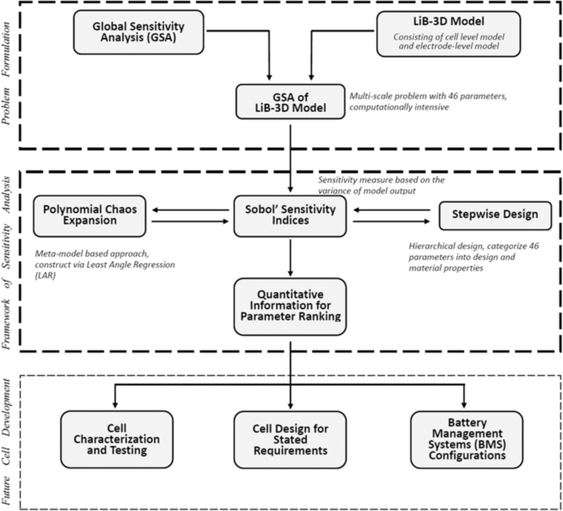
Figure 1. Structure diagram for global sensitivity analysis of 3D multiphysics model for Li-ion batteries (LiB-3D model). The first two frames are the focus of this work, and the third frame describes possible future applications of the results.
Global sensitivity analysis has been exploited and implemented in different research fields over the last two decades.24–27 It quantifies the variation in the model response in the entire parameter domain and comprehensively analyzes individual and joint effects of parameter variations. In the literature, various methods for global sensitivity analysis exist, e.g., derivative-based global sensitivity methods,28 non-parametric concepts,29 variance-based approaches,30 and density-based methods.31 As Li-ion battery models include highly nonlinear physicochemical phenomena, the non-parametric methods specified for linear models are not suitable here. The sensitivity indicators calculated with the derivative-based method and the density-based method, in turn, are not easy to interpret in general or to connect to the total variation of the model response. Thus, the variance-based method, i.e., the Sobol' sensitivity indexes,30 is the standard method in global sensitivity analysis and the best option for our Li-ion battery model. The Sobol' sensitivity indexes are constructed with statistical terms, i.e., the variance and partial variances of the model output. The required statistics are typically derived via Monte Carlo (MC) simulations.32 However, MC simulations require a significant number of model evaluations which need to cover the entire parameter space to provide a reliable estimation of the statistical quantities. As a single evaluation of our 3D battery model is CPU-intensive, the demand for computing sensitivities via MC simulations might become prohibitive. To balance the computational costs, polynomial chaos expansion (PCE)33 as an efficient method for sensitivity analysis is an attractive alternative and the method of choice in this paper. However, the number of model evaluations required for constructing the PCE model increases dramatically with the number of model parameters considered; i.e., PCE suffers from the curse of dimensionality.34 Thus, the PCE model is parametrized by the least angle regression (LAR) method35,36 which typically ensures affordable computational costs. Another problem also arises with utilizing LAR: Parameters with low sensitivities will be concealed and cannot be analyzed for large-scale systems. To avoid this problem, the parameters of the 3D multiphysics model are categorized into two groups, i.e., design and material properties, followed by an analysis of each group.
The paper is constructed as follows. In the first section, a 3D multiphysics model and a stepwise design of the global sensitivity analysis are introduced. Then, a systematic analysis is presented for the impact of the 46 model parameters on the discharge capacity and the maximum cell temperature that reveals the critical parameters and the parameter dependencies. The derived results are discussed in the context of LiB design and electrode configurations, respectively.
3D Multiphysics Model
The applied 3D multiphysics model consists of a 3D thermal-electric submodel combined with a 1D electrochemical submodel. The hierarchical framework and model schematics are illustrated in Figure 2 and are explained in detail in the following.
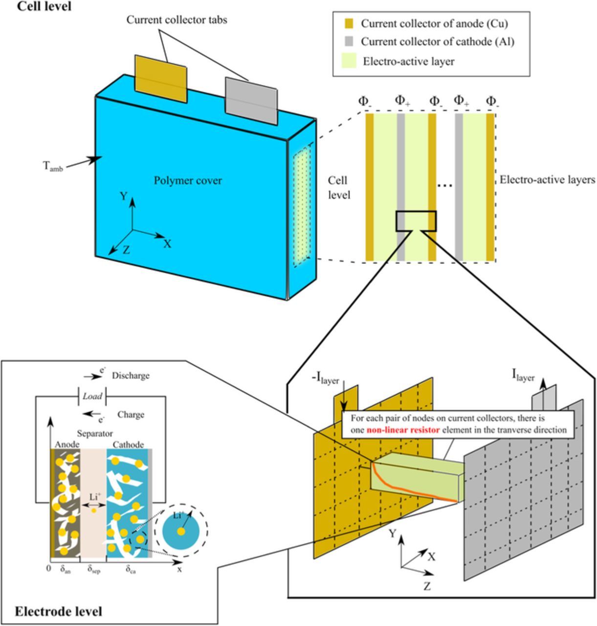
Figure 2. Scheme of the 3D multiphysics model for a 10 Ah pouch cell. The model consists of two submodels. The cell-level model describes the thermal-electric behavior in 3D domains, and the electrode-level model simulates the local electrochemical performance in 1D.
Electrode-level model
The electrode-level model is used to describe the local electrochemical performance of one electro-active element in a single cell as shown in Figure 2. Its domains include an anode, a cathode, and a separator. Two current collectors are defined as boundaries. The intercalation reactions occurring at the electrolyte-electrode interfaces are denoted by
![Equation ([1])](https://content.cld.iop.org/journals/1945-7111/165/7/A1169/revision1/d0001.gif)
where the backward and forward reactions represent the discharge and charge processes, respectively. LiyMO2 represents the functional metallic oxide material for cathodes. The electrode-level model is based on Newman's P2D model11,37,38 and is simplified with the volume average method.39,40 Here, the lumped pore-wall flux  can be defined as equal to
![Equation ([2])](https://content.cld.iop.org/journals/1945-7111/165/7/A1169/revision1/d0002.gif)
where δi is the electrode thickness, ai is the specific area of the electrode, F is the Faraday constant, ix, i is the current density on the current collector, flowing in or out of the electro-active layer and jx, i is the intercalation reaction current density. By using this lumped variable  , the lithium intercalation and deintercalation processes in active particles are assumed to be spatially independent along the x direction in good accordance with the full-order model.41 In this way, the solid diffusion process can be derived analytically.42 The electrochemical kinetics can be expressed via the Butler-Volmer equation as
![Equation ([3])](https://content.cld.iop.org/journals/1945-7111/165/7/A1169/revision1/d0003.gif)
![Equation ([4])](https://content.cld.iop.org/journals/1945-7111/165/7/A1169/revision1/d0004.gif)
where Ru is the ideal gas constant, T is the operating temperature, and αa, i and αc, i are the charge transfer coefficients. Equation 4 denotes the overpotential ηi on the electrode which is defined as the deviation between the difference between the potential in solid and solution phases and the open circuit potential (OCP). Following the model simplification,41 we define ηca = ηca(L) and ηan = ηan(0) to evaluate  according to Equations 2 and 3. i0, i is the exchange current density which is given by
![Equation ([5])](https://content.cld.iop.org/journals/1945-7111/165/7/A1169/revision1/d0005.gif)
where k0, i is the kinetic rate coefficient, and ce is the salt concentration of the electrolyte at the electrolyte–electrode interfaces. On the cathode, ce, ca = ce(L) and when on the anode, it denotes ce, an = ce(0). cs, surf, i is the lithium concentration at the surface of the active solid particles, and cs, max, i denotes the maximum lithium concentration in active particles. For the derivation of cs, surf, i, we refer to Guo's work.42 When assuming αa, i = αc, i = 0.5, most of the charge and mass conservation equations in the full-order P2D model can be solved analytically.43 Based on the approximations and simplifications above, the full-order P2D model results in our electrode-level model. The governing equations of the electrode-level model are listed in Table I.
Table I. Governing equations of the electrode-level model.
| Cathode and anode Dependent variables with i ∈ {an, ca} | Equation |
|---|---|
| cs, surf, i(t) |   |
| λn − tan λn = 0, n = 1, 2, 3, ... | |
| ηi(t) |  |
| Φs, i(x, t) |  |
| σeffi∇Φs, i|x = 0, L = −ix | |
| Φs, i|x = 0 = Φ− | |
| Φe(x, t) |  |
| ∇Φe|x = 0, L = 0 | |
| ce(x, t) |  |
| Deffe, i∇ce|x = 0, L = 0 with L = δan + δsep + δca | |
| Separator | |
| Φe(x, t) |  |
 |
|
 |
|
| ce(x, t) |  |
 |
|
 |
Cell-level model
The cell-level model simulates the cell temperature T and a pair of electric potentials, Φ+ and Φ−, on the current collectors and tabs. At the cell level, there are six computational domains, including the electro-active layers, two current collectors, two electrode tabs, and the protective polymer cover as shown in Figure 2. The thermal and electric properties of each cell component are considered to be anisotropic between the XY plane and the Z direction. The energy conservation of the cell yields
![Equation ([6])](https://content.cld.iop.org/journals/1945-7111/165/7/A1169/revision1/d0006.gif)
where material density ρ, specific heat capacity Cp, and thermal conductivity k are attributed to every domain. The volumetric heat sources  is defined in the electro-active layers and is evaluated by the electrode-level model as follows44
![Equation ([7])](https://content.cld.iop.org/journals/1945-7111/165/7/A1169/revision1/d0007.gif)
![Equation ([8])](https://content.cld.iop.org/journals/1945-7111/165/7/A1169/revision1/d0008.gif)
![Equation ([9])](https://content.cld.iop.org/journals/1945-7111/165/7/A1169/revision1/d0009.gif)
![Equation ([10])](https://content.cld.iop.org/journals/1945-7111/165/7/A1169/revision1/d0010.gif)
where  is the reaction heat,
  is the joule heat, and
  is the entropy change of the electrodes. The boundary conditions are on the surfaces of the polymer cover domains and tabs with the air convection are
![Equation ([11])](https://content.cld.iop.org/journals/1945-7111/165/7/A1169/revision1/d0011.gif)
where  is the normal unit vector, and βh is the heat transfer coefficient between the cell and the environment. The ambient temperature Tamb is assumed to be constant. The charge conservation of the cell on the current collectors and tabs follows the Poisson equation,
![Equation ([12])](https://content.cld.iop.org/journals/1945-7111/165/7/A1169/revision1/d0012.gif)
where σj is the electric conductivity of the current collector, and iZ, is the volumetric current density between the electro-active layers and the current collectors. On the current collectors,  , denoting the extra volumetric current density on electro-active layers, and on tabs, iZ, j = 0. The boundary conditions on the tabs read as
![Equation ([13])](https://content.cld.iop.org/journals/1945-7111/165/7/A1169/revision1/d0013.gif)
and the tab of the negative electrode is defined as the ground electric potential,
![Equation ([14])](https://content.cld.iop.org/journals/1945-7111/165/7/A1169/revision1/d0014.gif)
Figure 2 illustrates that the electric conduction of the electro-active layers in the Z direction is assumed to be a nonlinear resistor network.45 The local resistance Rnode can be evaluated with the electrode-level model with
![Equation ([15])](https://content.cld.iop.org/journals/1945-7111/165/7/A1169/revision1/d0015.gif)
where Inode is the local current through an elemental resistor. Φ+, node and Φ−, node are the local electric potentials on the nodes of the cathode and anode current collectors, respectively. The local current Inode can be evaluated with
![Equation ([16])](https://content.cld.iop.org/journals/1945-7111/165/7/A1169/revision1/d0016.gif)
where Nelem is the total number of nodes of a meshed current collector. Then we define the difference, Φ+, node − Φ−, node, as an inter-level variable, which couples the electrode-level model with the cell-level model. The resulting coupling expression reads as
![Equation ([17])](https://content.cld.iop.org/journals/1945-7111/165/7/A1169/revision1/d0017.gif)
Parameter set and simulation studies
The set of physical parameters for a 10 Ah pouch cell (anode: graphite, cathode: NMC) that is 120 mm wide × 99 mm high is given in Tables II and III. In this paper, βh is set to 10 W/m2 · K, referred to the natural convection value.46 The thickness of the cell is varied and determined by specified parameter ranges. All parameters used to initialize the model are set to the literature values taken from Guo et al.15 The kinetic coefficients k0, i, the solid diffusion coefficients Ds, i, and the diffusion coefficient in the electrolyte De are denoted as temperature-dependent functions in the Arrhenius type. The ionic conductivity κ is expressed as a temperature-dependent empirical equation. Parameters not listed in Tables II and III are given in the Tables AI and AII. The parameter ranges are defined from the Sauer group's results.47 Technically, Gaussian and uniform distributions are used to describe the variability of the parameters and provide the key information for global parameter sensitivities as described in the following.
Table AI. Cell geometry data.
| Description | Value, mm |
|---|---|
| Thickness of polymer cover | 1.12 |
| Thickness of clamps and tabs | 0.1 |
| Width of clamps and tabs | 22 |
| Height of clamps | 7 |
| Distance between cell side and clamps | 15 |
| Height of tabs | 10 |
| Thickness of anode current collector | 0.011 |
| Thickness of cathode current collector | 0.016 |
Table AII. Physical constants.
| Ideal gas constant, Ru(J/mol · K) | 8.3145 |
|---|---|
| Faraday constant, F(C/mol) | 96487 |
| Reference temperature, Tref, (K) | 298.15 |
Table II. Electrochemical properties and geometry data for 1D electrochemical model in global sensitivity analysis.
| Parameters | Anode | Range | Separator | Range | Cathode | Range |
|---|---|---|---|---|---|---|
| Design parameters for cell structure | ||||||
| Particle radius, R(μm) | 12.5a,u | 7–13a,u | 5a,u | 3–7a,u | ||
| Thickness, δ(μm) | 91.2c,u | 25c,u | 20–30c,u | 60c,u | 30–100c,u | |
Porosity,  |
0.4a,u | 0.3–0.5a,u | 0.4a,u | 0.4–0.6a,u | 0.4a,u | 0.3–0.5a,u |
| Volume fraction of binder, b |
0.19a,u | 0.01–0.2a,u | 0.09a,u | 0.01–0.2a,u | ||
| Bruggeman factor, b | 2a,u | 1.5–4a,u | 2a,u | 1.5–4a,u | 2a,u | 1.5–4a,u |
| Specific surface area, a(m2/m3) |  |
 |
||||
| Thickness of current collector, δcc(μm) | 11a,g | 50% a,g | 16a,g | 50%a,g | ||
| Solid phase | ||||||
| Specific capacity, ρe(mAh/g) | 368c,u | 178c,u | 153–178c,u | |||
| Maximum Li+ concentration, cs, max(mol/m3) | 28700a | 36224a | ||||
| Initial Li+ concentration, cs, in(mol/m3) | 26130 | 3984.6 | ||||
| Solid diffusion coefficient, Ds(m2/s) | 9.0 × 10⁻¹⁴ a,b,u | 3.0 × 10⁻¹⁵– 3.0 × 10⁻¹³ a,b,u | 3.0 × 10⁻¹⁵ a,b,u | 10−16–10−14 a,b,u | ||
| Electric conductivity, σ, (S/m) | 13.991a,b,u | 10.571– 17.411a,b,u | 23.797a,b,u | 19.370– 28.224a,b,u | ||
| Reference kinetic coefficient, k0(m2.5/mol0.5 · s) | 7.733 × 10⁻¹⁰ a,c,u | 10−11–10−9 a,c,u | 4.966 × 10⁻¹¹ a,c,u | 10−12–10−10a,c,u | ||
| Activation energy of solid diffusion, ED(kJ/mol) | 35a,b,u | 35–40.8a,b,u | 40a,b,u | 30–80a,b,u | ||
| Activation energy of reference kinetic coefficient, Er(kJ/mol) | 53.4a,b,u | 45–60a,b,u | 30a,b,u | 30–50a,b,u | ||
| Transfer coefficient, α | 0.5 | 0.5 | ||||
| Solution phase | ||||||
| Initial electrolyte concentration, ce, 0(mol/m3) | 1200a,g | 10%a,g | ||||
| Transference number, t+ | 0.363a | 10%a | ||||
| Activation energy of electrolyte diffusion, Ee(kJ/mol) | 17.120a,b,u | 16.99– 17.25a,b,u | ||||
aRef. 12. bRef. 36. cEstimated: based on Ref. 46. gGaussian distribution, value represents standard deviation. uUniform distribution. Note: Percentage number represents the standard deviation from the expected value, and all physical constants are listed in Appendix A.
Table III. Thermal properties of cell components for global sensitivity analysis.
| Density | Specific heat | Thermal conductivity | ||||
|---|---|---|---|---|---|---|
| Component | ρ(g/cm3) | Range | capacity Cp(J/g · K) | Range | k(W/K · m2) | Range |
| Electro-active layers | ||||||
| Cathode | 4.8c | 4.75–4.85u | 1.106c | 10%g | 1.0c | 10%g |
| Anode | 2.09c | 2.09–2.28u | 1.095c | 10%g | 1.0c | 10%g |
| Binder | 1.78c | 10%g | 1.3c | 10%g | 1.0c | 10%g |
| Separator | 0.9c | 10%g | 1.883c | 10%g | 0.5c | 10%g |
| Electrolyte | 1.2c | 10%g | 1.545c | 10%g | 0.5c | 10%g |
| Copper current collectora | 8.9 | 0.383 | 401 | |||
| Aluminum current collectora | 2.7 | 0.896 | 237 | |||
| Clamp and tab Coppera | 8.9 | 0.383 | 401 | |||
| Aluminuma | 2.7 | 0.896 | 237 | |||
| Polymer cover | 1.95c | 10%g | 0.9c | 10%g | 0.12c | 10%g |
aRef. 10. cEstimated: based on Ref. 50–52. gGaussian distribution; value represents standard deviation. uUniform distribution. Note: Percentage number represents the standard deviation from expected value.
It is noticed that the anode thickness δan is not considered to be an identified parameter in Table II due to an assumption of the design capacity in the manufacturing process according to:
![Equation ([18])](https://content.cld.iop.org/journals/1945-7111/165/7/A1169/revision1/d0018.gif)
The reason that we choose a specific capacity ratio between cathode and anode in Equation 18 is to prevent lithium plating, resulting from the overpolarization at the anodes under accidental overcharging, adverse charging conditions after manufacturing, and this is always a self-defined standard in industry.48 Based on Equation 18, we can derive a relationship between the cathode and anode thickness as:
![Equation ([19])](https://content.cld.iop.org/journals/1945-7111/165/7/A1169/revision1/d0019.gif)
Electro-active layer numbers Nlayer can be described as
![Equation ([20])](https://content.cld.iop.org/journals/1945-7111/165/7/A1169/revision1/d0020.gif)
Thus, according to Equations 19 and 20, Nlayer, δan and δca has correlated equations. It means both Nlayer and δan will change as well, when we change δca with a fixed design capacity of large-format pouch cell with parallel layers, for example 10Ah. Meanwhile, we motivate to include manufacturing factors, such as the capacity balancing consideration, we keep this relationship in the following GSA. Therefore, in the following, we only choose δca as a parameter, since it can represent the impacts of Nlayer and δan.
In this work, we simulate a 1C discharge process with an initial and ambient temperature of 25°C. The cell discharge capacity and the local maximum cell temperature are defined as the outputs in the global sensitivity analysis. In the following we use a categorization strategy for the investigated parameter sets referred to the identification results of Zhang et al.,19 In detail, we categorize them regarding electrode and cell production relevant parameters and physical parameters. The cell-level model is implemented by ANSYS APDL 15.0, and the electrode-level model is executed by MATLAB with the SUNDIALS TB solver.49 All simulation studies are run parallelized on three PCs with an 8-core I7–2600 processor with 16GB memory.
Parameter Sensitivity Analysis
Global sensitivity analysis (Sobol' indexes)
The parameter global sensitivities are quantified by analyzing the variation of the quantity of interest (QoI) on the entire parameter space through different methods. The Sobol' indexes,30 well-defined and robust measures for GSA, are the percentages of the total variance of the QoI related to a single parameter or parameter interaction. For a more detailed illustration, the total variance of the QoI, e.g., the discharge capacity or the maximum cell temperature, is decomposed as:30
![Equation ([21])](https://content.cld.iop.org/journals/1945-7111/165/7/A1169/revision1/d0021.gif)
This is a unique decomposition derived based on the assumption of independence for the parameters, which is the case in this work. V(QoI) is the total variance of the QoI, and the summands,  with npbeing the number of parameters, are partial variances which are defined as variances of conditional expectations with respect to certain parameters and read as:
![Equation ([22])](https://content.cld.iop.org/journals/1945-7111/165/7/A1169/revision1/d0022.gif)
![Equation ([23])](https://content.cld.iop.org/journals/1945-7111/165/7/A1169/revision1/d0023.gif)
Here, Y and X represent the model output, i.e., the QoI, and the model parameters respectively. E( · ) and V( · ) are the mean and the variance of the model output in different parameter spaces. According to Equation 21, the last summand  can be directly obtained by taking out other summands from V(QoI).
![Equation ([24])](https://content.cld.iop.org/journals/1945-7111/165/7/A1169/revision1/d0024.gif)
Finally, these partial variances are normalized by the total variance of the QoI resulting in:
![Equation ([25])](https://content.cld.iop.org/journals/1945-7111/165/7/A1169/revision1/d0025.gif)
![Equation ([26])](https://content.cld.iop.org/journals/1945-7111/165/7/A1169/revision1/d0026.gif)
where  are then the Sobol' indexes which sum up to one.53 The first-order index Si represents the effect of a single parameter Xi on the model output. The higher-order index (e.g.,Sij) describes the effect of the parameter interaction on the simulation results. The total number of first- and higher-order sensitivity indexes for the considered Li-ion battery model with 46 parameters are 246 − 1 = 7 × 10¹³, which leads to unaffordable computation costs. Alternatively, the total sensitivity index
  is typically used to describe the contribution of the single parameter Xi and joint effects with all other parameters and is defined as:
![Equation ([27])](https://content.cld.iop.org/journals/1945-7111/165/7/A1169/revision1/d0027.gif)
Frequently, only the total and first-order sensitivity indexes are calculated to keep the computational load manageable, which only have a total number of 2 × 46 = 92. However, the computational burden for implementing MC simulations to calculate the sensitivities is prohibitive, because a single simulation of the battery model is extremely expensive. Thus, the PCE concept is utilized to replace the CPU-intensive model and to calculate the sensitivities efficiently.
Computation of Sobol' indexes
PCE has gained much attention in the field of sensitivity analysis due to its efficiency.33,53 The general idea of PCE is to approximate a second-order model response, e.g., Y = G(X), by a linear combination of orthogonal polynomial basis functions54 according to:
![Equation ([28])](https://content.cld.iop.org/journals/1945-7111/165/7/A1169/revision1/d0028.gif)
where {Ψk(X)}P − 1k = 0 and {αk}P − 1k = 0 are multivariate polynomials and polynomial coefficients, respectively. P denotes the number of multivariate polynomials used to approximate the model response. It depends on the maximum order of the polynomials p and the size of the analyzed model parameters np as:
![Equation ([29])](https://content.cld.iop.org/journals/1945-7111/165/7/A1169/revision1/d0029.gif)
Moreover, the multivariate polynomials {Ψk(X)}P − 1k = 0 are constructed by the product of the univariate polynomials55 as:
![Equation ([30])](https://content.cld.iop.org/journals/1945-7111/165/7/A1169/revision1/d0030.gif)
where {ki}npi = 0 denotes the order of the univariate polynomials {ϕkii(Xi)}npi = 0. The univariate polynomials can be built based on the probability distribution of parameter Xi with different methods.55–57 The univariate and multivariate polynomials are mutual orthogonal leading to:
![Equation ([31])](https://content.cld.iop.org/journals/1945-7111/165/7/A1169/revision1/d0031.gif)
![Equation ([32])](https://content.cld.iop.org/journals/1945-7111/165/7/A1169/revision1/d0032.gif)
where m and n are the notation for the univariate and multivariate polynomials, respectively. δmn is the Kronecker delta function, which is 1 for identical values of m and n and 0 for the others. Based on the orthogonality, the statistical values of the model response, e.g., mean E( · ) and variance V( · ), can directly be calculated by the polynomial coefficients {αk}P − 1k = 0 according to:
![Equation ([33])](https://content.cld.iop.org/journals/1945-7111/165/7/A1169/revision1/d0033.gif)
![Equation ([34])](https://content.cld.iop.org/journals/1945-7111/165/7/A1169/revision1/d0034.gif)
Finally, the Sobol' indexes derived from the variance of the conditioned expectation can be obtained immediately as:
![Equation ([35])](https://content.cld.iop.org/journals/1945-7111/165/7/A1169/revision1/d0035.gif)
![Equation ([36])](https://content.cld.iop.org/journals/1945-7111/165/7/A1169/revision1/d0036.gif)
![Equation ([37])](https://content.cld.iop.org/journals/1945-7111/165/7/A1169/revision1/d0037.gif)
where the sets Ai, Aij, ATi are defined as:
![Equation ([38])](https://content.cld.iop.org/journals/1945-7111/165/7/A1169/revision1/d0038.gif)
![Equation ([39])](https://content.cld.iop.org/journals/1945-7111/165/7/A1169/revision1/d0039.gif)
![Equation ([40])](https://content.cld.iop.org/journals/1945-7111/165/7/A1169/revision1/d0040.gif)
We included the PCE-based formula for the second-order indexes Sij as they will be part of the following parameter studies. Note that Y has to be of finite variance which holds true for most engineering problems.
Computation of PCE coefficients
As the PCE coefficients {αk}P − 1k = 0 fully characterize the relation between the polynomials {Ψk(X)}P − 1k = 0 and the model response Y, the determination of the coefficients plays an essential role in PCE-based global sensitivity analysis. Various methods are available to compute the PCE coefficients and are typically classified into two main groups: intrusive and non-intrusive methods. The intrusive method, i.e., stochastic Galerkin projection,58 has the optimal accuracy compared to the non-intrusive methods. The Galerkin method, however, requires a tedious adaptation of the finite element code of the 3D battery model. Alternatively, non-intrusive methods, e.g., the spectral projection method59 and the regression-based method,60 have advantages in implementation as they do not change the structure of the numerical model. Blatman61 compared the efficiency for different non-intrusive methods and concluded that the conventional methods also have problems with complex systems regarding the number of model evaluations. To confront the situation in which a single simulation of the 3D battery model requires intensive computation, other approaches with higher efficiency could be an alternative. Blatman et al.60 proposed an adaptive sparse PCE inspired by Efron's work.62 Here, the key idea is to select a small number of polynomial functions with strong relevance to the model response, followed by linear regression to calculate the active coefficients. Details regarding the computation of the adaptive sparse PCE are given in Algorithm 1. First, the corresponding model outputs of the N samples are evaluated and provided for the following selection and estimation procedure. Note that the size of the samples can be increased when the accuracy of the PCE model is not satisfied. For each iteration, the size of the multivariate polynomials is increased while the maximum order of polynomials increases from 1 to pmax. Within the iteration, the correlation ratios between the N sample outputs and the corresponding polynomials are calculated. In steps 6 and 7, the most correlated polynomial is selected and moved to the active set. The relevant coefficients of the polynomials in the active set are adapted in an equiangular direction.62 The optimal active set for each iteration is determined via cross validation. Finally, the coefficients for the optimal PCE model (Step 17), i.e., the optimal structure of the basic functions selected by least angle regression (LAR), are estimated through a linear regression approach. Note that the cardinality of the active set, i.e., the number of multivariate polynomials used for the final approximation, is typically much smaller than P for ordinary PCE (Equation 29). This can render the computational costs of the proposed sensitivity analysis affordable. The ratio between the cardinality of the active set and the original set (Equation 29) is defined as the index of sparsity (IS) which has an average value of 1.71 × 10− 7 in this work.
Algorithm 1. Hybrid least angle regression (LAR) based adaptive sparse PCE60
| 1: Provide S = {X1, ⋅⋅⋅, XN} and calculate Y = G(S), {Ψk(S)}P − 1k = 0 for initialization | |
|---|---|
| Estimation of polynomial coefficients | |
| 2: for p = 1: pmax do | |
| 3: Set a = {α0, ⋅⋅⋅, αP − 1} = 0, R = Y, Active set = {}, Basic set = {Ψk(X)}P − 1k = 0, m = 0 | |
| 4: while m ⩽ min(N, P) do | |
| 5: k* = argmax |Corr(R, Ψk(S))| | |
6: Move basis function  from the basic set to the active set from the basic set to the active set |
|
| 7: Calculate a correction term Δ | |
| 8: Update polynomial coefficients, a = a + Δ | |
9: Update residual function  |
|
| 10: Recalculate the coefficients for the active set with linear regression | |
11: Get mean approximation error  via cross–validation procedure via cross–validation procedure |
|
| 12: m = m +1 | |
| 13: end while | |
14: Store  and the corresponding optimal active set and the corresponding optimal active set |
|
15: Stop if  satisfies either the required accuracy or increases for the last two iterations satisfies either the required accuracy or increases for the last two iterations |
|
| 16: end for | |
| 17: Estimate relevant polynomial coefficients for the last optimal active set via linear regression | |
| S = {X1, ⋅⋅⋅, XN}: Sample set with number of N for the parameters | |
| pmax: Maximum order of the multivariate polynomials allowed for approximation | |
| active set/basic set: Set of multivariate polynomials which is used/not used for approximation | |
| Corr: Correlation between the residual R and the multivariate polynomials for sample set S = {X1, ⋅⋅⋅, XN} | |
| Δ: The direction and size of the moving step for the polynomial coefficients, which calculated by62 | |
| Y = G(S), {Ψk(S)}P − 1k = 0 is the evaluation of the function and multivariate polynomials on sample set S |
Stepwise design for parameter sensitivity analysis
The main motivation of this work is to quantify the global sensitivities of cell material properties and cell design factors on the battery performance with a significant reduction in the computational cost by utilizing PCE combined with LAR. However, it might still be challenging to run global sensitivity analyses simultaneously for all 46 parameters and to derive meaningful inferences. The reason is that LAR aims at selecting significant basis functions gradually based on the number of provided samples. In other words, we might receive sensitivity values only for parameters that have significant impacts on the QoI. As the information about the parameters with low sensitivity might be concealed by the parameters with high sensitivity, the sensitivities of all 46 parameters (the material properties and the design factors) cannot be easily distinguished. A stepwise design for the sensitivity analysis is utilized to overcome this limitation, where a hierarchical analysis is carried out to categorize different groups of parameter sets a priori based on the results of the previous sensitivity analysis. According to the information about these sensitivities, if the design parameters and the physical property parameters do not have evident interactions but have different sensitivity magnitudes, we categorize them into two groups, i.e., the design and physical properties, and study them individually. If a sensitivity index of a parameter has an extremely high magnitude which leads to unmeasurable sensitivity indexes for the other parameters, then, to avoid the concealment of information about other parameters, this parameter is set to its nominal value in subsequent sensitivity studies.
In this work, a sample set S is generated according to the parameter specifications from Tables II and III by using Latin hypercube sampling. The battery model mentioned in the last section is evaluated for this sample set S. Based on the evaluated outputs, the PCE model is derived, and the global sensitivity analysis is calculated by running MATLAB with the toolbox UQLab.63
Results and Discussion
Utilizable discharge capacity
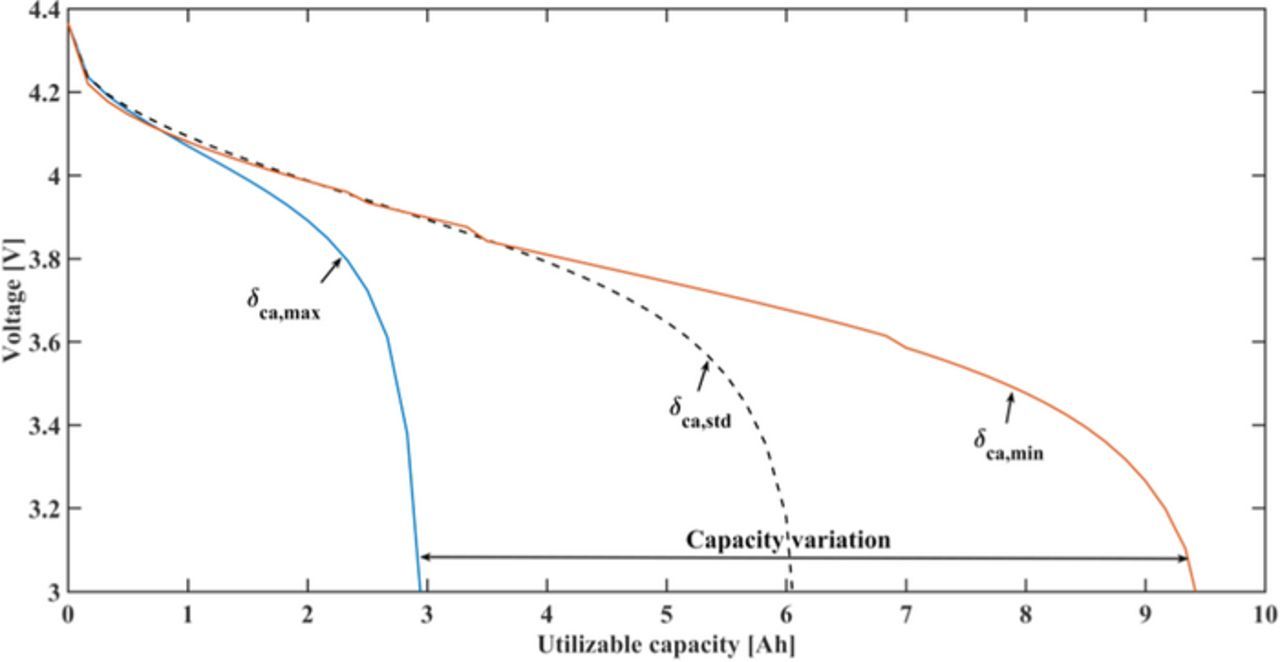
The global sensitivity can easily evaluate the sensitivities of performance to a group of cell parameters based on the variation ranges for specific outputs, in this section, the output is utilizable discharge capacity. The utilizable discharge capacity is defined as the discharge capacity when cell voltage reaches the cutoff value 3 V. As shown in Figure 3, for the given parameter set and parameter range in Table II, an increase of the cathode thickness to the upper bound leads to a decrease of utilizable discharge capacity, and a decrease of cathode thickness to the lower bound as used in this work results in an increase of capacity. Figure 3 illustrates a significant capacity variation by changing the cathode thickness. This is not only due to effects of the cathode thickness itself, but also due to the previously mentioned correlation of δan, Nlayer and δca. When the cathode thickness δca varies in the given range, the anode thickness δan and the number of active layers Nlayer also changes dramatically according to Equation 41 and 42 to maintain a proper balancing of the cell and the required cell capacity. The layer number Nlayer can change from 17 to 64. Since the pouch cell is made of stacked layers as shown in Figure 1, Nlayer strongly affects the distributed current on each current collector, thereby the current density on each current collector. Consequently, it affects the lithium transport and cell capacity. The strong negative effect of thick electrodes also needs to be attributed to strong transport limitation, as reported also in the reference.64 Understanding the sensitivities of parameters for cell performance is thus crucially important for optimization of cell design.
In Figure 4, we show the global sensitivities of all parameters for the utilizable capacity after galvanostatic discharge at 1C. Here, a subset of 10 sensitivities is significant, and the sensitivity of the cathode thickness is much larger than the others as it determines the design capacity of the cell. The specific capacity of the cathode material and the solid diffusion coefficients in both electrodes have the next strongest effects on the discharge capacity. This indicates that the discharge capacity at 1C is controlled by the solid diffusion processes, because the ability of lithium ion transport in solid phases determines the electrochemical performance according to the previous model development section. From these identified parameters, three cathode design parameters obtain higher sensitivities. The cathode thickness mainly determines the methodology of cell design, since the variation of cathode thickness also causes strong variation of layer number and anode thickness. To better evaluate the sensitivities of the other parameters, the cathode thickness is fixed to its standard value in the following studies because the cathode thickness has the highest sensitivity of all for its strong correlated effect on battery performance.
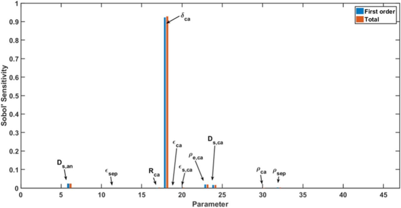
Figure 4. Global sensitivity of all 46 parameters for utilizable discharge capacity at 1C. First-order sensitivities represent the individual contribution of each parameter to the utilizable discharge capacity, and the total sensitivities including parameter interactions.
Next, after fixing the cathode thickness, all the other 45 parameters are divided into two groups for individual sensitivity studies. The first group represents the design parameters and includes 13 parameters as listed in the first part of Table II. They cover manufacturing factors and geometries, such as particle radius, porosity, current collector thickness, etc. In design parameters, we use Bruggeman coefficient b to represent tortuosity  .65,66 As the tortuosity of porous electrode can be described by Bruggeman relation, the Bruggeman coefficient can quantify tortuosity effect. The second group (32 parameters) contains the physical properties of the cell component materials, e.g., material densities, thermal conductivity, reaction kinetic parameters, etc. In Table IV, we illustrate the global sensitivities of the design parameters for the utilizable discharge capacity at 1C. Here, the current collector thickness and the cathode pore properties i.e., ca, bca and s, ca dominate the simulation outcome. An explanation of these sensitivities is that current collectors determine the local current density at the electro-active layers and the reaction kinetics. Furthermore, the ionic transport and the interface reactions in the electrodes are determined by the porosity and the pore structure. Thus, the cathode pore properties and its current collector thickness have more impact on the discharge capacity. In the investigated cell, the pore properties of the anode also show visible but weak effects on the discharge capacity, compared with the cathode pores. Therefore, on the utilizable discharge capacity at 1C of the investigated cell, the pore properties of both electrodes play an important role, and the cathode pores are more influential. A comparison of the first-order and total sensitivities of each design parameter reveals the apparent differences which indicates strong interactions with other parameters, especially of the current collector thickness and pore geometries.
Table IV. Global sensitivities of 13 design parameters for the utilizable discharge capacity at 1C after the cathode thickness δca and the physical property parameters are fixed. SCi denotes first-order Sobol' sensitivity of utilizable capacity. SCTi denotes total Sobol' sensitivity of utilizable capacity.
| Parameter | SCi | SCTi |
|---|---|---|
| Ran | 0.003 | 0.005 |
| an |
0 | 0.001 |
| s, an |
0.002 | 0.003 |
| ban | 0.003 | 0.007 |
| δcc, an | 0.117 | 0.129 |
| δsep | 0 | 0.003 |
| sep |
0.006 | 0.007 |
| bsep | 0.004 | 0.010 |
| Rca | 0 | 0.003 |
| ca |
0.271 | 0.401 |
| s, ca |
0.031 | 0.034 |
| bca | 0.139 | 0.269 |
| δcc, ca | 0.271 | 0.280 |
The parameter interactions are revealed in Figure 5. It shows that the Bruggeman coefficients bca, bsep, porosities ca, sep, an, and current collector thickness δca, δan have strong interactions with other parameters. The current collector thickness of the cathode has a strong interaction only with the current collector thickness of the anode. Due to the high thermal conductivities of the battery components, the heat transfer inside the battery proceeds via them mostly. This heat affects the temperature homogeneity inside the battery, thus it affects the local electrochemical performance on each electrode. The pore geometries of the cathode, anode, and separator are the main variables that affect the ionic transport in the electrodes together. According to Equations 4 and 5, the electrochemical performance is influenced by ionic transport in every cell domain. Therefore, the pore geometries in the cathode, anode, and separator interact via the discharge capacity. The cathode particle radius Rca also shows a clear interaction with the Bruggeman coefficient in the separator bsep. This is because both parameters strongly determine the overpotentials from solid lithium diffusion process and ionic transport in the electrolyte. As the total overpotential of the cell is related to discharge capacity, Rca and bsep have a strong interaction for utilizable discharge capacity. Similarly an interaction between Ran and bsep exists. The impact of interaction between Rca and bsep on utilizable discharge capacity is shown in Figure B1 in Appendix B.
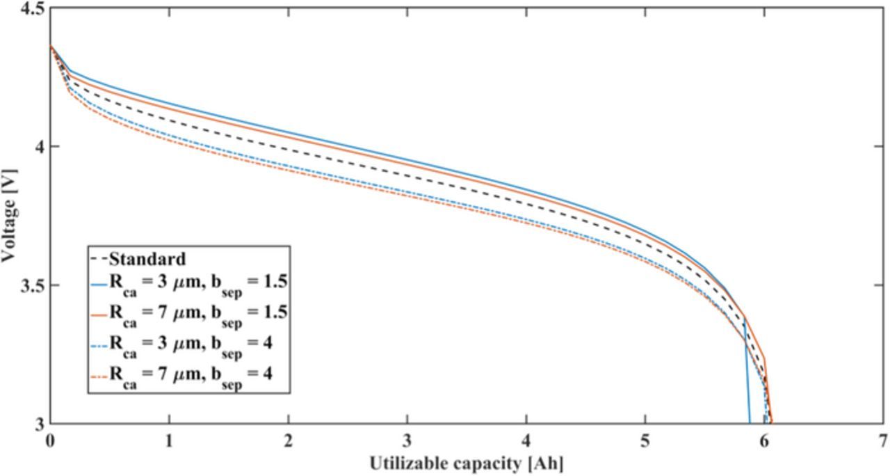
Figure B1. Capacity-voltage curves with varying cathode particle size Rca and Bruggeman coefficient in the separator bsep. Standard parameter value see in Table II.
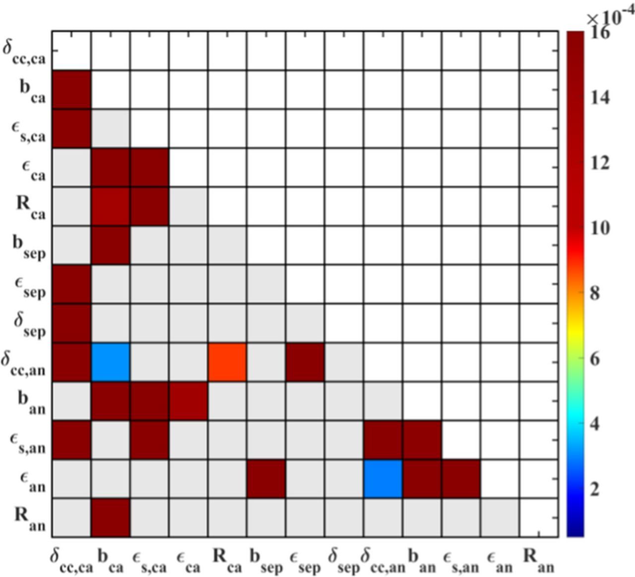
Figure 5. Second-order sensitivities of 13 design parameters for the utilizable discharge capacity, with the constant cathode thickness δca and physical property parameters. The gray elements show no interactions between the parameters.
Figure 6 demonstrates the parameter dependency of the physical properties, in turn. The utilized discharge capacity of the cell is mainly determined by the solid diffusion coefficients of both electrode particles and the specific capacity of the cathode material, with smaller interactions compared with the design parameter group. According to Equations 4 and 5, the solid diffusion process directly affects the electrochemical performance. Based on our assumed manufacturing process, the specific capacity of the cathode determines the electro-active layer numbers and thus determines the current density of each current collector. Therefore, among the parameters in the physical property group, these three parameters have a significant impact on the cell discharge capacity. In addition to the design parameters, the remaining parameters of the physical property group do not have a significant influence on the discharge capacity as shown in Figure 4. Thus, we do not show the calculation of the parameter interactions for the physical property parameters. It is interesting to observe that the discharge capacity at low C-rates is less sensitive to the thermal properties of the cell component materials. It means that the temperature does not evidently affect the discharge process at low C-rates. Thus, for the investigated cell, the discharge capacity at 1C is quite sensitive to the electrode material design, including the structure and the shape.
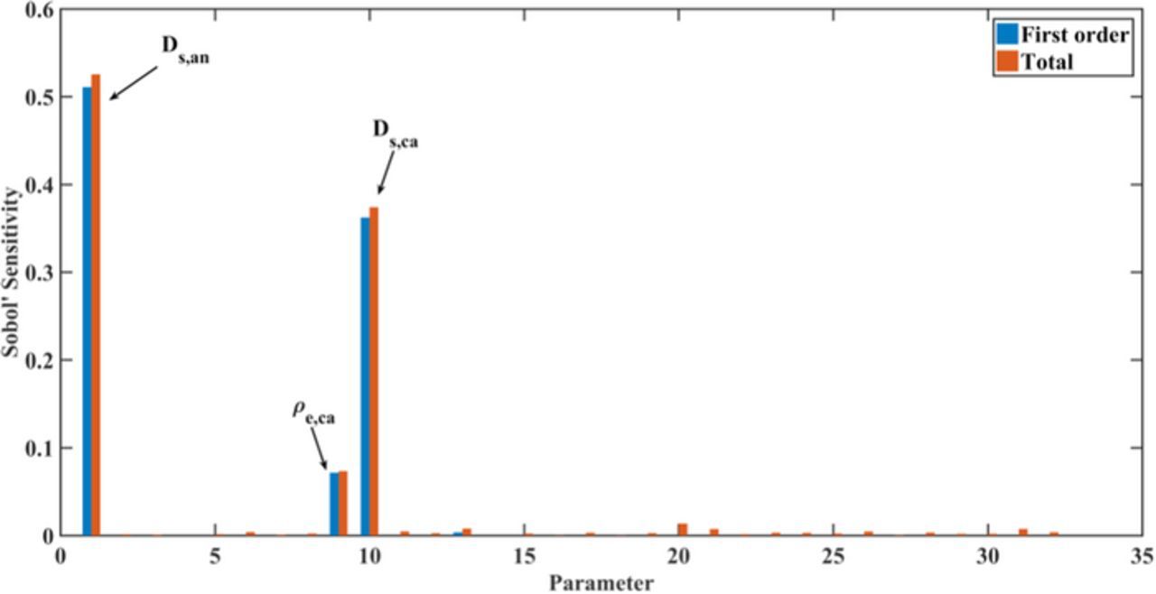
Figure 6. Global sensitivities of 32 physical property parameters for the utilizable discharge capacity at 1C after the cathode thickness δca and design parameters are fixed.
Maximum cell temperature
For a large-format pouch cell, the investigation of thermal behavior is also critical because the heat in larger cells may not be removed sufficiently fast, finally causing local overheating. Therefore, we consider the maximum cell temperature during operation as a second case for sensitivity analysis. It is a good candidate for safety management in large cells. The maximum temperature of the cell is located close to the tab in the center layer as shown in Figure 7. Based on temperature ranges in Figure 7, we can also conclude that the variation of cathode thickness has a strong impact on cell temperature evolution and variation.
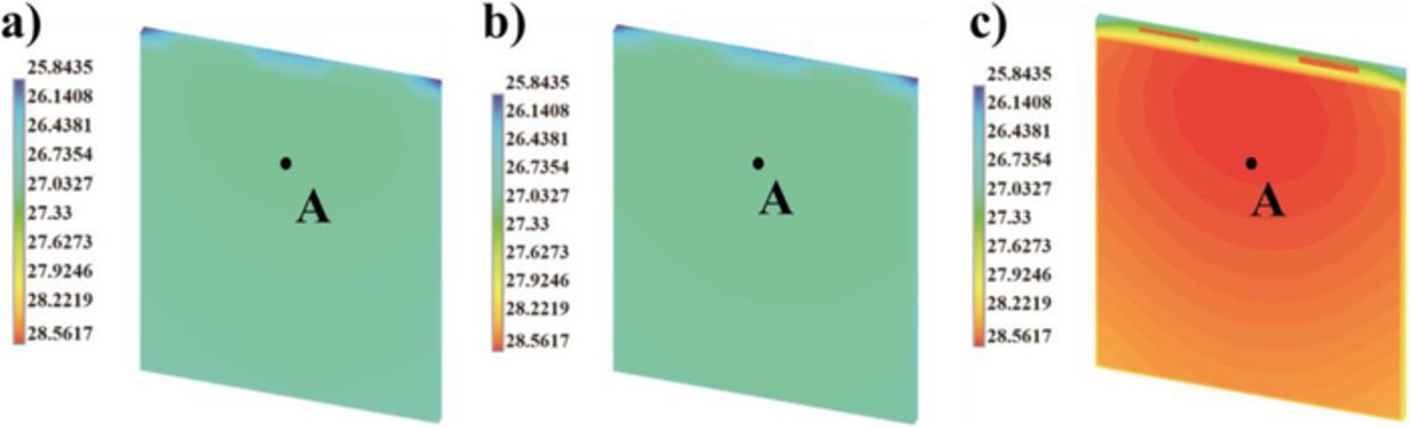
Figure 7. Temperature distribution [°C] on cross-section of the central layer at the end of 1C discharge, with varying cathode thickness, a) standard 60 μm; b) minimum 30 μm; c) maximum 100 μm. Point A is defined the evaluated point of maximum cell temperature.
We evaluate the maximum cell temperature on position A displayed in Figure 7, at the end of the 1C discharge followed by the proposed stepwise design. In Figure 8, we show the global sensitivity results for all 46 parameters for the maximum cell temperature at 1C discharge. Compared with the utilizable discharge capacity, more parameters have significant impacts on the maximum cell temperature. Cathode thickness and pore size strongly affect the maximum temperature of the analyzed cell. The difference between the first-order and total sensitivities indicates significant parameter interactions, due to the strong correlated effect of cathode thickness. The maximum cell temperature is also apparently influenced by the anode pore size, the particle size, the electric conductivities of active materials, and the electrolyte transport properties. Based on Equations 7 to 10, the ionic transport in the electrolyte, the electron conduction in electrodes, and interface reactions mainly contribute to the ohmic and reaction heat, respectively, during operation. These physical processes are affected by the electrodes and their pore structures, the electrolyte properties, and the electric properties of the electrodes. In contrast to the discharge capacity, more parameters evidently affect the thermal behavior of the cell. Physical property parameters still play a minor role in the thermal performance of the cell. Note that most of the sensitive parameters significantly interact, as shown in Figure 8. Therefore, it is necessary to evaluate parameter interactions in both groups as well.
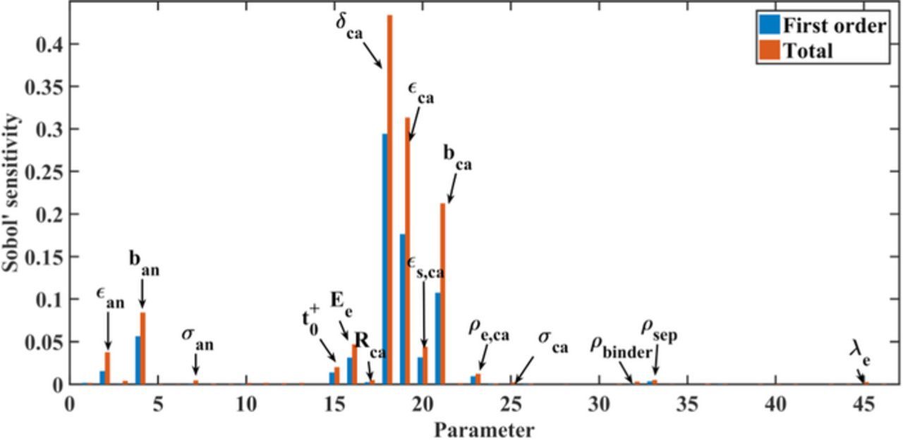
Figure 8. Global sensitivities of all 46 parameters for the maximum cell temperature at 1C discharge.
For a first step, for avoiding strongly correlated parameter and studying design parameter set, we fixed the physical property parameters and the cathode thickness and vary the design parameters exclusively. In Table VtA1tA2, we illustrate the global sensitivities of 13 design parameters for the maximum cell temperature at the 1C discharge. In contrast to the sensitivities for the discharge capacity, all 13 design parameters for the maximum cell temperature have visible total sensitivities, and the cathode pore structure and the particle size have the largest effects among them. It indicates that all design factors are involved in the thermal behavior of the cell individually or indirectly, and the cathode design factors dominate. The pore geometries and the particle radius in cathodes indicate that the generated heat of the battery mainly results from the ohmic and reaction heat during operation. When the first-order and total sensitivities are compared, there are significant parameter interactions for the maximum cell temperature.
Table V. Global sensitivities of 13 design parameters for the maximum cell temperature at 1C after the cathode thickness δca and physical property parameters are fixed. STi denotes first-order Sobol' sensitivity of the maximum cell temperature. STTi denotes total Sobol' sensitivity of the maximum cell temperature.
| Parameter | STi | STTi |
|---|---|---|
| Ran | 0.005 | 0.012 |
| an |
0 | 0.015 |
| s, an |
0.005 | 0.023 |
| ban | 0.0246 | 0.039 |
| δcc, an | 0 | 0.010 |
| δsep | 0 | 0.003 |
| sep |
0.006 | 0.014 |
| bsep | 0.011 | 0.024 |
| Rca | 0.333 | 0.346 |
| ca |
0.178 | 0.294 |
| s, ca |
0.250 | 0.279 |
| bca | 0.015 | 0.133 |
| δcc, ca | 0 | 0.020 |
Note that the cathode thickness has a strong correlation with the other parameters regarding capacity sensitivities; see Figure 4 and Figure 9. This strong correlation might result in different sensitivity measures, when we divide the model parameters into two groups and assume a fixed value for cathode thickness. We, therefore, used the expected value of the cathode thickness to provide a representative sensitivity analysis of the individual group of the design parameters. A better understanding of the effect of the design parameters, in turn, is mandatory for an effective cell design and is discussed in more detail below.
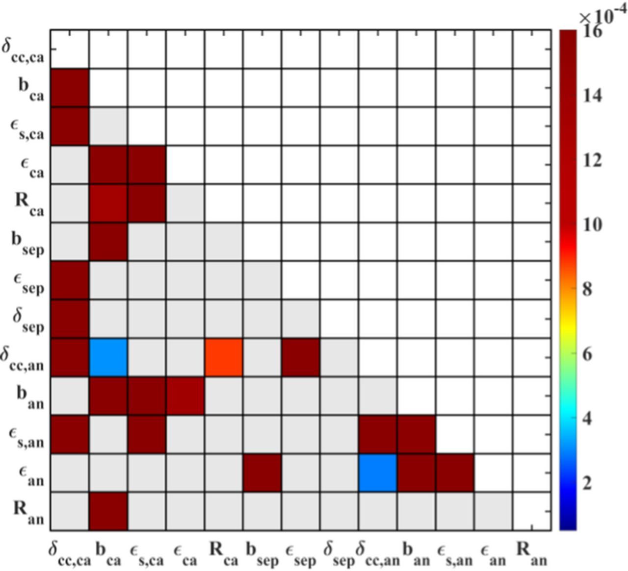
Figure 9. Second-order sensitivities of 13 design parameters for the maximum cell temperature at 1C discharge with the constant δca and physical property parameters. The gray elements show no interactions between the parameters.
The sensitivity matrix in Figure 9 reveals the parameter interactions for the maximum cell temperature. It is evident that there are more interacting parameters compared with the discharge capacity output in Figure 5. The porosities and the Bruggeman coefficients determine the pore structure and the pore volume. As mentioned earlier, at the electrode level, the heat generation is determined by the ionic transport and the electrode–electrolyte interfacial reactions. The reason is that the pore size and the structure determine the lithium ion transport in the solid and solution phases, and the electrode particle size influences the specific area and the reaction kinetics at the interfaces. The combined action finally affects the heat generation of the cell during discharge. Moreover, the thickness of the current collectors also interacts with the pore size and the electrode microstructure. This results from the current density and the heat transport through the current collector. As the current collectors distribute and collect the current to the solid and solution phases, the thickness of the two current collectors influences local heat generation and heat transfer, and this directly affects the maximum cell temperature.
At the cell level, it is interesting to see that the pore structure of the anode interacts with that of the cathode in Figure 9. It is because the pore geometries of both electrodes determine the solid volume of the whole battery, and thus, the number of electro-active layers and the heat conductivity of the battery, based on a fixed nominal capacity of the cell. If the pores are bigger and have more space, the total number of layers should be larger, and this results in a worse heat transfer from the inside to the outside, and it finally determines the maximum temperature of the cell.
Unlike the design parameters, significant sensitivities of the physical property group concentrate on only three parameters, as shown in Figure 10. The maximum cell temperature is most sensitive to the solid diffusion coefficient in the cathode particles. It indicates that the overpotential from the solid diffusion process in the cathode mainly contributes to the heat generation of the cell according to Equations 7 to 10. The specific capacity of the cathode material shows a visible but smaller sensitivity. This indicates that specific capacity of cathode material can also affect the accumulation of heat in the cell.
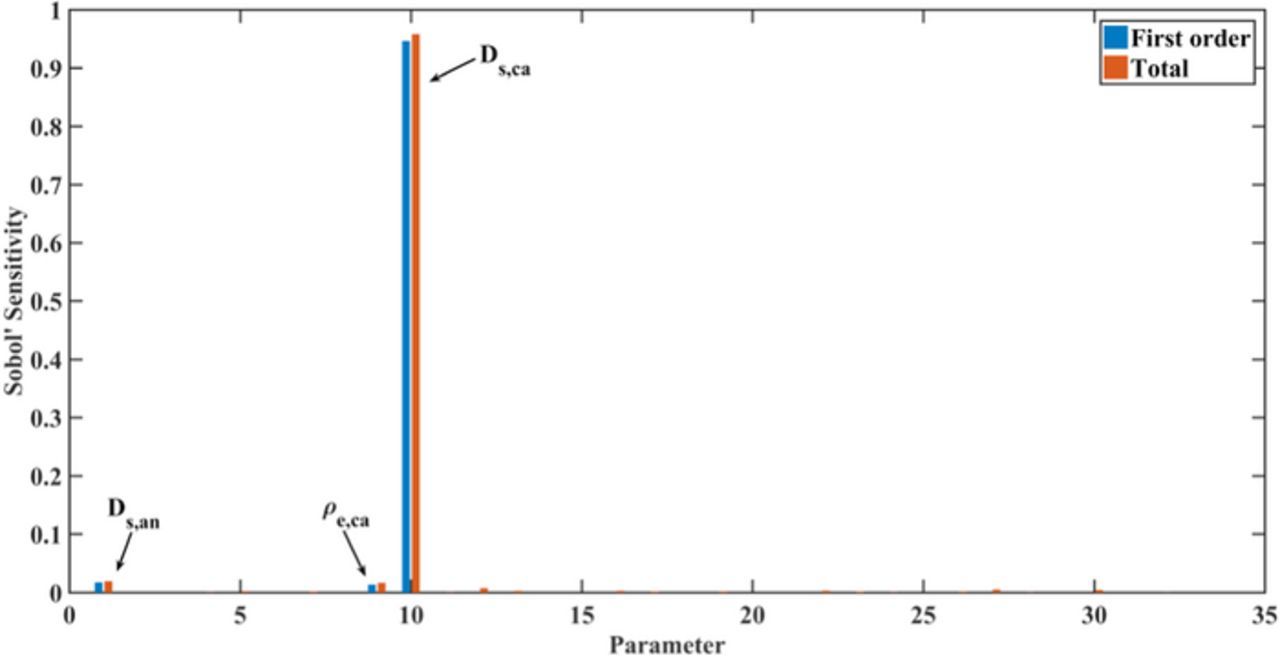
Figure 10. Global sensitivity of the physical property parameters for the maximum cell temperature at the end of the 1C discharge, with the constant cathode thickness δca and design parameters.
Conclusions
Perspectives
GSA reliably works for assigning confidence in model prediction and investigation of less know parameters that result in large uncertainties with small parametric deviations in highly non-linear systems.23 In non-linear Li-ion battery systems, it includes many uncertain parameters, such as electrode particle sizes, porosity, electrode structures and thermodynamics. In the case of complex, non-linear systems with large amount of parameters, GSA can effectively and efficiently quantify:
- (1)the relationship between parameters and objective outputs, for example battery performance,
- (2)parameter uncertainties for more reliable and accurate model predictions,
- (3)the parameter identifiability for simplification of complex model with high computational cost.
With these functions, more advanced models for large-format Li-ion batteries can be developed and improved by effectively identifying relevant uncertain parameters, thereby investigating and predicting detailed physical processes such as local temperature and discharge capacity, etc. In engineering perspectives, it will contribute much to design and optimization of different lithium-ion battery systems, and development of efficient on-line monitoring models for fast prediction and estimation of practical battery systems, for example, electric vehicles, large-format consumer electronic cells, battery management systems, etc.
Conclusion
A global sensitivity analysis of a 3D multiphysics model for a Li-ion cell was performed to analyze impacts of 46 parameters on cell performances including discharge capacity and temperature variation. For this, an efficient PCE method was implemented with a stepwise procedure. To overcome the difficulties of large computational costs due to the number of parameters, a sparsity-based and highly efficient version of PCE was applied. The number of random cases was drastically decreased, and the computational efficiency was improved. In this vein, 46 parameters of the 3D multiphysics model were efficiently identified and investigated in two studies, namely sensitivity to thermal performance by analyzing the maximum local cell temperature and sensitivity to electrochemical performance by analyzing the utilizable discharge capacity at 1C. Through the stepwise design approach, the cathode thickness was identified as the most sensitive parameter for the discharge capacity and the maximum cell temperature. Moreover, it was found that the discharge capacity and the maximum cell temperature at 1C were sensitive to nine design parameters, including the electrode particle sizes and the pore geometries of the investigated cell, and the parameters strongly interact with each other. For the discharge capacity, the cathode design parameters play an important role. The design parameters of all cell components are visibly sensitive to the maximum cell temperature as well. Within the physical property cluster, only the solid diffusion coefficient of the electrode particles and the specific capacity of the cathode material were sensitive to the utilizable discharge capacity. It shows that the utilizable capacity is related to electrode geometries. In contrast, the thermal behavior of the cell is affected not only by the electrode geometry but also by the cell geometry and the manufacturing process, which determine the thermal management of the battery.
To sum up, a global sensitivity study using the Sobol' indexes with a PCE approach is successfully and efficiently used for a 3D multiphysics model of a large-format Li-ion battery. This work also inspires future research. One aspect is the investigation of the performance of other efficient approaches for constructing CPU-friendly surrogate models, e.g., low rank approximation concepts. The other aspect is effective improvement in the efficiency of the cell design and battery testing process, i.e., only to concentrate varying highly sensitive parameters for cell performances, it is easy to optimize a well-managed cell design for higher energy/power densities and evaluate hot spots inside the cell to reduce safety risks. Moreover, battery tests can be more effectively designed based on monitoring outputs and highly sensitive parameters.
List of Symbols
| A | Cross section area of electrode plate, m2 |
| A+, A− | Area of current collector tabs, m2 |
| ai | Specific area of electrode particles, m2/m3 |
| bi | Bruggeman coefficient of cell components, 1 |
| CP | Specific heat capacity, J/kg K |
| ce | Salt concentration in electrolyte, mol/m3 |
| cs, max, i | Maximum lithium concentration in electrode particles, mol/m3 |
| cs, surf, i | Surface lithium concentration in electrode particles, mol/m3 |
| f | Mean molar activity coefficient of electrolyte |
| F | Faraday constant, 96485 C/mol |
| I | Applied current, A |
| Istack | Applied current on each current collector, A |
| Inode | Local current on nodes of electro-active layer, A |
| ix | Current density in solid phases, A/m2 |
| i0, i | Exchange current density, A/m2 |
| jx, i | Pore-wall flux at the electrode-electrolyte interface, mol/m2 |
 |
Lumped average pore-wall flux, mol/m2 |
| k | Thermal conductivity, W/m K |
| k0, i | Lithium intercalation reaction kinetics, m2.5/mol0.5 s |
| L | Total thickness of one electrochemical active layer, m |
| Nelem | The number of electro-active nodes |
| p | The maximum order of multivariate polynomials |
 |
Volumetric heat source, W/m3 |
| Ri | Electrode particle radius, m |
| Si | First order sensitivity of parameter i |
 |
Total sensitivity of parameter i |
| T | Temperature, K |
| t | Time, s |
| Ui | Open circuit potential, V |
Greek
| α | Charge transfer coefficient |
| αk | Coefficient for the kth multivariate polynomial |
| βh | Convective heat exchange coefficient, W/K m2 |
| δi | Thickness of electrodes or separator, m |
| b, i |
Volume fraction of binder |
| i |
Porosity |
| s, i |
Volume fraction of electrode solid matrix |
| ηi | Overpotential, V |
| κi | Ionic conductivity, S/m |
| λn, λN, λN + 1 | Eigenvalue |
| σi, σj | Electric conductivity, S/m |
| ρ | Material density, kg/m3 |
| ρe, i | Specific capacity of electrode material, Ah/kg |
| ϕkii(Xi) | Univariate polynomial with the order of ki for parameter i |
| Φe | Potential in electrolyte, V |
| Φs, i | Potential in solid phase, V |
| Φj | Electric potential on current collectors on cell level, V |
| Ψk(X) | The kth multivariate polynomial |
Subscripts
| amb | Ambient |
| an | Anode |
| ca | Cathode |
| e | Electrolyte |
| eff | Effective |
| i | Indice of electrode |
| j | Indice of current collector |
| np | Number of the parameters |
| P | Constant pressure |
| r | Reaction |
| S | Entropy |
| s | Solid |
| sep | Separator |
| x | 1D Cartesian coordinate x on electrode level |
| Ω | ohmic loss |
| + | Cathode current collector |
| − | Anode current collector |
Acknowledgment
The authors thank MWK Niedersachsen for funding with the Promotionsprogramm "μ-Props" and appreciate Guofang Huang's contributions of case simulations in this article.
ORCID
Nan Lin 0000-0003-0083-6804
Ulrike Krewer 0000-0002-5984-5935
Appendix A:: Further model parameters
Open circuit potential (OCP) is calculated by a function of θ as follows
For cathode (fitted by the data of Lenze et al.9):
![Equation ([A1])](https://content.cld.iop.org/journals/1945-7111/165/7/A1169/revision1/d0041.gif)
For anode:15
![Equation ([A2])](https://content.cld.iop.org/journals/1945-7111/165/7/A1169/revision1/d0042.gif)
![Equation ([A3])](https://content.cld.iop.org/journals/1945-7111/165/7/A1169/revision1/d0043.gif)
where  .
.
Ionic conductivity:15
![Equation ([A4])](https://content.cld.iop.org/journals/1945-7111/165/7/A1169/revision1/d0044.gif)
: Appendix B
Figure B1 shows that the capacity range based on the range of cathode particle size Rca is also related to the value of Bruggeman coefficient in the separator bsep. With a smaller bsep, the capacity variation range is larger, and the minimum and maximum values of utilizable discharge capacity are also different from another case with a larger bsep. It indicates that bsep and Rca have an interacted effect on the utilizable discharge capacity.