Thermal Design for the Pouch-Type Large-Format Lithium-Ion Batteries: I. Thermo-Electrical Modeling and Origins of Temperature Non-Uniformity

Bin Wu; Zhe Li; Jianbo Zhang

doi:10.1149/2.0831501jes

Lithium-ion batteries have been widely used in pure and hybrid electric vehicles due to their high energy density and long cycle life. Among the three major configurations for the power batteries, the pouch-type has attracted much attention of automotive manufacturers.^1,2 Nissan LEAF is equipped with a battery pack consisting of 192 pouch cells. The capacity of each cell is 33.1 Ah,¹ 10 times larger than that of the conventional 18650 cell. Similarly, GM VOLT uses 288 pouch cells. Each cell has a capacity of 45 Ah.² The much increased capacity of the large-format cell generates new problems that have not been observed or researched previously. In particular, a large temperature variation inside a cell develops, causing accelerated degradation, even triggering thermal runaway from hot spots.³

Modeling and simulation is an important method to address these new problems and to provide insights for cell design optimization. Battery models applicable at different length scales, ranging from the primary particles of active material to the battery pack, have been developed. A comprehensive review of the battery modeling can be found in Ref. 4.

Temperature is one of the key elements in the battery modeling. In a small cell, a lumped thermal model neglecting temperature distribution is fairly adequate. As the cell size increases, however, the spatial non-uniformity of the temperature grows rapidly to adversely affect the performance, life and even safety of the cell. Therefore, the temperature distribution must be evaluated together with the electrical behavior for the large-format cell. To such end, a thermo-electrical model is essential.

Kim et al.^5–10 proposed a computationally efficient model to predict the thermal and electrical behaviors for the pouch cell. In the electrical sub-model, the electrical potentials of the current collector are calculated using the Ohm's law, and the current density traversing the separator is assumed to be a function of the potential difference between the positive and negative electrodes. In the thermal sub-model, the heat generation rate in the battery core is calculated using the current density from the electrical sub-model. The model proposed by Kim is generic and forms a basis from which a number of variations developed. Guo et al.¹¹ used a pseudo two-dimensional electrochemical model to calculate the local heat generation rate. Gerver et al.¹² introduced a non-linear resistance to account for the relationship between the transverse current and the potential difference.

In terms of the model parameters, model validation, and the interpretation of the observed and simulated thermal features, there still exist several shortcomings in the thermal modeling of the cell in the literature:

(1)
Most reports cited thermal parameters, i.e. thermal conductivities and specific heat capacity, from the literature, sometimes ignoring the difference in battery composition or even structure, leaving the accuracy of thermal parameters in doubt. Meanwhile, the impact of the accuracy of thermal parameters on simulation results has not been evaluated either.
(2)
Kim et al.¹⁰ have suggested that the heat generated by the contact resistance between the tab and the leading cable has significant influence on the battery temperature distribution. In their work, they adjusted the value of contact resistance to fit the simulated temperatures to the measured results. The fitting method is not convincing because the agreement between the simulation and experiment results depends on the accuracy of many other parameters. However, few publications reported measured the value of the contact resistance.
(3)
Some thermal models are validated using the temperature measured from only one thermocouple attached on the battery surface. This single-point temperature validation may be acceptable for the small battery, but it is far from adequate for the large-format battery exhibiting severe temperature non-uniformity during cycling.
(4)
The origins of the temperature non-uniformity are still unclear. Possible causes to the temperature non-uniformity include the non-uniformity of the heat generation rate, poor thermal conductivity of the battery and the heating effect of the tab. However, the relative importance of those factors has not been discussed sufficiently.

Using the governing equations initially introduced in the work of Kim et al.,^5–10 this work proposes a multi-dimensional thermo-electrical model with reliable parameter inputs and rigorous experimental validation. This paper makes progress in the following respects. First, key parameters in the model, including the thermal parameters of the battery and the contact resistance between the tab and the cable, are estimated from carefully designed experiments. Second, the simulated temperatures are validated using multiple thermocouples to ensure the accuracy of the model. Third, sensitivity analysis for thermal parameters is conducted to assess the relative importance of different thermal parameters. Fourth, the origins of the temperature non-uniformity are discussed. It is found that the most important factor is the heating effect of the tab, rather than the non-uniformity of the heat generation rate in the battery core.

Modeling

A 25 Ah pouch-type lithium-ion battery was studied in this work. The specifications of the battery are listed in Table I.

Table I. Specifications of the battery.

Cell specification	Value
Capacity (1/3C, 25°C)	25 Ah
Nominal voltage	3.8 V
Cathode	LiMn_xCo_yNi_zO₂ and LiMn₂O₄
Anode	Graphite
EODV (end of discharge voltage)	3 V
EOCV(end of charge voltage)	4.2 V
Number of electrode pairs	18
Thickness	7.2 mm
Highest discharge rate	3 C for 30 s
Highest charge rate	1.5 C for 30 min

Model development

The battery consists of 18 pairs of electrodes. A representative cell consisting of one positive electrode and one negative electrode is chosen to model the electrical behavior of the battery, as shown in Fig. 1. The current flow in the current collector is assumed to be two-dimensional due to the small thickness in Z direction (∼10 μm) compared to the other dimensions in X and Y directions (∼20 cm).^5–10 The transverse current through the separator is assumed to be perpendicular to the current collectors as the distance between the electrodes is very small.^5–10

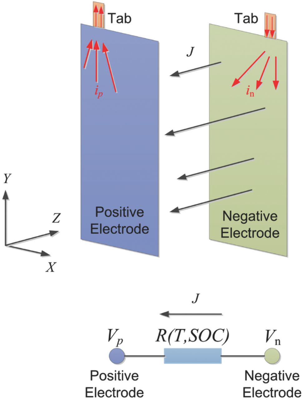
**Figure 1.** Schematic of the electrical model.

Accordingly, the governing equation for the charge balance in the current collector is^5–10

where σ_j is the electrical conductivity of the current collector (S m⁻¹), Φ_j the potential distribution on the of the current collector (V), J the transverse current density (A m⁻²), n the unit inward normal vector, δ_j the thickness of the current collector (m). The subscript j corresponds to the positive or negative electrode.

The boundary condition at the interface between the positive electrode and positive tab is

Where I_cell is the discharge current of one single cell (A), L is the width of the tab (m).

The boundary condition at the interface between the negative electrode and negative tab is

Other boundary conditions are assumed to be electrical insulated:

The transverse current density is defined as:

Where U_OC is the open-circuit potential of the cell (V) and varies with temperature and state of charge (SOC) over the electrode domain, R is the overpotential resistance per unit area (Ω m²). U_OC and R were determined experimentally.

The energy conservation equation for the battery core is:

where ρ is the density (kg m⁻³), C_p the specific heat capacity (J kg⁻¹ K⁻¹), T the temperature (K), k_in the in-plane thermal conductivity (W m⁻¹ K⁻¹), k_th the through-plane thermal conductivity (W m⁻¹ K⁻¹) and Q the heat generation rate (W m⁻³). The values of k_in, k_th and C_p are determined in Parameter determination section.

According to the Bernardi heat generation model, the total heat generation rate of the battery core is:¹³

where q_rev is the reversible heat generation rate (W m⁻³), q_irev the irreversible heat generation rate (W m⁻³), q_CCj the Joule heat generation rate of the current collector (W m⁻³) and d_PE, d_S, d_NE correspond to the thickness of positive electrode, separator and negative electrode (m), respectively.

In the tab, the Joule heat generation rate is the sole heat source:

where I_tab is the current flowing through the tab (A), A_tab the cross-section area of the tab (m²), σ_{tab, j} the electrical conductivity of the tab (S m⁻¹) and σ_{c, j} the equivalent conductivity of the electrical contact between the battery tab and the leading wire (S m⁻¹). The determination of σ_{c, j} will be introduced in Parameter determination section.

The convective boundary condition for the battery surface is written as:

where q_conv is the heat flux transferred to the air owing to the heat convection (W m⁻²), h the convection heat transfer coefficient (W m⁻² K⁻¹) and T_amb the ambient temperature (K). The value of h is determined in Parameter determination section.

Fig. 2 depicts the coupling method between the two models. First, the two-dimensional electrical model based on Eqs. 1∼5 is used to calculate the distribution of current density and electrical potentials. Then, the results from the electrical model are used to calculate the heat generation rate in the battery core, as described in Eqs. 7∼10. Afterwards, the heat generation rate is served as a source term in the three-dimensional thermal model to calculate the temperature distribution. Last, the temperature is transferred to the electrical model to determine the temperature-dependent variables, such as the resistance.

**Figure 2.** The coupling method between the 2D electrical model and 3D thermal model.

In the two-dimensional electrical model, the temperature is set as the average temperature along the Z axis at the corresponding location of the three-dimensional thermal model:

In the three-dimensional thermal model, the heat generation rate is assumed to be uniform along the Z axis, which is equal to the result at the corresponding location in the two-dimensional electrical model:

Parameter determination

Thermal conductivities and specific heat capacity

Most reports cited thermal conductivities and specific heat capacity in Eq. 6 from the literature, sometimes even ignoring the differences between different batteries, which leave the accuracy of thermal simulation doubtful. The authors have developed a joint experimental and computational method to estimate the thermal parameters of the pouch-type lithium ion battery.¹⁴ The general procedure of the method is reviewed in this paper and the details of the method can be found in Ref. 14.

The experimental setup is shown in Fig. 3. A thin circular ceramic heater was sandwiched between two identical 25 Ah batteries from the same manufacturer. The two batteries were covered from upside and downside with polyfoam for thermal insulation. Eight thermocouples, A1∼A4 and B1∼B4 were placed at strategically-chosen locations between the battery and the polyfoam.

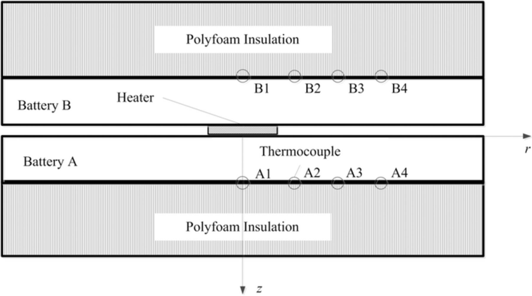
**Figure 3.** Schematic diagram of the experiment setup for the measurement of thermal parameters.

In the experiment, the batteries were heated by the circular heater in constant power mode, and the temperature responses were recorded with the eight thermocouples. This thermal system was modeled using a two-dimensional axially-symmetric model containing specific heat capacity and anisotropic thermal conductivities. The axis-symmetric assumption of the thermal system is utilized to reduce the computational cost of the parameter estimation process, and the assumption is verified with the results of the infrared thermal imaging and thermocouples.¹⁴ Using optimization technique, these thermal parameters were adjusted step by step till the difference between the simulated and the experimental temperature responses at the corresponding locations reaches a minimum.

The estimated specific heat capacity is 1243 J kg⁻¹ K⁻¹, the in-plane thermal conductivity is 21 W m⁻¹ K⁻¹ and the through-plane thermal conductivity is 0.48 W m⁻¹ K⁻¹. The estimated error of the specific heat capacity was about 10%, which was validated with the accelerating rate calorimeter (ARC) and the heat flow calorimeter (HFC).

Electrical contact resistance and convection heat transfer coefficient

The electrical contact resistance between the battery tab and the leading cable is generally ignored in the literature with the exception of Ref. 10. In Ref. 10, the contact resistance was an adjustable variable to provide the best agreement between the simulated and the measured temperatures. The adjusted contact resistance was a comparable value with the tab resistance, which indicates the heating effect of the contact resistance cannot be ignored. In this work, a new method is developed to simultaneously estimate the electrical contact resistance and convection heat transfer coefficient of the tab.

Fig. 4 depicts the schematic of this method. A separate tab was connected to two cables using nuts and bolts. The tab used in this experiment is the same with the real battery tab, and the experiment setup resembles the real current flowing direction. The connection method between the tab and cable is similar to the battery discharge testing, thus the estimated contact resistance from this experiment is applicable for the battery. The tab was electrified with high current, and the temperature increase due to the electrical heating was recorded with a thermocouple attached on the tab surface.

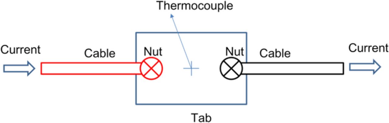
**Figure 4.** Schematic of the experiment to estimate the electrical contact resistance.

Owing to its high thermal conductivity and the small thickness, the tab is assumed to exhibit uniform temperature distribution during the experiment. Based on the energy conservation equation, the temperature of the tab T_t can be written as:

where ρ_t is the tab density (kg m⁻³), C_pt the specific heat capacity of the tab (J kg⁻¹ K⁻¹), T_t the temperature of the tab (K), q_t the heat generation rate owing to the ohmic and contact resistance (W m⁻³), h_t the convection heat transfer coefficient on the surfaces of the tab (W m⁻² K⁻¹), d_t the thickness of the tab, T₀ the environmental temperature (K).

The heat generation rate is:

where I is the electrified current of the tab (A), L_t the width of the tab (m), σ_t the electrical conductivity of the tab material (S m⁻¹) and σ_ct the equivalent conductivity of the electrical contact between the tab and the leading cable (S m⁻¹). There are two cables connecting the tab in the experiment, thus the number "2" appears in Eq. 17.

The initial temperature is defined as

The analytical solution for the Eqs. 16∼18 is

The contact resistance and the convection heat transfer coefficient are the adjustable parameters to provide the best fit of the calculated temperature to the experimental results. To check the feasibility of the method, two levels of current (37.5 A and 50 A) were adopted. As the convection heat transfer coefficient and the equivalent conductivity are independent on the current, the estimated results for different current levels should be the same.

Fig. 5 shows the experimental and fitted temperature curves of the positive tab and negative tab.

**Figure 5.** Comparison of experimental and fitted temperature curves of the tab: (a) Positive tab (b) Negative tab.

The estimated results listed in Table II show that the equivalent conductivity σ_ct has a comparable magnitude to the electrical conductivity σ. The narrow confidence intervals and similar results under different current levels validate the credibility of the method.

Table II. The estimated equivalent conductivity and heat convection coefficient.

	Current I (A)	Equivalent conductivity σ_c(S m⁻¹)	Heat convection coefficient h (W m⁻² K⁻¹)
Positive tab	37.5	79.4 × 10⁶	2.8
		[79.6 × 10⁶, 83.6 × 10⁶]^*	[2.8, 2.9]
	50	92.4 × 10⁶	2.9
		[87.4 × 10⁶, 98.0 × 10⁶]	[2.8, 2.9]
Negative tab	37.5	80.4 × 10⁶	2.9
		[79.0 × 10⁶, 81.6 × 10⁶]	[2.9, 3.0]
	50	72.0 × 10⁶	3.4
		[71.0 × 10⁶, 73.0 × 10⁶]	[3.3, 3.4]

*[,] corresponds to the 95% confidence intervals.

Open-circuit potential and entropy coefficient

The open-circuit potential curve was measured at 11 different SOCs, from 0.0 to 1.0 and in a step length of 0.1. The equilibrium state is defined when the voltage change rate is less than 0.1 mV/30 min. The measured results are shown in Fig. 6.

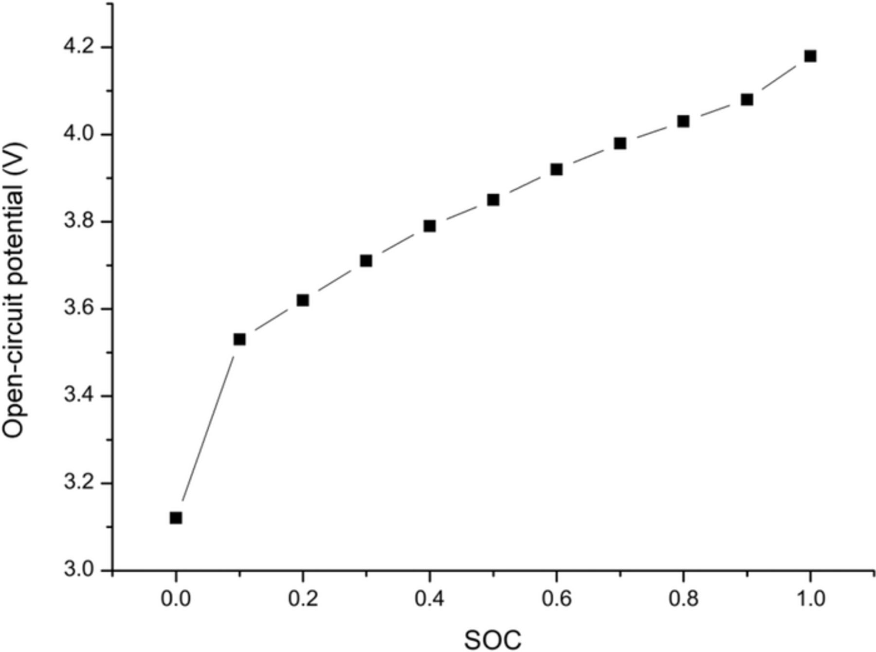
**Figure 6.** Open-circuit potential at different states of charge.

To obtain the entropy coefficient for the calculation of reversible heat generation rate, the equilibrium potentials U_OC at all evaluated SOCs were measured at a series of temperatures. The entropy coefficients were attained by calculating the slope of the fitted 'temperature-potential' line. With the SOC of the cell adjusted in a step length of 0.1 each time, the entropy coefficients at each different SOC were obtained. Fig. 7 shows the measured entropy coefficients with respect to SOC.

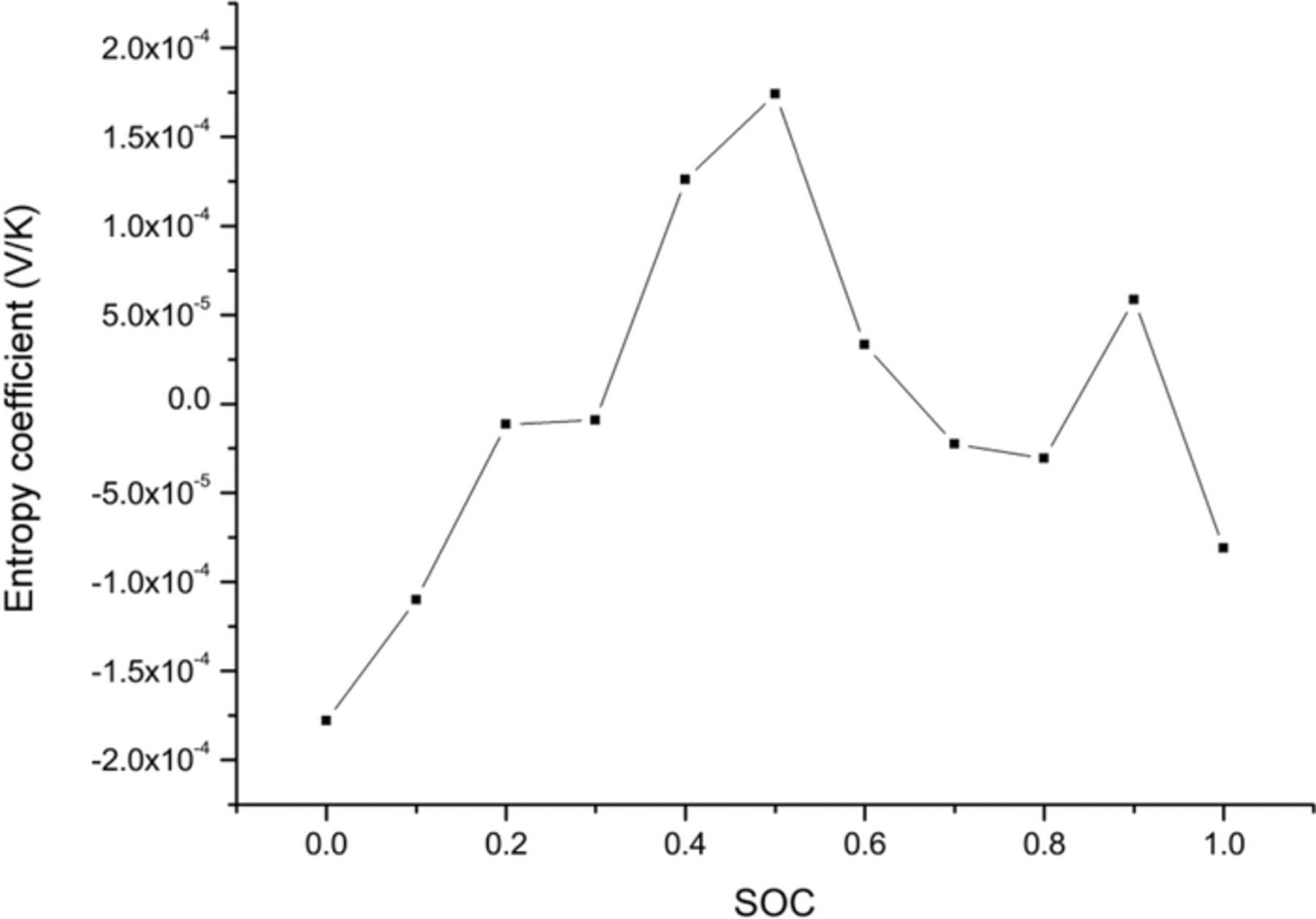
**Figure 7.** Entropy coefficient at different states of charge.

Overpotential resistance

The overpotential resistance is used to calculate the current density and irreversible heat generation rate, as noted in Eq. 5 and Eq. 9. Various methods have been proposed and utilized to estimate the overpotential resistance of the battery in the literature.¹⁵ Zhang et al.¹⁶ measured the overpotential resistance of a 25 Ah battery using three methods, the intermittent current method, the V–I characteristics method and a newly developed energy method. By comparing the calculated heat generation rates with the heat generation rate measured in an ARC, Zhang et al. found that the intermittent current method with an appropriate interval (60 s) achieves the highest accuracy.

In this work, the intermittent current method with an interval of 60 s was used to measure the overpotential resistance at different states of charge and temperatures in this work. The schematic diagram of the method is shown in Fig. 8. During the test, the battery was charged at 0.5 C for 2 min, rested for 8 min and then was discharged at 0.5 C for 2 min (for SOC = 100%, the battery was discharged first). The test was repeated at three temperatures (25°C, 30°C and 35°C) and 11 SOCs (from 100% to 0 with the step of 10%).

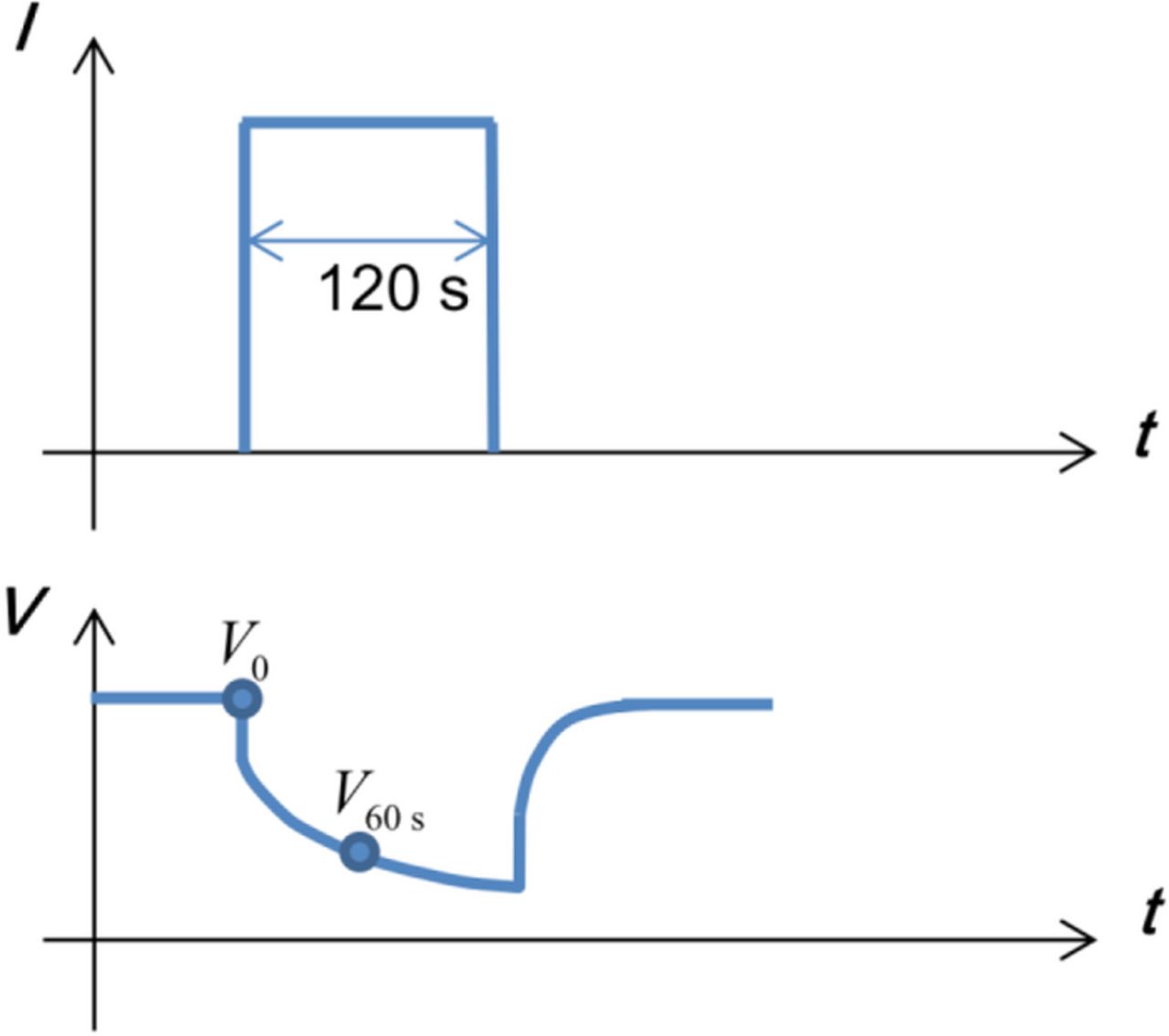
**Figure 8.** Schematic diagram of the intermittent current method.

The equivalent intermittent current resistance can be written as:

where V_60 s is the voltage after 60 s charge/discharge (V), V₀ is the voltage before the current pulse (V) and I is the pulse current (A). As the pulse current is 0.5 C, the SOC change owing to the 60 s pulse discharge/charge is 0.8%, which is a negligible SOC error for the thermal simulation.

The measurement results in Fig. 9 shows that the resistance dramatically increases at the low SOC range (10%∼0%) and slightly decreases as the temperature increases from 25°C to 35°C. R_IC (Ω) in Fig. 9 was converted to the overpotential resistance per unit area R (Ω m²) to be applicable in Eq. 5 and Eq. 9.

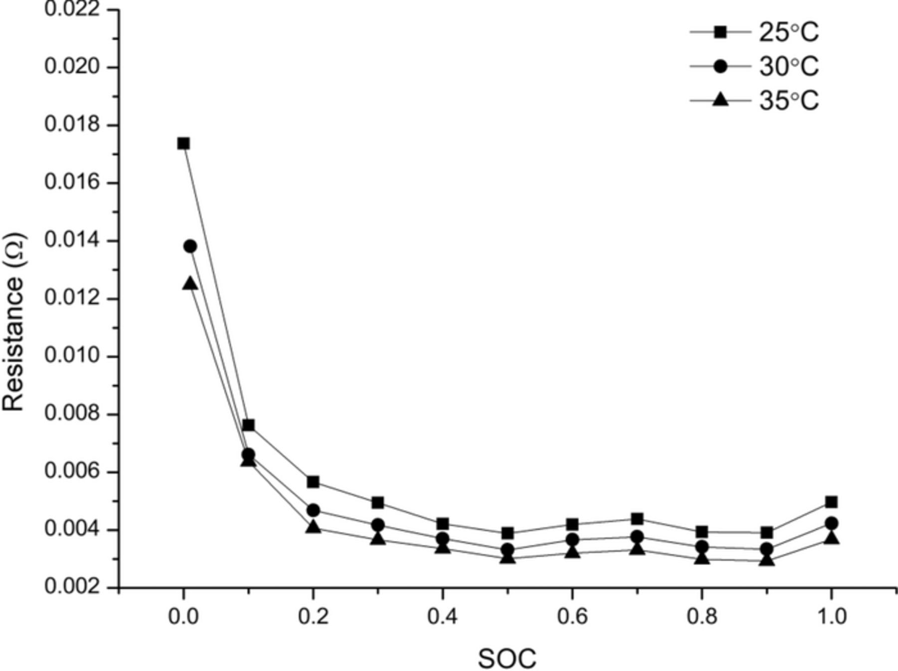
**Figure 9.** Overpotential resistance at different temperatures and states of charge.

The input parameters for model are summarized in Table III. The convection heat transfer coefficients for the battery core and the tabs, and the equivalent electrical conductivity between the tab and cables were slightly adjusted to achieve the best agreement between the simulation and the experimental results.

Table III. Input parameters for the model.

Current collector
	Positive		Negative
Current collector thickness δ_j (μm)	20		14
Current collector electric conductivity σ_j(S/m)	37.8 × 10⁶		59.6 × 10⁶
Tab width L (mm)	50
Electrode height (mm)	205
Electrode width (mm)	166
Electrode
	Positive	Separator	Negative
Thickness (μm)	20	30	14
Thermal conductivity k_in (W m⁻¹ K⁻¹)		21
Thermal conductivity k_th (W m⁻¹ K⁻¹)		0.48
Heat capacity C_p (J kg⁻¹ K⁻¹)		1243
Density ρ(kg m⁻³)		2300
Convection heat transfer coefficient h (W m⁻² K⁻¹)		4
Battery thickness (mm)		7.2
Tab
	Positive		Negative
Thickness (mm)	0.3		0.3
Width (mm)	50		50
Height (mm)	50		50
Thermal conductivity (W m⁻¹ K⁻¹)	237		401
Heat capacity (J kg⁻¹ K⁻¹)	900		385
Density (kg m⁻³)	2700		8700
Electrical conductivity (S m⁻¹)	37.8 × 10⁶		59.6 × 10⁶
Equivalent contact conductivity (S m⁻¹)	70 × 10⁶		80 × 10⁶
Convection heat transfer coefficient h (W m⁻² K⁻¹)	4

Results and Discussion

Results and validation

The finite element model described in the previous section was solved using a commercial software package, COMSOL v4.4. The simulation of 1.5 C discharge takes only 6∼7 minutes on a laptop computer with a CPU of 2.4 GHz and the RAM of 4 GB. The computation cost dramatically reduces from several hours¹⁷ of a complex thermo-electrochemical model through the introduction of an equivalent resistance. The low cost in computation enables the use of this model in battery thermal design.

The temperature distribution in Fig. 10 shows that the area adjacent to the positive tab is a hot zone. The phenomenon can be attributed to: a) the heating effect of the positive tab with comparatively lower electrical conductivity; b) the high current density of this area at the beginning of the discharge, which will be discussed in the following section.

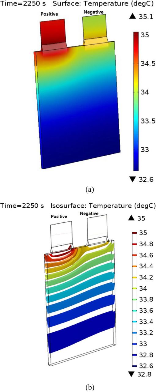
**Figure 10.** Temperature distribution at the end of 1.5 C discharge: (a) Surface tempeature (b) Isothermal surface in the battery core.

Fig. 11 shows the detailed battery dimensions and the thermocouple locations. PT and NT refer to the locations of thermocouples attached on the positive tab and negative tab, and #1∼#14 refer to the locations of thermocouples attached on the battery core surface.

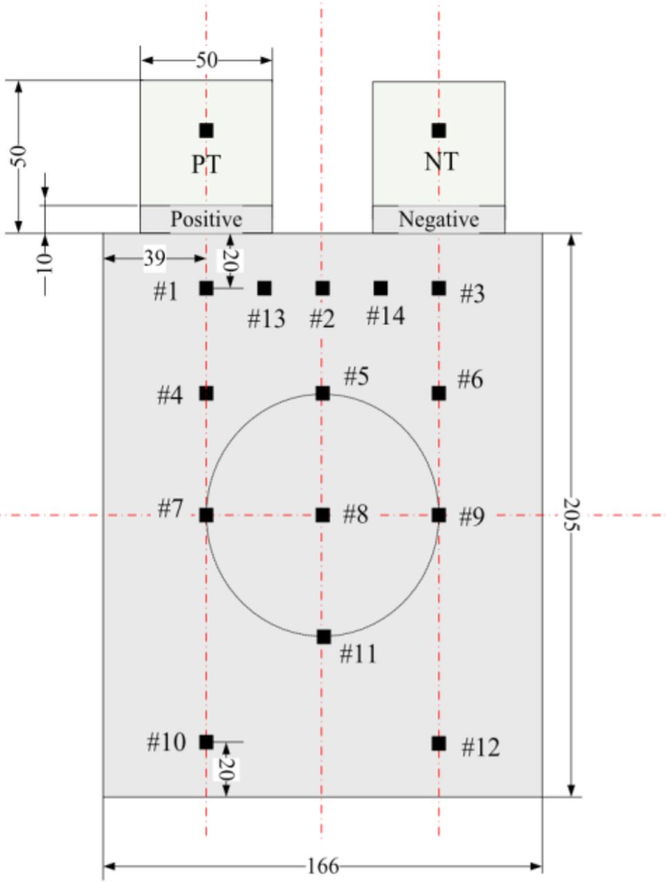
**Figure 11.** The dimensions of the cell and the locations of the thermocouples (unit: mm).

The validation experiment was conducted in an environment chamber. The chamber temperature was set at 25°C before the discharge experiment, and the battery was placed in the chamber for sufficient time to get thermal equilibrium. It is noted that the ventilation function of the chamber was shut down before discharging. Thus, the battery was in the natural convection environment without forced ventilation during the discharge. Similar natural convection environment is established for the estimation of convection heat transfer coefficient in Parameter determination section.

The specifications of the instruments used in the experiment are listed in Table IV.

Table IV. The specifications of the instruments.

Instrument	Specification
Cycler	MACCOR Series 4000
Environment chamber	Yashilin
Thermocouple	Type T; Precision: 0.1°C
Temperature recorder	National Instrument PXIe-4353

Fig. 12 depicts the temperatures recorded with the 16 thermocouples during 1.5 C discharge experiment. The temperatures of the tabs (PT and NT) follow quite different pattern compared with the temperatures of the battery core (#1∼#14). The temperature of the positive tab increases faster than any other locations owing to the comparatively larger ohmic resistance and contact resistance. As the temperature becomes high, the heat dissipation rate increases to slow down the rate of the temperature increase. The negative tab has a slower and smaller increase than the positive tab because of the lower electrical resistivity.

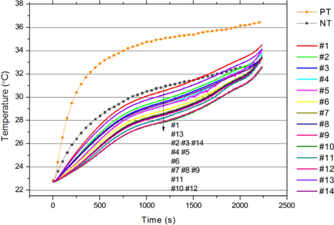
**Figure 12.** Temperature curves recorded by the 16 thermocouples during 1.5 C discharge.

Regarding the battery core, the temperatures increase almost linearly during 0∼750 s. After 750 s, the temperatures increase slowly due to the enhanced heat dissipation rate. However, the temperature increases at a high rate after 2000 s due to high resistance at low state of charge.

The temperature distribution demonstrates an approximately one-dimensional characteristic. Generally, the locations closer to the positive tab have higher temperature increase. The areas near the positive tab remain hottest during the whole discharge procedure. However, at the end of discharge, several locations far from the tab exhibit rapid temperature increase. This phenomenon can be attributed to the large current density at this area near the end of discharge. The current density distribution will be discussed in the following section.

Fig. 13 compares the simulated discharge curves with the experiment results for different C-rate operations. Good agreement is achieved between the experiment and simulation results.

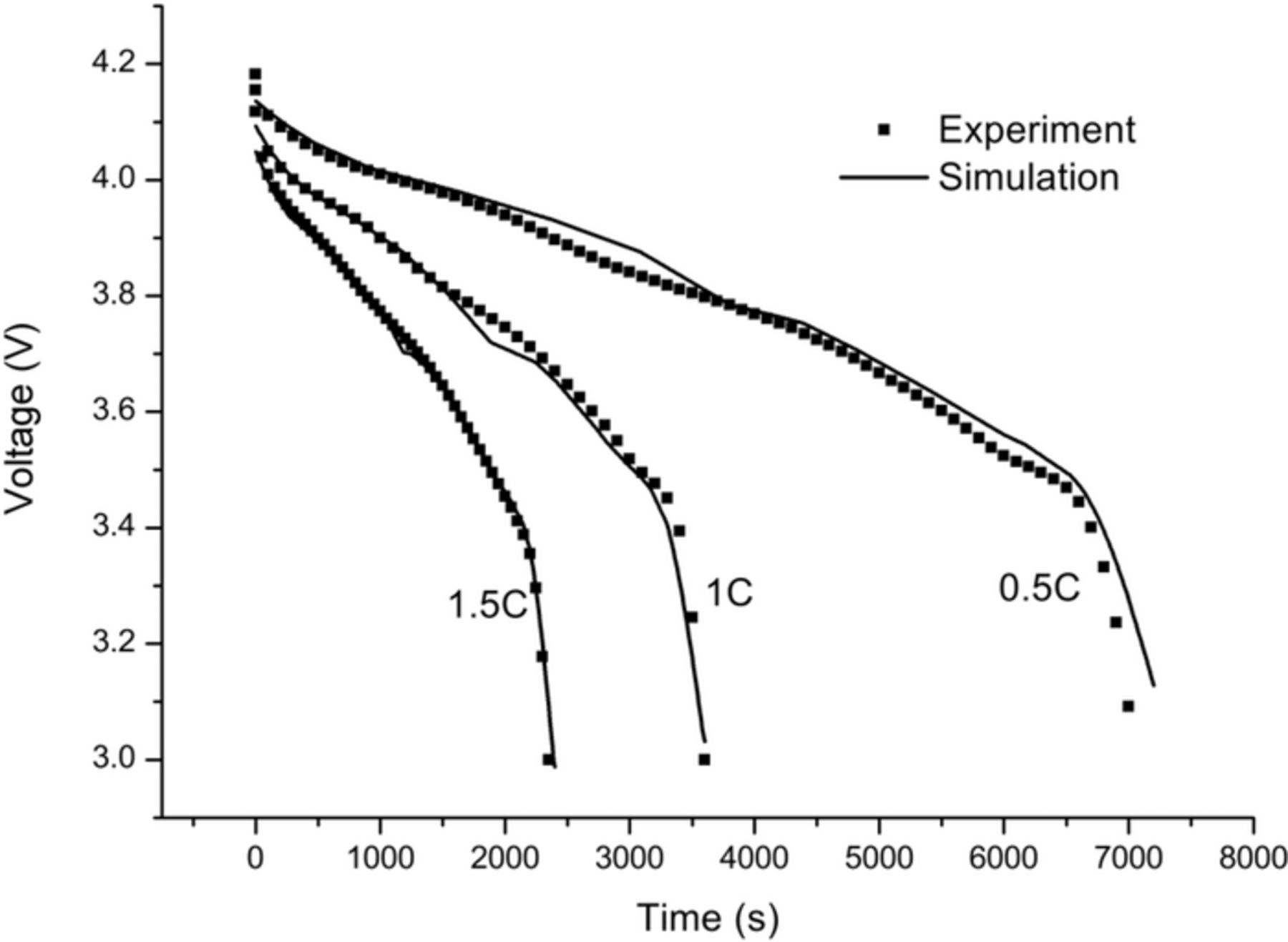
**Figure 13.** Simulated and experiment discharge curves.

Three representative locations on the diagonal of the battery core, #1, #8 and #12, were selected for the temperature validation. Fig. 13 compares the simulated and experimental temperatures at three locations. The comparison shows that difference between the experiment and simulation results is at largest 0.5°C.

Sensitivity analysis

Sensitivity analysis is used to quantify the influence of thermal parameters on temperature distribution. The normalized sensitivity coefficient is defined as

where θ is a thermal parameter, X is a chosen indicator for the temperature performance, including maximum temperature T_max and temperature variation ΔT. The first-order derivative in Eq. 21 was approximated with first-order difference in calculations. The normalized sensitivity coefficient reflects the impact of the thermal parameters on the temperature performance.

Several finite element simulations at a series of thermal parameters, as shown in Table V, were conducted to calculate the sensitivity coefficients according to the definition in Eq. 21.

Table V. Simulation cases to calculate the sensitivity coefficients.

	k_in	k_th	C_p	h_core	h_tab
Case	(W m⁻¹ K⁻¹)	(W m⁻¹ K⁻¹)	(J kg⁻¹ K⁻¹)	(W m⁻² K⁻¹)	(W m⁻² K⁻¹)
Base	21	0.48	1243	4	4
I	21*(1±10%)	0.48	1243	4	4
II	21	0.48*(1±10%)	1243	4	4
III	21	0.48	1243*(1±10%)	4	4
IV	21	0.48	1243	4*(1±10%)	4
V	21	0.48	1243	4	4*(1±10%)

The calculated results are listed in Table VI.

Table VI. Sensitivity coefficients of four thermal parameters.

Thermal parameter θ	η^T_max_θ	η^ΔT_θ
k_in	−1.5°C	−2°C
k_th	−0.1°C	−0.1°C
C_p	−5.5°C	1.0°C
h_core	−3.0°C	0.2°C
h_tab	−1.5°C	−1.1°C

All the sensitivity coefficients of the maximum temperature, η^T_max_θ, are negative. With the increase of these parameters, the capability of heat conduction (k_in and k_th), heat absorption storage (C_p) and heat removal (h_core and h_tab) improve, thereby reducing the maximum temperature.

The specific heat capacity C_p has the largest sensitivity affecting the maximum temperature and the in-plane thermal conductivity k_in has the largest sensitivity affecting the temperature variation. However, C_p and k_in are largely determined by the battery composition and structure. For the battery thermal management, only the h_core and h_tab are adjustable variables. h_core has larger influence in the maximum temperature while h_tab has larger influence in the temperature variation. With the increase of h_tab, both the maximum temperature and temperature variation decrease remarkably. The results imply that the thermal management of the pouch-type batteries should pay more attention to the convective cooling of the tab.

The results also provide insights into the required accuracy for the different thermal parameters. For instance, a 10% inaccuracy in the specific heat capacity leads to an error of 0.5°C (−5.5°C × 10%) to the maximum temperature and an error of 0.1°C (1.0°C × 10%) to the temperature difference. Compared with the difference between the simulation and experiment results shown in Fig. 14, the errors induced by the 10% inaccuracy in the specific heat capacity is negligible. Thus, 10% inaccuracy of the specific heat capacity is acceptable in the modeling.

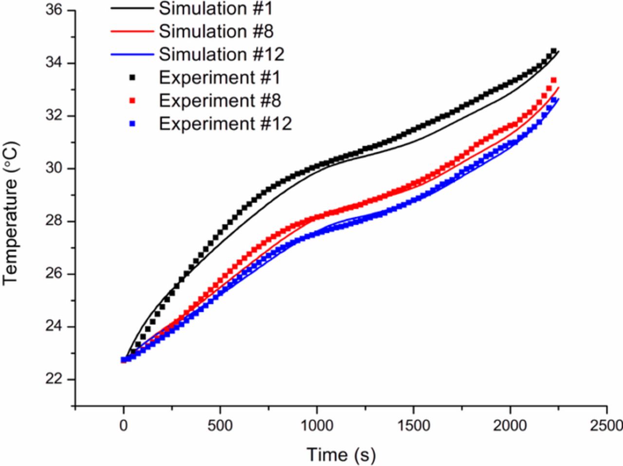
**Figure 14.** Simulated and experiment temperature curves at different locations during 1.5 C discharge.

The sensitivity coefficients listed in Table VI are used to explore the combined effect of different thermal parameter change. The maximum temperature and temperature variation at different sets of thermal parameters can be correlated using the sensitivity coefficients, as written in:

where T'_max and T_max are maximum temperatures for two sets of thermal parameters, ΔT' and ΔT are temperature variations for two sets of thermal parameters, Δθ_i is the difference of the thermal parameter θ_i, η^T_max_θ and η^ΔT_θ are the sensitivity coefficients.

The combined effect of h_core and h_tab is evaluated using the sensitivity analysis. Five sets of h_core and h_tab are listed in Table VII. The simulation results of the base set of provides the T_max and ΔT in Eqs. 22∼23. Other four sets have a 10% increase or decrease of the two convection heat transfer coefficients. The predicted T_max and ΔT using the sensitivity analysis and the simulated T_max and ΔT from the finite element model are compared in Table VII.

Table VII. The predicted T_max and ΔT from Eqs. 22∼23 and the simulated T_max and ΔT from finite element models for different sets of thermal parameters.

	Predicted	Simulated	Predicted	Simulated
	T_max(°C)	T_max(°C)	ΔT(°C)	ΔT(°C)
Base (h_core = h_tab = 4)		35.07		2.43
Set 1 (h_core = h_tab = 4.4)	34.62	34.65	2.34	2.32
Set 2 (h_core = 4.4, h_tab = 3.6)	34.92	34.94	2.56	2.57
Set 3 (h_core = 3.6,h_tab = 4.4)	35.22	35.19	2.30	2.27
Set 4 (h_core = h_tab = 3.6)	35.52	35.50	2.52	2.54

Table VII indicates that the predicted thermal performance agree quite well with the simulated results. Thus, the sensitivity analysis provides an effective method to evaluate the effect of changing thermal parameters without high computational cost. For the battery thermal design, the sensitivity analysis enables the battery designers to determine reasonable range of thermal parameters before high-cost simulation. For the battery thermal management, the sensitivity analysis is helpful to the online estimation of battery temperature at different cooling rate.

Discussion

The potential distributions in the positive electrode and negative electrode during discharge are shown in Fig. 15. The black arrows shown in Fig. 15 represent the potential gradient. There are very little variations of the electrode potential due to the high electrical conductivity of the current collector. However, potential gradients are evident in the areas near the tabs owing to the current divergence effect of the positive tab and the converge effect of the negative tab.

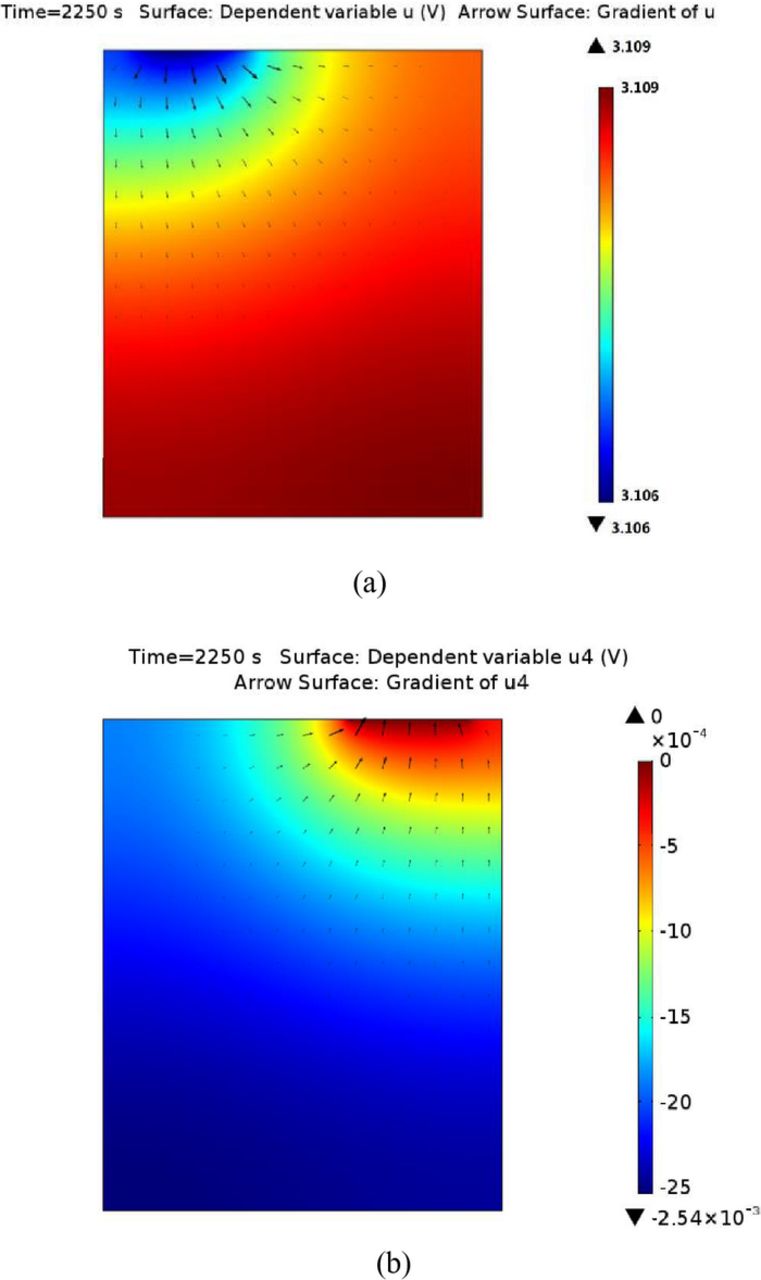
**Figure 15.** Potential distributions at the time of 2250 s in 1.5 C discharge: (a) Positive electrode (b) Negative electrode.

The distribution pattern for the current density changes drastically during the whole discharge procedure, as shown in Fig. 16. At the 200 s of the 1.5 C discharge, the current density is higher at the vicinity of the tabs. However, the current density at the bottom of the current collectors becomes larger at the end of the discharge, because the active material at the top side of the electrodes has been depleted in the earlier stage of the discharge.

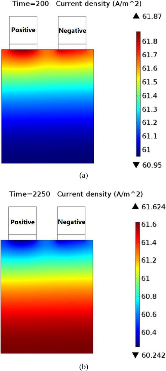
**Figure 16.** The transverse current density distribution for 1.5 C discharge at: (a) t = 200 s; (b) t = 2250 s.

Fig. 17 shows the distribution of the heat generation rate, which resembles the pattern of the transverse current density. It is concluded that the transverse current density is a dominant variable to determine the heat generation rate, as indicated in Eqs. 7∼10.

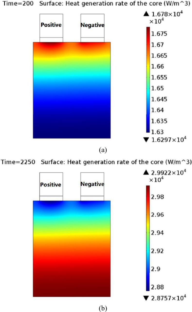
**Figure 17.** The heat generation rate distribution for 1.5 C discharge at: (a) t = 200 s; (b) t = 2250 s.

During the 1.5 C discharge, the heat generation rates at the locations of #1, #8 and #12 are shown in Fig. 18.

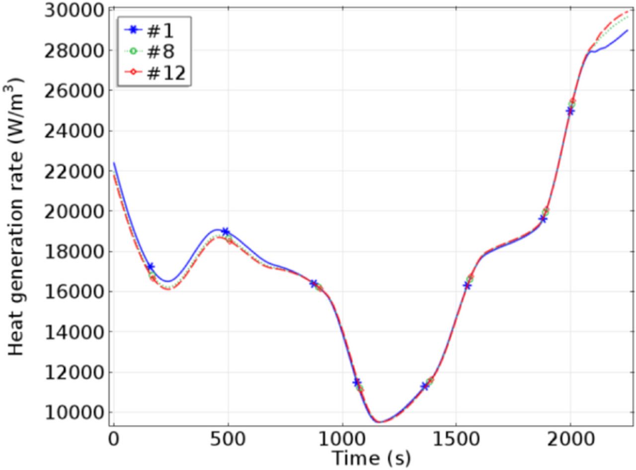
**Figure 18.** Minimum and maximum heat generation rates in the battery core during the 1.5 C discharge.

The evolution of the heat generation rate is attributed to the change of entropy coefficients and that of equivalent resistance. The decrease of the heat generation rate before 1200 s results from the lower resistance and the increase in the entropy coefficient at the SOC range of 0.5∼1.0, as shown in Fig. 7 and Fig. 9. The overpotential resistance shows a dramatic increase at low state of charge, thus the heat generation rate exhibit a rapid growth at the end of the discharge.

At the beginning of the discharge, #1 exhibits the largest heat generation rate due to the largest current density, as shown in Fig. 16 and Fig. 17. The variation of the heat generation rate between the three locations becomes smaller during 750∼2000 s. However, when it comes to the end of discharge, the heat generation rate of #12 becomes the largest, which coincides with the changing of the current distribution.

Fig. 18 shows that the heat generation rate changes greatly during the discharge, while the spatial variation of the heat generation rate is rather small.

To quantify the non-uniformity of the distribution, a dimensionless indicator is defined as

where X_max is the maximum of X, X_min is the minimum of X and X_average is the average of X. X can be referred to any distributed variable, such as temperature T. The calculated results of temperature, heat generation rate and current density are listed in Table VIII. As is clear from Table VIII, the non-uniformity of temperature distribution is much higher than the heat generation rate and the current density. The results indicate that the non-uniformity of the heat generation rate is not the only cause of the temperature distribution.

Table VIII. The range, average and non-uniformity indicator of different field variables.

Variable	Range	Average	Non-uniformity indicator
Temperature	32.7∼35.2°C	33.5°C	7.5%
Current density	60.2∼61.6 A m⁻²	61.0 A m⁻²	2.3%
Heat	2.88∼2.99	2.94 × 10⁴ W m⁻³	3.7%
generation rate	× 10⁴ W m⁻³

Heat flux from the tabs is another reason for the temperature distribution of the battery core. The Joule heat generation rate is 2.55 × 10⁵ W m⁻³ for the positive tab and 1.83 × 10⁵ W m⁻³ for the negative tab, both of which are one order of magnitude larger than the heat generation rate in the battery core. Both the experiment results in Fig. 12 and the simulation result in Fig. 10 show that the tabs are hotter than the core. Fig. 19 depicts the heat fluxes from the tabs to the core. The heat flux is proportion to the temperature gradient between the tab and the core. At the beginning of discharge, the heat generation rate of the core is much smaller than the tab. As a result, large temperature gradient exists in the vicinity of the tab, and the heat flux rises to the peak. The temperature gradient diminishes with the heat flux heating the core. Thus, the heat flux decreases after it reaches the peak. The positive tab has a larger heat flux due to the higher heat generation rate.

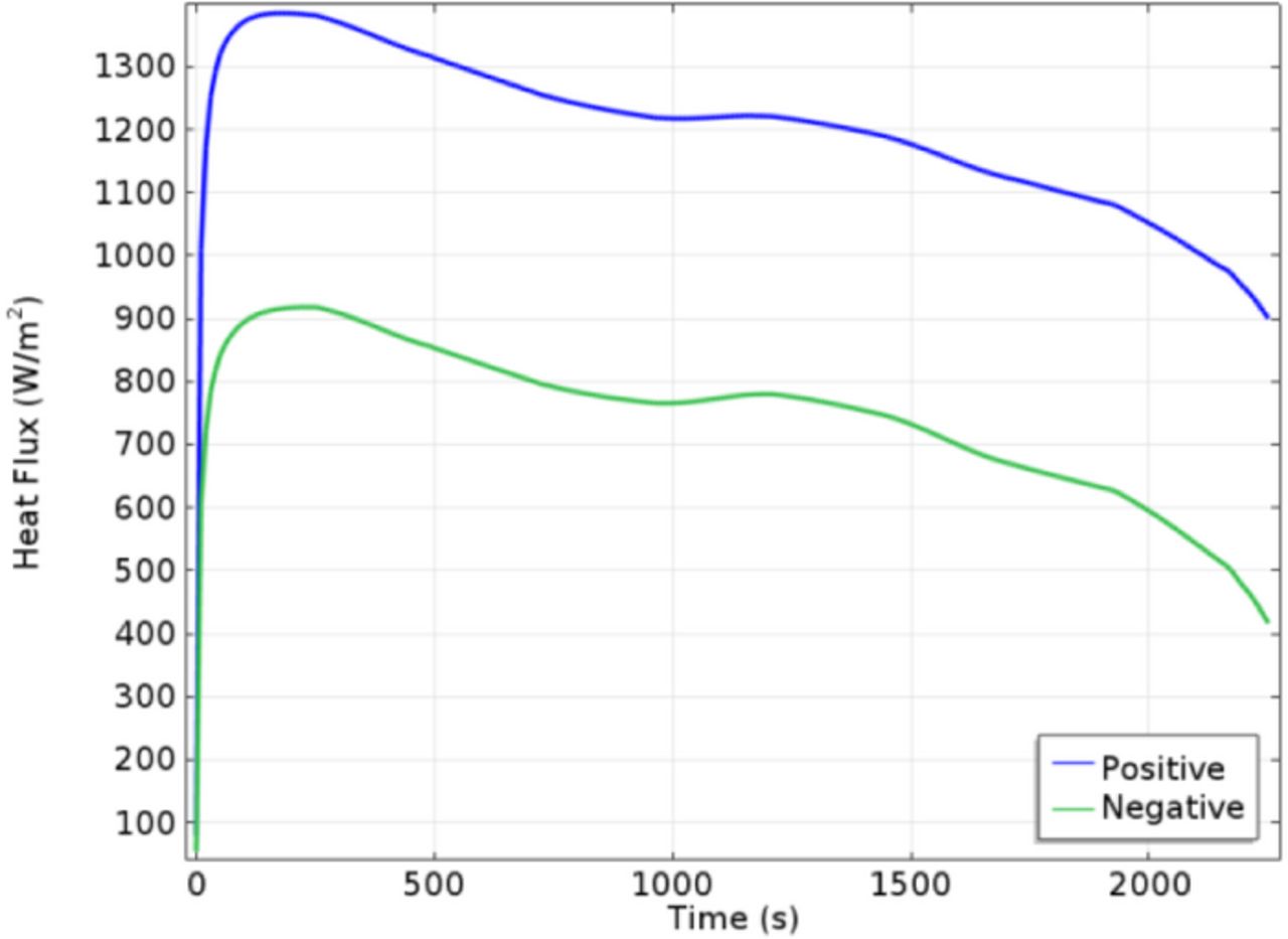
**Figure 19.** Heat fluxes from the positive tab and negative tab to the battery core.

Considering the both tabs are placed in the same electrode edge, the external heating effect from the tabs show great impact on the temperature distribution.

To further expose the influence of the tabs on the temperature non-uniformity, the temperature distribution of a thin-tab design was simulated using the present model. The thin-tab design differs from the original design only in the thickness of the tab: the thickness of the original tab is 0.3 mm, while that of the thin tab is 0.2 mm.

For the thin-tab design, the hot zone adjacent to the positive tab shows dramatically higher temperature than the original design, as shown in Fig. 20. The high temperature can be attributed to the increase in heat generation rate due to the increase in tab resistance, as indicated in Eq. 12. The maximum temperature of the thin-tab design is 43.9°C, which is 8.7°C higher than the original design. At the end of the discharge, the temperature difference of the thin-tab design is 8.1°C, which is 5.6°C higher than the original design.

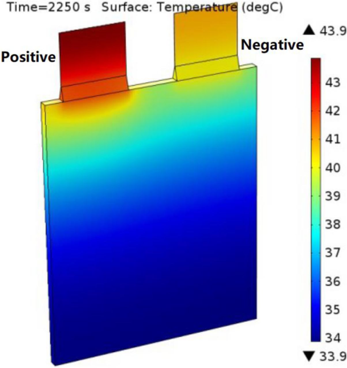
**Figure 20.** Temperature distribution at the end of 1.5 C discharge in the thin-tab design.

The deteriorated thermal performance is attributed to the increased heat generation rate of the tabs. As shown in Fig. 21, the heat fluxes from the tabs nearly double the heat fluxes of the original design shown in Fig. 19.

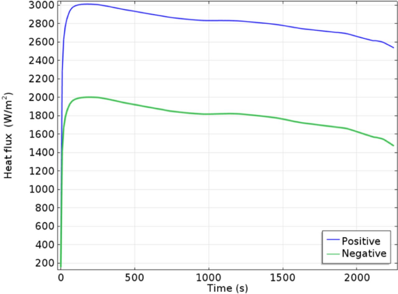
**Figure 21.** Heat fluxes from the positive tab and negative tab to the battery core in the thin-tab design.

Conclusions

In this study, a multi-dimensional thermo-electrical model was developed to study the thermal behavior of a large-format pouch-type lithium-ion battery. Key parameters are determined from carefully designed experiments to improve the modeling accuracy. Instead of the single-point temperature validation, the model was validated using temperatures measured with multiple thermocouples on the battery surface.

Employing the validated thermo-electrical model, a sensitivity analysis is conducted to evaluate the relative importance of the thermal parameters for the thermal performance. The specific heat capacity has the largest magnitude of influence on the maximum temperature, and the in-plane thermal conductivity has the greatest impact on the maximum temperature variation. In addition, the combined effect of adjusting different thermal parameters can be predicted using the sensitivity coefficients, which is cost-efficient and helpful for the battery thermal design and management. The main cause for the temperature non-uniformity throughout the battery is the heat flux from the tab, rather than the non-uniformity of the heat generation rate. The heat flux rises to the peak near the beginning of discharge, and maintains high level afterwards. The positive tab has a larger heat flux than the negative tab due to the larger heat generation rate. As a result, the area near the positive tab remains hottest during discharge. To investigate the importance of the tab, a hypothetical thin-tab battery is examined for comparison. The simulated maximum temperature and temperature variation of the thin-tab design are much higher than the original design.

Using the thermal modeling techniques introduced in this paper as a virtual tester for the effects of design parameters on the thermal performance, our group is developing a thermal design methodology for the large-format battery. The methodology includes the specification of the design criterions, design of experiments, surrogate model construction and global sensitivity analysis, etc. Appling the methodology, the thermal performance of the battery is optimized systematically. These results will be presented in Part II of the series of articles.

Acknowledgment

This work is supported by the National Natural Science Foundation of China under the grant number of 51207080, and Suzhou (Wujiang) Automotive Research Institute, Tsinghua University under the number of 2012WJ-A-01 and International S&T Cooperation Program of China under the grant number of 2013DFG60080.

Thermal Design for the Pouch-Type Large-Format Lithium-Ion Batteries: I. Thermo-Electrical Modeling and Origins of Temperature Non-Uniformity

Article metrics

Author affiliations

Author notes

Dates

Abstract