Abstract
In this work we demonstrate the validity of a multi-physics model using COMSOL to predict the local current density distribution at the cathode of a copper electrowinning test cell. Important developments utilizing Euler-Euler bubbly flow with coupled Nernst-Planck transport equations allow additional insights into deposit characteristics and topographies.
Export citation and abstract BibTeX RIS

This is an open access article distributed under the terms of the Creative Commons Attribution Non-Commercial No Derivatives 4.0 License (CC BY-NC-ND, http://creativecommons.org/licenses/by-nc-nd/4.0/), which permits non-commercial reuse, distribution, and reproduction in any medium, provided the original work is not changed in any way and is properly cited. For permission for commercial reuse, please email: oa@electrochem.org.
Electrowinning is the electrochemical process of depositing metal from dissolved metal ions without replacement of metal ions via anodic dissolution. This is an important method for a variety of primary and secondary metals processing scenarios. Of paramount operational importance is the topography of cathodic deposits. Irregularities in the form of surface perturbations (roughness, nodule formation), geometric inconstancies (misaligned, bent or tilted cathodes) are often the driving factors in short circuiting which influences current efficiency and the frequency of the harvest cycle, thereby impacting operational costs. This paper describes the fundamental methods of finite element analysis to determine the average thickness of a deposit in an electrowinning cell utilizing a multi-physics approach. The objectives of this approach are to facilitate the accurate prediction of local current density and the average cathodic thickness. The techniques to accomplish these objectives include transport via numerical simulation of the Nernst-Plank equation and fluid dynamics via Euler-Euler two phase flow.
To better understand the multi-physics nature of electrowinning systems Figure 1 of a copper system is provided. This schematic representation of a single anode cathode pair shows the major influences of the system. Copper is deposited at the anode via cathodic reactions. Oxygen is generated at the anode due to the counter reaction of water splitting. The evolution of oxygen bubbles contributes significantly to the agitation of the solution via buoyancy and slip-drag forces of bubble movement. Accurate modeling of solution density changes due to the copper depletion at the cathode is critical to the simulation. Diffusion, migration and bulk species transport combine to describe the movement and concentration of species of interest.
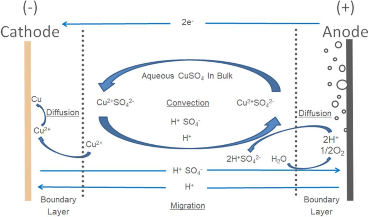
Figure 1. Schematic representation of a copper electrowinning cell. Note stoichiometry is unbalanced for illustrative purposes due to neglecting of complexation.
As covered in the review section there is ample opportunity for advancing the modeling of electrowinning systems. As such the focus of this paper will cover the development of the foundation of a 2D electrowinning Finite Element Model to study localized current distributions along the cathode. It will also present the experimental validation methods needed to produce results to compare to the model.
Review
To understand the mechanics of the model and to provide context for its development, a review of select literature is provided. Works specific to the field of electrowinning are covered by References 1–7 and 8–10. These papers represent work specific in the field of study from the mid-1980's to current.
Beginning in 1986 Ziegler et al.1–3 introduced a Euler–Euler type model where the local bubble gas fraction influences the liquid density. The system studied was a cadmium sulfate system. A RANS κ–l type was utilized to model turbulence with the more common κ– not fitting the experimentally determined velocities. Anodic bubble generation was determined via solving nodes of parallel resistors for the electrolyte where the y component of conduction was omitted due to the high aspect ratio of the cell. The effect of bubble on electrolyte conductivity was incorporated via the Bruggeman equation. This work although comprehensive in it's treatment of fluid dynamics did not include treatment of mass transport or electrode kinetics.
Philippe4 in modeling a hydrolysis cell pursues a different approach using the current density as a function of Ohm's Law with the current density vector being:
![Equation ([1])](https://content.cld.iop.org/journals/1945-7111/165/5/E190/revision1/d0001.gif)
where I is current, κ is conductivity and Φ is potential. The effect of gas interactions with conductivity is included using the Bruggman relation.4 The fluid flow equations used are of a Lagrangian nature with a force coupling term added to the base Navier–Stokes equation to produce the effect of bubbles.
Leahy et al.5 provides an excellent comparison of an electrowinning model to previous work. Convection and diffusion are modeled, but the effects of gas conductivity on the electrolyte are not considered. An Euler–Euler approach is utilized with gas fraction incorporation into fluid density with a κ–ω turbulence model. This work unlike that presented by Ziegler, assumed constant anodic current density. However, this work presents important advancements which include the consideration of copper concentration and the depletion at the cathode and resulting density effects on the flow.
Shukla et al.6,11 provide basis for the current study proceeding the current work under the same sponsorship. A copper sulfate electrowinning system is studied via design of experiments to determine a model for roughness. Failure analysis statistics are utilized to predict time to short. A COMSOL model is presented. The model utilizes Navier–Stokes transport and a volume force to simulate buoyancy forces from the anodic gas evolution.
Leahy et al.7 in an expansion of his previous paper utilizes a RANS–SST (Shear Stress Transport) for time averaged turbulent flow. The cathodic transport is handled based on the current density and transference number and Faraday expressions are used for anodic and cathodic generation. Thus the work commenced5 is enhanced by a change in the turbulence model and the incorporation copper transport utilizing the Schmidt number. Attention is paid to the transient nature of the fluid flow.
Najminoori et al.8 use a model that is very similar to that of Hemmati et al.16 with RANS Euler–Euler k-ω as the CFD (computational fluid dynamic) component and the same type of transport equation. Gas is produced at the anode according to the Faraday expression. This work is significant because it contains more than one electrode set.
Hreiz et al.9 provide a review of what they term "Vertical Plane Electrode Reactors with Gas Electrogeneration" or VPERGEs. This article focuses on the varying cell and fluid flow configurations surveyed. The literature with regard to bubble formation, properties and measurement techniques are covered. Models surveyed include a table listing the type of transport, turbulence and electrochemical coupling.
Hreiz et al.10 then present their own model after reviewing the literature in Ref. 9 with a Euler–Lagrange model validated with PIV (Particle image velocimetry). The cell was a double electrode gas generation type. Gas fractions and cell velocities were studied and captured. Additional modifications to the injection point were needed to reproduce key features. The numerical results were in general agreement with the experimentation. The use of the Euler-Lagrange method was to capture numerically the bubble dispersion without having to account for added volume forces.
From this body of work it can be seen that although fluid mechanic considerations appear to be represented, coupling of diffusion, migration, and convection via the Nernst–Planck equation with Buttler–Volmer electrode kinetics has not been performed.
Other works relevant to electrorefining and electrodeposition were also investigated for useful concepts and developments. These can be found in References 12–19. These provide examples of utilizing various combinations of Nernst–Planck transport equation with various types of electrode kinetics.
As identified in these two groups of work it appears that including the Nernst–Planck transport equation coupled with electrode kinetics and an Euler–Euler two phase CFD approach would be an novel and useful approach for describing a copper electrowinning system. As such, the objective of this work will be to present such a methodological framework and experimentally validate the modeled results via experimental. The works of Free20 and Newman21 were also heavily drawn from for inspiration and clarification of electrochemical principles.
Methods
The methods utilized in this study fall under two broad categories. The first is the theory and creation of a finite element electrowinning model. The second is the strategy used to validated the model. The research was primarily conducted using COMSOL 5.2a.
Geometry
A test cell was designed and fabricated to produce copper deposits for model validation. The test cell is shown in Figure 2.
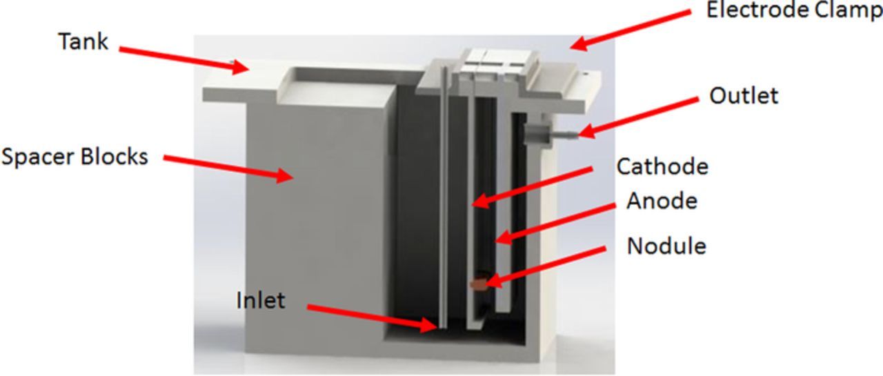
Figure 2. Rendering of test cell showing major components of electrowinning test cell.
Figure 3 shows the general layout of the cathode and anode pair with shielding and key dimensions. The model was simplified to a 2D geometry because of planer electrodes. It is assumed that the centerline of the cell as represented by section AA in Figure 3 represents a plane of symmetry and as such the 2D infinite width holds true. The geometric representation in COMSOL is shown in Figure 4.
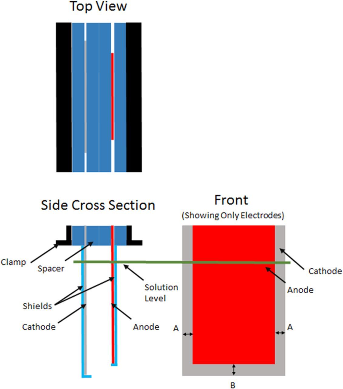
Figure 3. Typical cathode and anode arrangements. The cathode as placed in solution measures approximately 0.170 m tall by 0.140 m wide. The anode is approximately 0.155 m tall by 0.102 m wide. Dimension A in is 18.5 mm and dimension B is 16 mm. The cathodic recess and shield edge thickness are all 1/4 inch. The electrolyte level is 0.170 m above the bottom of the cathode.
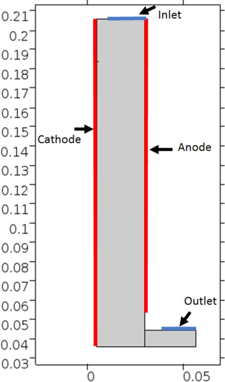
Figure 4. Geometry as represented in COMSOL multiphysics. Units in m.
Fluids
Critical to the validity of the model are determining suitable expressions for critical parameters such as density and viscosity.
Density
The equation used for density was a modified form of an equation provided by Price et al.22 and it is shown as Equation 2.
![Equation ([2])](https://content.cld.iop.org/journals/1945-7111/165/5/E190/revision1/d0002.gif)
where, ρ is in kg/m3, CCu is in mol/m3, CH2SO4 is in kg/m3, MwCu is in kg/mol, T is in °C. The fit of the data to the expression is shown in Figure 5.
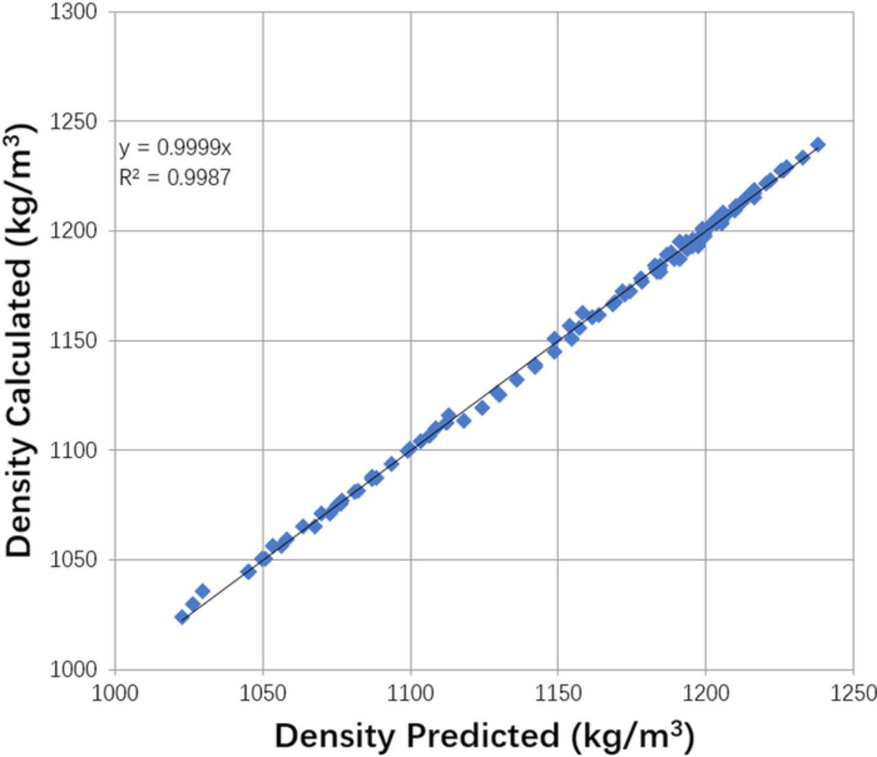
Figure 5. Density model fit. Equation modified from that presented in Reference 22.
This equation is applied across the electrolyte domain, and varies with the concentration of Cu2 +.
Viscosity
The equation for dynamic viscosity was determined by linearizing the temperature term and performing linear regression from data obtained from Price et al.22
![Equation ([3])](https://content.cld.iop.org/journals/1945-7111/165/5/E190/revision1/d0003.gif)
where μ is the dynamic viscosity in Pa · s, CCu is the localized cupric ion concentration in mol/m3, MwCu is in kg/mol, and CH2SO4 is the initial  concentration in kg/m3. The fit of experimental to model is shown in Figure 6. This equation is also applied across the electrolyte domain, varying with the concentration of Cu2 +.
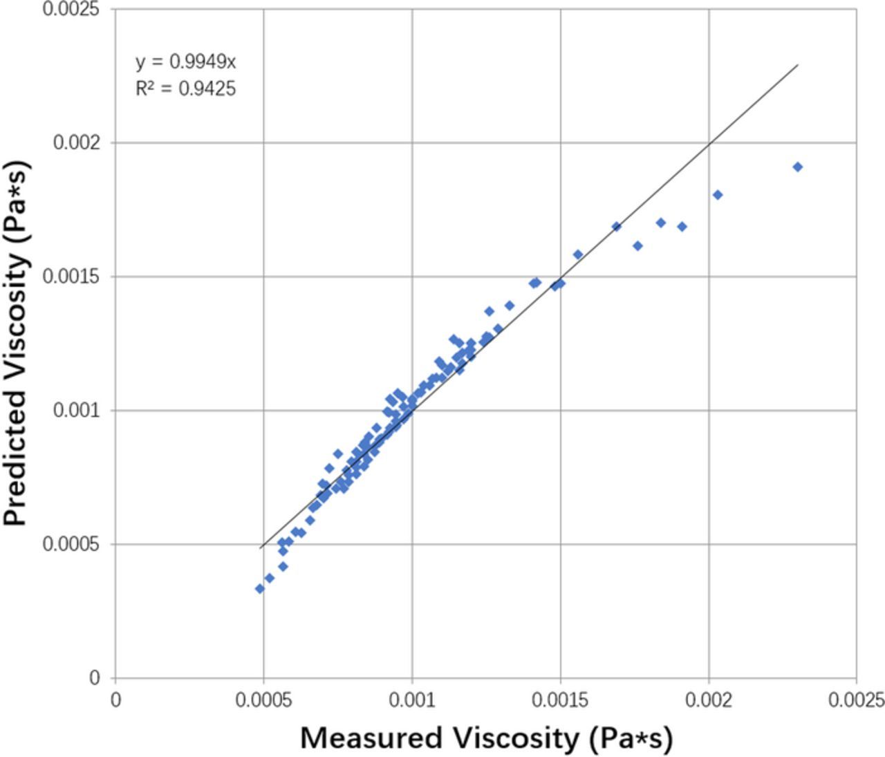
Figure 6. Viscosity model fit. Equation empirically fit from data presented in Reference 22.
Parameters
In addition to fluid parameters, physical phenomena such as species activity and diffusion must be considered. In concentrated electrolytes more complicated activity calculation methods must be used.20
Activity model
Activities are given by the following expression 4:
![Equation ([4])](https://content.cld.iop.org/journals/1945-7111/165/5/E190/revision1/d0004.gif)
where, aj is the activity of species j and is unit-less, γj is the activity coefficient, mj is the concentration of species j, m0is the reference concentration.
Only the species involved in the reaction affect the potential. However, all species in an ionic solution affect the "thermodynamic concentration" known also as activity. This modification occurs through the use of the activity coefficient.
Most fundamental formulas for the determination of activity coefficients have been determined for dilute electrolytes. Increasing discrepancies arise for more concentrated solutions (I > 0.1) like those found in electrowinning cells. Literature was reviewed for a suitable high concentration expression. The work of Samson further modified the Davies equation to produce a more accurate expression than that of Pitzer. The following is the equation from Sampson et al.23,24
![Equation ([5])](https://content.cld.iop.org/journals/1945-7111/165/5/E190/revision1/d0005.gif)
where I is the ionic strength of the solution, which is calculated using Equation 6:
![Equation ([6])](https://content.cld.iop.org/journals/1945-7111/165/5/E190/revision1/d0006.gif)
zi is the charge of a given ionic species and N is the total number of ionic species in the acqueous solution. In Equation 5, A and B are temperature-dependent parameters, given by Equations 7 and 8:
![Equation ([7])](https://content.cld.iop.org/journals/1945-7111/165/5/E190/revision1/d0007.gif)
![Equation ([8])](https://content.cld.iop.org/journals/1945-7111/165/5/E190/revision1/d0008.gif)
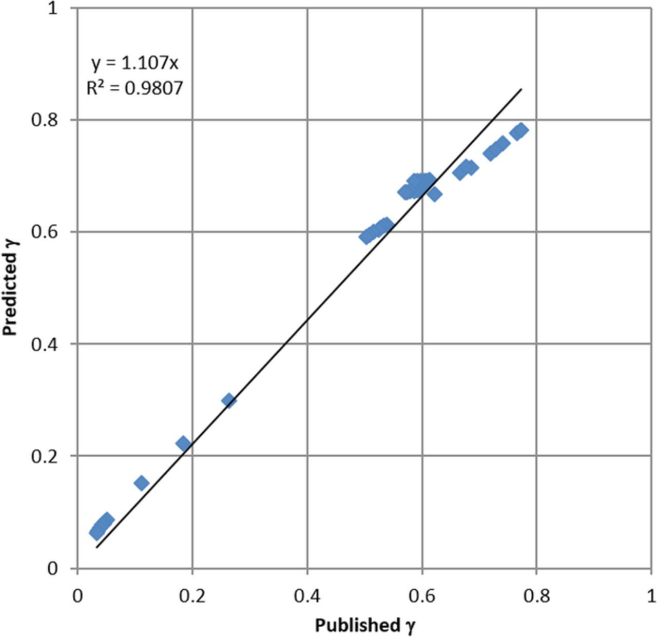
where F is the Faraday constant, 0 is the electrical charge of one electron and = r0 is the permittivity of the vacuum, R is the ideal gas constant and T is the temperature. Finally, the parameter ak in Equation 5 is related to the ionic radius and is specific to the ionic species. The results of the extended Davies models are compared as shown in Figure 7.
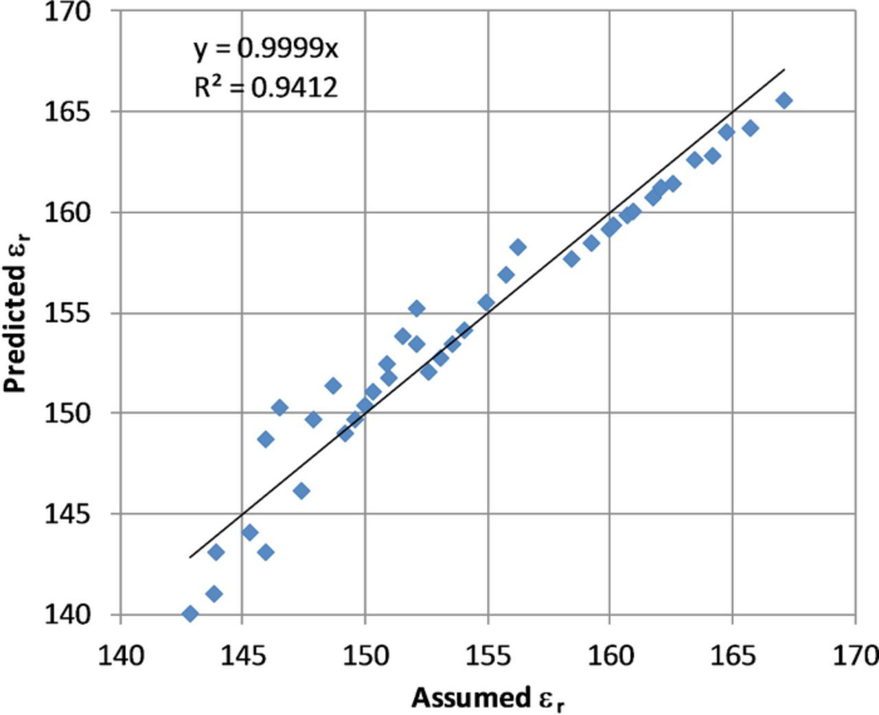
The model requires both the ionic radius and the dielectric constant. In order to supply the dielectric constant, an expression was derived from the data supplied in Reference 24. The premise was that the dielectric constant is a function of ionic strength and ionic radius.
![Equation ([9])](https://content.cld.iop.org/journals/1945-7111/165/5/E190/revision1/d0009.gif)
where, r is dielectric constant (unitless); I is ionic strength, mol/m3; ak is ionic radius in m; z is charge of species. To verify this equation the results were compared to the data provided in Reference 24 as shown in Figure 8. Use of the empirical fit dielectric equation showed reasonable agreement with the data provided.
Diffusion coefficients
Diffusion Coefficients for copper were calculated using the work of Moats et al.25 The work of Moats et al. was reviewed and regression was utilized to develop the following expression:
![Equation ([10])](https://content.cld.iop.org/journals/1945-7111/165/5/E190/revision1/d0010.gif)
where D2 +0, Cu is in cm2/s,  and Ci, Cu are the initial concentrations in mol/m3, MwH2SO4 and MwCu are in kg/mol, T is temperature in K. This equation has the following range: Ci, Cu = 35 − 60 (g/L),
  (g/L), T = 40 − 65°C. This expression demonstrates a reasonable fit of the data.
The diffusion coefficient in this model is set as a constant over the electrolyte domain for D2 +0, Cu. This assumption was made from the data being generated from a rotating disk electrode via the Levich equation. As such, the diffusion coefficient takes into account the overall effect of the boundary layer concentration and other effects. The diffusion coefficient is utilized by the model in the same way.
For SO2 −4 the diffusion coefficient was calculated by solving for the ionic radius using the Stokes-Einstein relation with a initial value of 1.065 × 10− 9 cm2/s in 25°C water. This was then modified via viscosity for electrolyte for use in the model.
Electrochemical model
Governing equations
To model the electrodeposition process in this study, the Tertiary Nernst-Planck interface was utilized to solve for the electrolyte potential (Φl), the current density distribution (il), and the concentrations of various species (Ci).26 A set of governing equations was used and solved.21, 26 In electrolyte, the governing equation for mass transfer in solution is the Nernst-Plank equation:
![Equation ([11])](https://content.cld.iop.org/journals/1945-7111/165/5/E190/revision1/d0011.gif)
where Ni, zi, ui, Ci, Di are the flux density, charge, mobility, concentration, and diffusivity of species i, F is Faraday's constant, ∇Φl is an electric field, ∇Ci is a concentration gradient, and ν is the velocity vector.
Because there are no homogeneous reactions in the electrolyte, the material balance is governed by the equation:
![Equation ([12])](https://content.cld.iop.org/journals/1945-7111/165/5/E190/revision1/d0012.gif)
In the electrolyte, the current density is governed by:
![Equation ([13])](https://content.cld.iop.org/journals/1945-7111/165/5/E190/revision1/d0013.gif)
where ielectrolyte is the current density in the electrolyte, and other variables are defined previously. Due to the electroneutrality of the electrolytic solution, the last term on the right is zero (∑ziCi = 0). Therefore,
![Equation ([14])](https://content.cld.iop.org/journals/1945-7111/165/5/E190/revision1/d0014.gif)
On the electrodes, the current density is governed by Ohms Law:
![Equation ([15])](https://content.cld.iop.org/journals/1945-7111/165/5/E190/revision1/d0015.gif)
where is is the current density at the electrode, σs is the conductivity of the electrode and ∇Φs is an electric field. With conservation of current in the electrolyte and electrodes, we have:
![Equation ([16])](https://content.cld.iop.org/journals/1945-7111/165/5/E190/revision1/d0016.gif)
where k denotes an index that is l for the electrolyte and s for the electrode, and Qk is a general current source term and was zero in this model.27 Therefore, Eq. 16 becomes:
![Equation ([17])](https://content.cld.iop.org/journals/1945-7111/165/5/E190/revision1/d0017.gif)
At the electrode-electrolyte-interface, the overpotential η is defined as:
![Equation ([18])](https://content.cld.iop.org/journals/1945-7111/165/5/E190/revision1/d0018.gif)
where Φs is the electric potential of the electrode, Φl is the potential of the electrolyte adjacent to the electrode.
The current density in the electrolyte adjacent to the electrode has the following relationship with the local current density term in a modified form of the Butler-Volmer Equation 19:27
![Equation ([19])](https://content.cld.iop.org/journals/1945-7111/165/5/E190/revision1/d0019.gif)
where iloc is the local current density at the interface (also called the charge transfer current density), i0 is equilibrium exchange current density, CR, S is the surface concentration reduced species, CR, B is the bulk concentration of the reduced species, CO, S is the surface concentration of the oxidized species, CO, B is the bulk oxidant concentration of the oxidized species, αa is the anodic symmetry factor, αc is the cathodic symmetry factor, z is the number of electrons transferred in the rate limiting step (typically 1), F is the Faraday constant, R is the gas constant, T is the absolute temperature, and η is the overpotential.
The current density in the electrolyte adjacent to the electrode has the following relationship with the local current density term in the Butler-Volmer equation:27
![Equation ([20])](https://content.cld.iop.org/journals/1945-7111/165/5/E190/revision1/d0020.gif)
where i is the current density in the electrolyte at the interface, n is the unit normal vector to the electrode surface, and iloc is the local current density. See subsequent sections for additional details for cathode and anode kinetics.
Electrolyte species considered
A review of the literature show that the Copper Sulfate Acid system is complex and dissociates into a number of species. For simplicity the species considered in this work are Cu2 +, H+ and HSO−4. The excess sulfate from the copper dissociation is assumed to become bisulfate. The concentrations of each of these species are set initially with no generation due to heterogeneous chemical reactions between species.
Equilibrium potential
In order to determine cell voltages the equilibrium potential of both the anodic and cathodic reactions needed to be calculated. The equilibrium potential or E is given by the Nernst Equation 21:
![Equation ([21])](https://content.cld.iop.org/journals/1945-7111/165/5/E190/revision1/d0021.gif)
This equation uses the standard thermodynamic potential along with the product and reactant activities to determine the equilibrium potential for a half-cell reaction.
Effects of bubbles
The effect of diffusion is modified by the presence of oxygen bubbles formed at the anode. For this work the approach is to make diffusion modification a function of gas fraction in the electrolyte. Table I shows several equations for this purpose. These were adapted from the work of Hammoudi et al.29 which originally represented conductivity as a function of gas fraction. The selection of any of these equations at gas fractions <0.1 is rather arbitrary as there is little variation.
Table I. Diffusion modification based on gas fraction.29
| Relative Diffusion | Author |
|---|---|
 |
Rayleigh |
 |
Maxwell |
 |
Tobias |
| D = D0(1 − )1.5 |
Bruggeman |
| D = D0(1 − 1.5 + 0.52) |
Prager |
In this work the Maxwell equation form Table I was utilized. This allows variation of both diffusivity and migration. Hence, the changes in electrolyte conductivity and its effects can be considered as a function of dispersed gas bubbles in the electrolyte.
Migration was modeled by relating mobility to diffusion using the Nernst-Einstein relation:
![Equation ([22])](https://content.cld.iop.org/journals/1945-7111/165/5/E190/revision1/d0022.gif)
Cathode kinetics
For simplification in this paper it is assumed that copper is deposited on the cathode according to the following chemical reaction 23:
![Equation ([23])](https://content.cld.iop.org/journals/1945-7111/165/5/E190/revision1/d0023.gif)
However, for kinetics it is understood that the reaction above proceeds in two steps which are:
![Equation ([24])](https://content.cld.iop.org/journals/1945-7111/165/5/E190/revision1/d0024.gif)
![Equation ([25])](https://content.cld.iop.org/journals/1945-7111/165/5/E190/revision1/d0025.gif)
Accordingly, Newman21 in reviewing Mattsson and Brokris30 proposes (26):
![Equation ([26])](https://content.cld.iop.org/journals/1945-7111/165/5/E190/revision1/d0026.gif)
where, Cr is metallic copper and equal to 1, Co = C2 +Cu/CuBulk2 +, αa is the anodic charge transfer coefficient, αc is the cathodic charge transfer coefficient, io is the exchange current density. η is the over voltage calculated by the difference between the equilibrium potential and the electrode potential.
In reviewing this work in light of Newman's equation for the copper reaction21 it was determined that appropriate cathodic and anodic charge transfer coefficients are 0.545 and 1.455, respectively. For the exchange current density the following Equation 27 was used:30
![Equation ([27])](https://content.cld.iop.org/journals/1945-7111/165/5/E190/revision1/d0027.gif)
where, iof is the exchange current density at the desired concentration, ioi is the exchange current density at the reference concentration, aCuf is the final activity, aCui is the reference activity at ioi, β is the symmetry factor. From the works cited above ioi is set at 1 mol/l was 100 A/m2.
From the literature cited the copper reaction is based on Cu2 +. However, thermodynamics indicate that CuHSO+4 is the dominant copper species. It is assumed that in the boundary layer the CuHSO+4 dissociates into copper ions and bisulfate ions. Therefore, for simplicity, the cathodic flux reaction is likely to proceed according to Equation 28.
![Equation ([28])](https://content.cld.iop.org/journals/1945-7111/165/5/E190/revision1/d0028.gif)
This is important because it reduces the migration current carried bu copper species due to the change in charge from Cu2 +.
Anode kinetics
For the anodic reaction the work of Laitinen31 was referenced. This work represents experimental determination of io at different temperatures on a Pb-PbO2 electrode. Figure 9 shows the effect of temperature on io. The data from Figure 9 were used to develop Equation 29. It is important to note that logarithmic expressions were attempted, but were not as accurate as this expression.
![Equation ([29])](https://content.cld.iop.org/journals/1945-7111/165/5/E190/revision1/d0029.gif)
where, i0 is the exchange current density in A/m2, T is temperature in K.
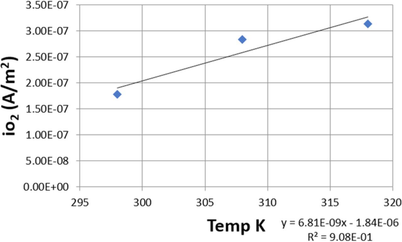
Figure 9. Anodic exchange current density versus temperature.
The anodic reaction is assumed to be:
![Equation ([30])](https://content.cld.iop.org/journals/1945-7111/165/5/E190/revision1/d0030.gif)
Bubbly flow
The form of the bubbly flow (BF) equations used assumes that the fluid is noncompressible and utilizes the following additional assumptions:32
- The gas phase density is insignificant compared to the liquid phase density
- The motion between the phases is determined by a balance of viscous and pressure forces
- Both phases are in the same pressure field
- Low gas concentration is low
- Turbulence is not modeled
The resulting Equation 31 from COMSOL is:28
![Equation ([31])](https://content.cld.iop.org/journals/1945-7111/165/5/E190/revision1/d0031.gif)
The continuity Equation 32 simplified via the low gas concentration assumption (ϕg < 0.01) is:
![Equation ([32])](https://content.cld.iop.org/journals/1945-7111/165/5/E190/revision1/d0032.gif)
The gas phase velocity 33 is given by:
![Equation ([33])](https://content.cld.iop.org/journals/1945-7111/165/5/E190/revision1/d0033.gif)
where ui represents the velocity vector of the specified component.
ul is the velocity vector
p is the pressure
ϕl is the phase volume fraction
ρl is the density
g is the gravity vector
F is any additional volume force
μl is the dynamic viscosity of the liquid
μT is any additional volume force
I is the identity matrix
The density of the gaseous phase is derived from the ideal gas law for oxygen. The slip model is of the pressure-drag balance type and the drag coefficient is from the Hadamard-Rybczynski model for small spherical bubbles.
Numerical approach
The governing equations have been discussed previously. In this section the boundary and initial conditions will be presented. Figure 4 shows the main boundaries, being inlet, outlet, anode or cathode. The remaining unspecified boundaries are zero flux or zero as the equations require.
For the Nernst–Planck equation the typical boundary condition is no convective species flux as shown by Equation 34.
![Equation ([34])](https://content.cld.iop.org/journals/1945-7111/165/5/E190/revision1/d0034.gif)
where n is the normal vector and Ni is the species flux. These boundary conditions apply for all species except copper. For copper, the inlet the concentration is fixed as a constant at the electrolyte makeup concentration and outlet conditions shown by Equation 35.
![Equation ([35])](https://content.cld.iop.org/journals/1945-7111/165/5/E190/revision1/d0035.gif)
where Di is the diffusion of species i and ci is the concentration of species i. For the anode and cathode, boundaries are given in Equation 36.
![Equation ([36])](https://content.cld.iop.org/journals/1945-7111/165/5/E190/revision1/d0036.gif)
where νi is the stoichiometric coefficient of species i, in this case given to be 0.96 due to current efficiency, iloc is the local current density and n F are the number of electrons in the reaction and Faraday's constant respectively.
For fluid boundaries, no slip conditions (velocity=0) exist except the inlet and outlet which are defined. For the purpose of this model the cathodic boundary is stationary with respect to time. Thus, no deformation of the domain occurs and fluid structure interactions are not considered.
As this is a transient model running to quasi-steady state, all species concentrations are given by the electrolyte bulk concentrations at time zero. The electrode current density is set to zero and ramps to run conditions to allow model convergence.
Experimental Validation
Experimentation
Current density determination from deposi-tion
As mentioned in Geometry section a test cell was created to produce deposits for model validation. Several different geometries were used to provide a range of comparisons. Figure 10 shows three different electrode configurations used for validation. These were selected as a representation of typical geometric occurrences in tank houses. Direct comparison of effective current density is obtained by numerical integration of the obtained deposit. The comparison of current densities between the deposit and that of the model was a key to the evaluation. Thickness is converted to current density via the expression 37.
![Equation ([37])](https://content.cld.iop.org/journals/1945-7111/165/5/E190/revision1/d0037.gif)
where iloc is the local current density, thkloc is the local thickness, n is the number of participating electrons, F is Faraday's constant, ρ is density, t is time, Aw is atomic weight. Further, by numerically integrating via expression 38 the average current density is obtained.
![Equation ([38])](https://content.cld.iop.org/journals/1945-7111/165/5/E190/revision1/d0038.gif)
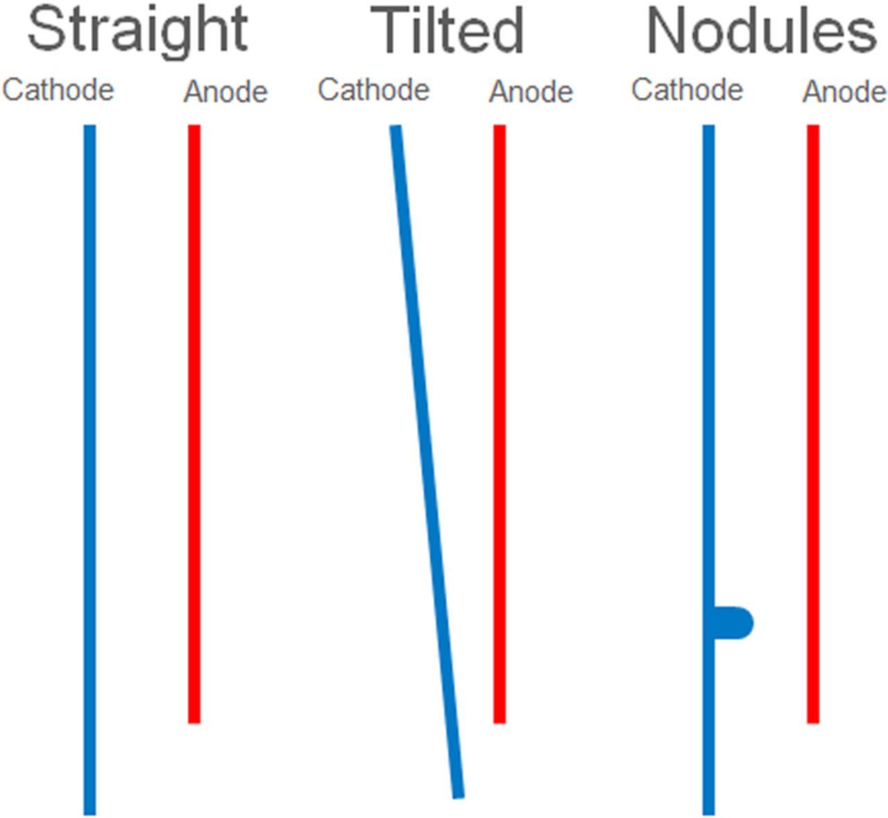
Figure 10. Electrode geometries used for validation.
The geometric parameters of the test cell and model are covered in Tables II–IV.
Table II. Straight cathode model geometric parameters.
| Parameter | Dimension (m) |
|---|---|
| Cathode height | 0.170 |
| Shield length beyond anode | 0.0064 |
| Anode to cathode gap | 0.02467 |
| Anode length | 0.155 |
| Cathode shield to tank | 0.0297 |
Table III. Titled cathode model geometric parameters.
| Parameter | Dimension (m) |
|---|---|
| Cathode height | 0.170 |
| Shield length beyond anode | 0.0064 |
| Anode to cathode gap | 0.02467 |
| Anode length | 0.155 |
| Cathode shield to tank | 0.0297 |
| Bend angle | 6.2773 (deg) |
Table IV. Nodule cathode model geometric parameters.
| Parameter | Dimension (m) |
|---|---|
| Cathode height | 0.170 |
| Shield length beyond anode | 0.0064 |
| Anode to cathode gap | 0.02467 |
| Anode length | 0.155 |
| Cathode shield to tank | 0.0297 |
| Nodule diameter | 0.009525 |
| Nodule length | 0.0127 |
| Nodule position | 0.033 |
The cathode height corresponds to the length of the cathode in the electrolyte. The shield recess is the set back distance from the edge of the cathode shield to the cathode surface. The shield thickness is the width of the shielding around the cathode. Anode to cathode gap is the distance between the anode and cathode. For the tilted cathode geometry the anode to cathode gap in Table IV is the largest gap between the anode and cathode at the top of the cell. The bend angle is the angle that the cathode was bent. Anode length is the length of the anode in the electrolyte. Cathode shield to tank is the distance from the bottom of the tank to the lower part of the cathode shield. In the model this distance is omitted and the bottom of the cathode is modeled as the bottom of the tank. For the nodule cathode described in Table IV the additional dimensions of nodule diameter, nodule length and position (from the bottom of the cathode to the centerline of the nodule) are included.
In order to capture the deposit thickness two different 3D scanners were utilized. For the straight and tilted cathode the NextEngine 3D scanner was utilized with a resolution of 0.127 mm. However, due to the nature of taking multiple scans and merging them into a composite, the spacial resolution is expected to be less. The other scanner utilized was Artec Spider 3D Scanner. This is a hand held unit that features better accuracy with a point accuracy to 0.05 mm. However, in practice due to the nature of surface roughness the filtering algorithm removed some of the feature roughness. Comparison between the roughness in the experimental current density figures in Results and discussion section show what appears to be roughness differences from the straight and tilted cathode results to the nodule cathode. These differences are due to the difference in 3D scanner capture and filtering.
The 3D data were imported to MeshLab allowing the raw mesh to be cleaned and simplified. This is an important step as Solidworks has a limit of 90,000 faces for an .stl file import. In addition the mesh was translated and rotated to achieve proper axis alignment. In Solidworks a perpendicular plane was created and the intersection with the mesh generated the 2D profile that the current density was calculated from.
Experimental setup
As shown in Figures 2, 3 and 4, the electrodes incorporated shielding and were arranged to represent the configuration shown in Figure 10 to evaluate the effects of straight, tilted cathodes and nodules on current local current efficiency.
To achieve cost effective replenishment of the copper in solution a system was developed. As shown in Figure 11 the cell resides in a bath held under isothermal conditions. The cell volume with spacers is 4.6 L and the level is maintained by an overflow port. The temperature of electrolyte is maintained at 40°C by an isothermally controlled (68 °C) water bath around the cell. The temperature difference is due to the insulative nature of the tank and the incoming temperature and flow rate of the electrolyte. Figure 12 shows the test cell setup in the water bath.
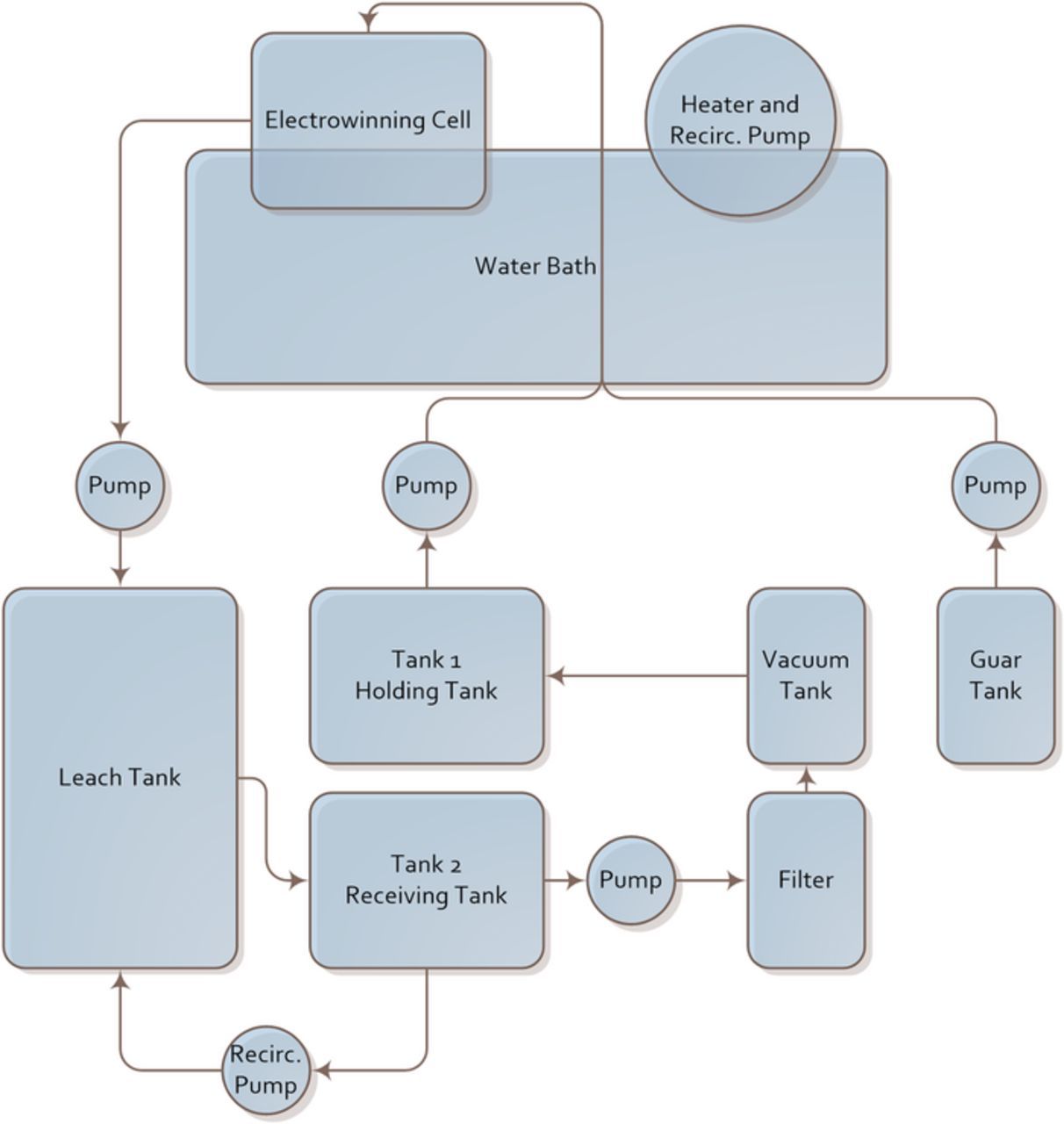
Figure 11. Copper replenishment leaching setup.
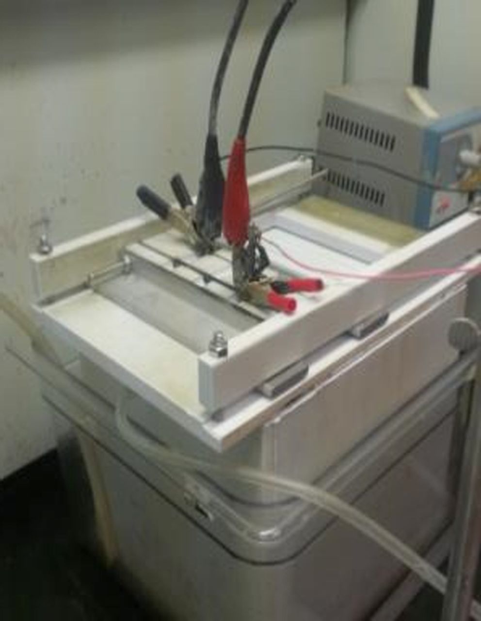
Figure 12. Electrowinning test cell setup.
Electrolyte is pumped from the holding barrel to the cell (see Figure 11). The overflow is collected in the copper dissolution vessel, which is filled with copper turnings. The dissolution vessel is a shallow vessel tilted at a slight angle to allow gravity based feeding of the electrolyte. The electrolyte from the electrowinning cell flows into the bottom of the upper end of the dissolution vessel to allow flow through the turnings. The turnings are kept damp with the electrolyte to facilitate oxidation and dissolution of the copper turnings. In addition a recirculation loop in the leaching system was added to further increase the concentration of copper should it be required. This recirculation is fed via drip lines on top of the copper to further increase the solution exposure to the copper which is dampened by electrolyte.
Copper concentration is checked once per day using open circuit potential measurements with a multimeter. The open circuit potential measurements were calibrated by utilizing solutions of know concentration to determine a calibration curve. Additional copper dissolution is performed as needed. The copper utilized was copper turnings 99+% pure from Flinn Scientific model C0089. The copper enriched solution is collected in the receiving barrel before being filtered. The solution is then returned after filtration to the holding tank where the process is repeated. The volume of solution is 50L which requires the solution to be recycled once per day. Power was supplied by a BK precision 1761 DC power supply. The cathodes were 316 stainless with lead anodes being supplied by a project sponsor.
The experiment was run according to parameters in Tables V and VI.
Table V. Electrolyte parameters.
| Concentration | Chemical | Typical | |
|---|---|---|---|
| Elements | (g/l) | Composition | Purity |
| Copper | 40 | CuSO4 · 5H2O | 99+% |
| Sulfuric acid | 180 | H2SO4 | 95+% |
| Cobalt | 0.1 | CoSO4 · 7H2O | 98+% |
| Iron | 2 | FeSO4 · 7H2O | 99+% |
| Chloride | 0.002 | HCL | 38% |
Table VI. Cell parameters.
| Anode Area | 0.01583m2 |
| Cell Volume | 4.6 L |
| Temperature | 40° |
| Amperage | 5.14A |
| Current density | 324.7A/m2 |
| Typical Guar concentration | 0.0174g guar/(l · hr) |
| Inlet flow rate | 29.5mL/min |
| Distance between anode and cathode | see Tables II–IV |
Due to the transient nature of the models the steady state concentration of copper was calculated at 36.7 g/L from the data found in Tables V and VI. This constituted the bulk electrolyte concentration of copper for the models.
Guar (SIGMA G4129-250g) is added via NE 4000 (New Era pump systems) series syringe infusion pump using the following methodology. The deposit rate is calculated according to the current efficiency and Faradays law.
![Equation ([39])](https://content.cld.iop.org/journals/1945-7111/165/5/E190/revision1/d0039.gif)
β is current efficiency. The current efficiency was assumed to be 95% based on experimental data. This allowed the calculation of the guar concentration in the following equation:
![Equation ([40])](https://content.cld.iop.org/journals/1945-7111/165/5/E190/revision1/d0040.gif)
Equation 40 allowed the injection concentration of guar to be determined based on the needed addition rate shown in Table VI.
Results and Discussion
All tests with the exception of the straight cathode were run to a period of short circuiting with the anode. Table VII shows the run times of the experiments. All data presented are from the centerline of the cathode as the model was performed using 2D and symmetry assumptions. Current density (2D) was derived from the 3D experiment by measuring the thickness of the centerline deposit of the cathode and determining the average current density from the Faraday equation. This was necessary because the cathode had a larger area than the anode. The edge effects on the electrode sides are not considered in the 2D model whereas the bottom edge is.
Table VII. Run time.
| Experiment | Effective Current Density (A/m2) | Run Time(Days) |
|---|---|---|
| Straight | 277 | 9.9 |
| Tilted | 277.7 | 8.6* |
| Nodule | 176.2 | 5.96** |
*Ran until shorting. **Ran until shorting. However, 3 nodules were on cathode and the largest shorted. See Figure 13.
Experimental results
The primary results of experimentation were to produce deposits on stainless steel cathodes to calculate the local depositing current density. The methods to convert deposit thickness into depositing current density were discussed previously in Current density determination from deposition Section Equation 37. The experimentally determined current densities for each of the various cathode geometries may be found in Figures 14, 15, 16. Unless otherwise noted all results presented are determined from the model results.
Straight cathode results
The electrowinning model was run as a transient study. Figure 17 shows the model calculated copper concentration as a function of time and was included to show the validity of the chosen simulation time ranges. Specifically Figure 17 shows the development of the cathodic concentration at three different points along the cathode and apparent steady state after about 60s. Another interesting aspect of this figure shows the varying concentration of copper along the cathode and the different times required to fully develop the boundary layer. The fastest forming boundary layer occurred at the top of the cathode, with the longest developing below this. The reasons for this will be discussed further in subsequent figures showing the hydrodynamic factors involved in creating these results. The most significant aspect of Figure 17 is the display of the transient concentration change of the copper at the cathode. In order to compare the results of the model to those determined experimentally it was important to compare comparable cell conditions. Because a transient model was used the simulation had to be run to a point of steady state before valid comparisons could be made. Thus, the model simulation consisted of two main portions. The first was, running the simulation from time zero to the time required to reach steady state. The second was to run the model for an additional period of time to time average the parameters of interest. This is important to the study as results consist of running the simulation to steady state (as shown by Figure 17) then averaging the results in a following time period (60–90s). Many of the subsequent figures will show the time averaged results of a 30s period following arrival at steady state.
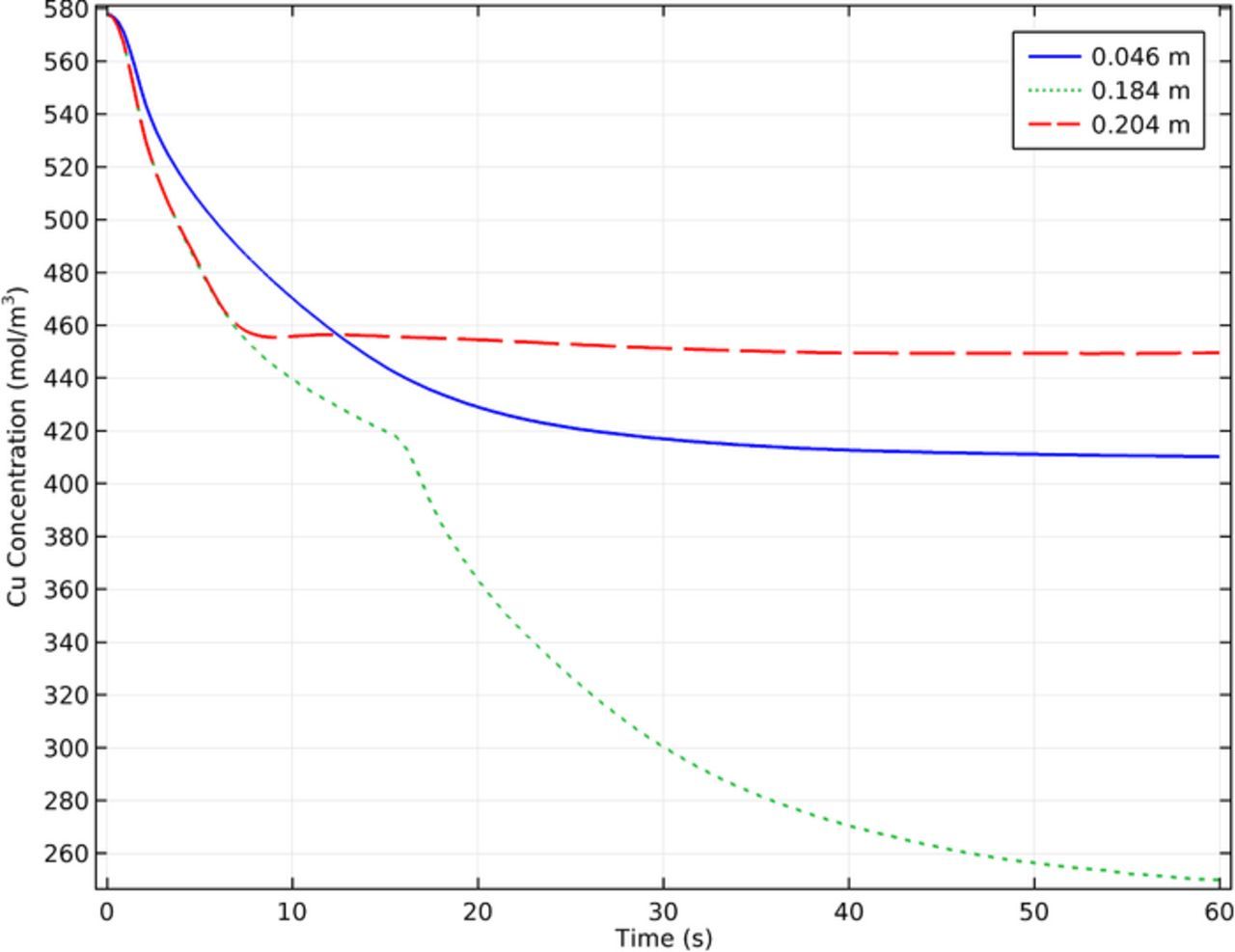
Figure 18 shows the boundary layer concentration gradient at a specific point on the cathode. This figure was included to provide insights into the nature of the cathodic boundary layer. Figure 18 shows the balance attempted in resolving the copper concentration in the boundary layer. In general the mesh was refined in areas of high gradients (such as the boundary layer).
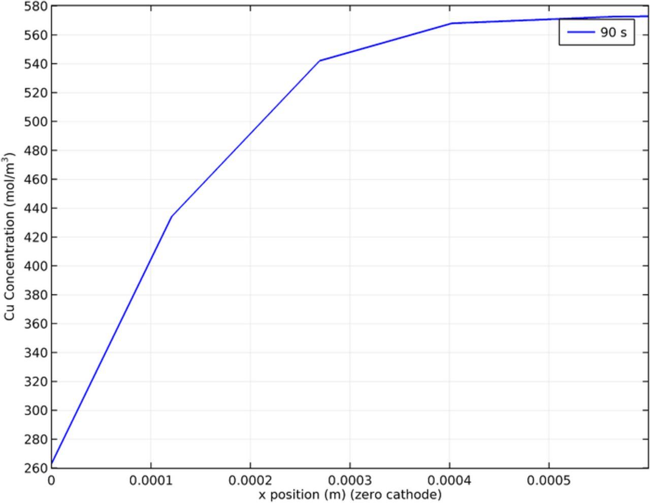
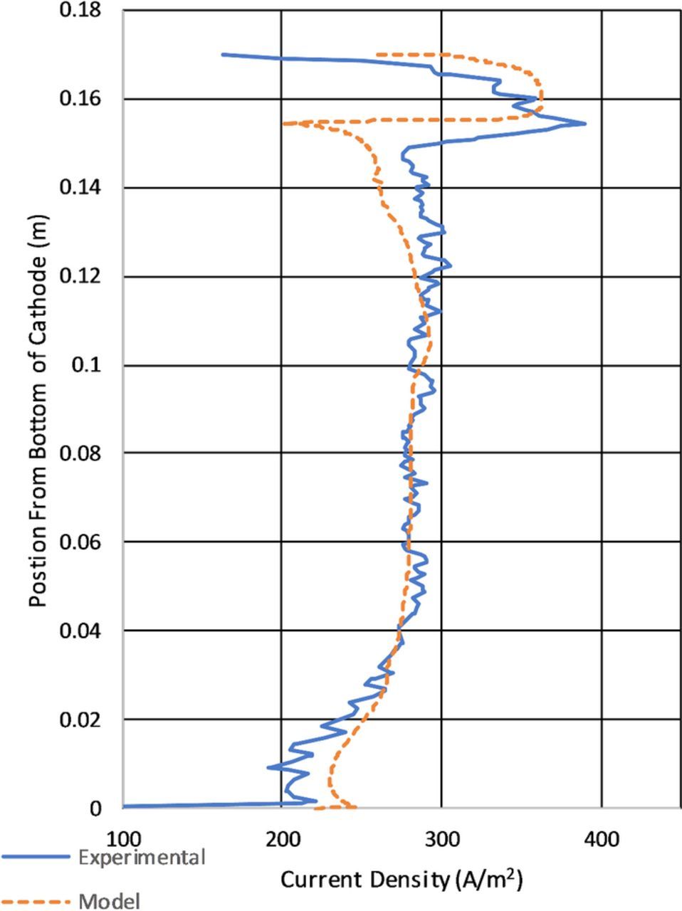
Figure 14 is the most significant figure type of the results section. It compares the average modeled current density at the cathode from 60–90s to the current density determined from deposit thickness. It also highlights the effect of the limiting of the electrode kinetics through overpotential. In general it appears that the measured current density and the model data are in general agreement. The largest apparent difference between the model calculated current density and that calculated from the deposit thickness is the apparent roughness. The current density variation shown in Figure 14 in the experimental data is due to two factors. The first is from the actual deposit roughness as shown in Figure 13. The second is due to the resolution of the 3D scanner used to measure the surface and discretize the measurements into a surface mesh for measurements. In the model apparent roughness in the results is likely due to numerical aberrations form the selected mesh size. Another important aspect to note in the apparent roughness difference of the data is the difference in the data types. The the copper deposit measured to determine the current density experimentally had time to fully develop roughness through the course of days. The model calculated current density was determined over 30s and without the benefit of mesh resolution and deposit/boundary layer feedback which did not produce the same roughness in the data. Observations of Figure 14 also show differences in the magnitude of the current density showing lower current densities in the area of the observed ridge and notch a the top of the cathode and overestimating at the bottom. The position of the feature at the top of the cathode shows reasonable positional agreement between the experimental and modeled results.
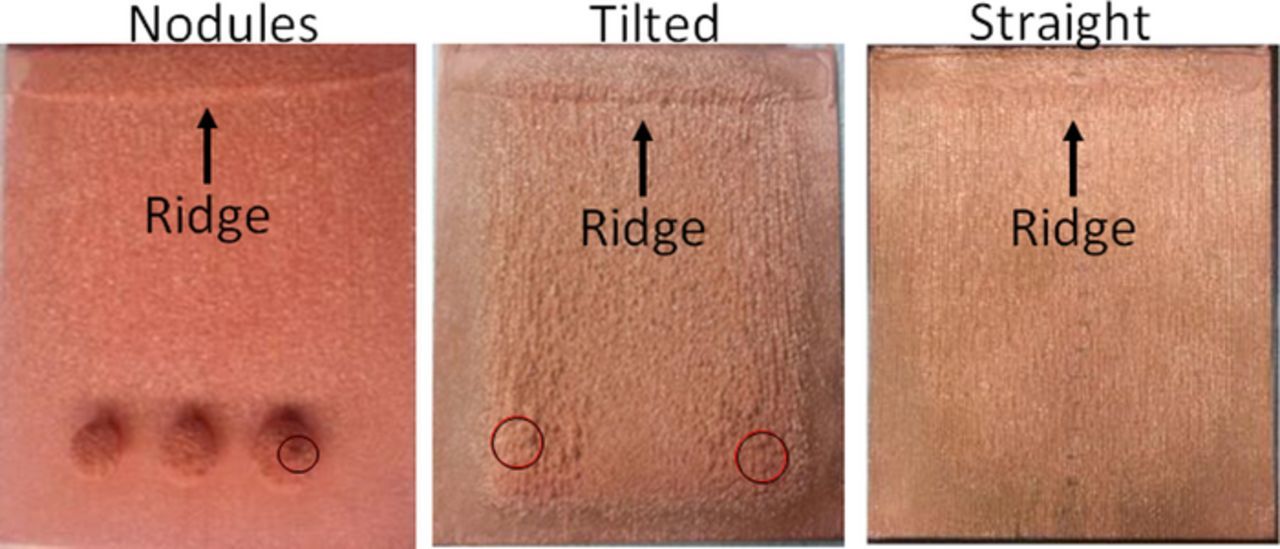
Figure 13. Experimental results showing a "Ridge" near the top of the cathode with circles indicating anodic contact.
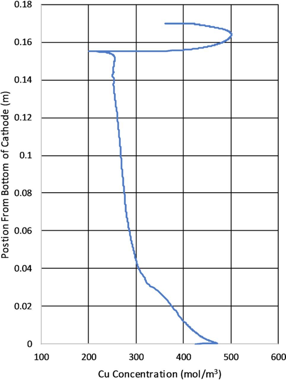
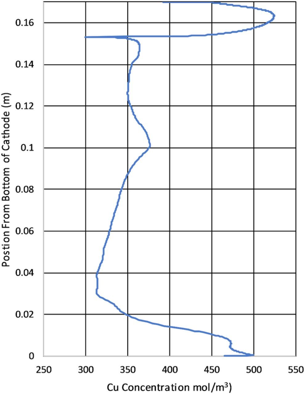
Figure 19 shows the copper concentration calculated from the model at the cathode surface at 90s. A key finding of the model is the higher copper concentration at the top of the cathode due to an increase in local mass transport. This along with the results in Figure 14 provide insights into the formation of a copper ridge at the top of the cathode. The results in Figure 19 are similar to those discussed in Figure 14. This is because copper concentration and current density are related by the Butler–Volmer expression. Note that in Figure 19 the results are presented without time averaging.
The extent of migration transporting the electroactive species of significant interest in eletrochemistry. Figure 20 shows the split between diffusive and migration fluxes as a ratio of the total flux. It this instance migration accounts for about 1/4 of the total flux. The model calculated results shown in Figure 20 are interesting in that across the length of the cathode the mode of transport as measured at the surface of the cathode varies by approximately 10%. As shown in Figure 20 the top of the cathode shows increased transport due to migration. This is explained by the higher copper concentration at the cathode in this region as shown in Figure 19. Thus with a higher concentration the concentration gradient is less owing to lower diffusion and increasing migration. The difference between migration and diffusion and the effect on transport will be covered further in future works where additional species composing the electrolyte will be considered.
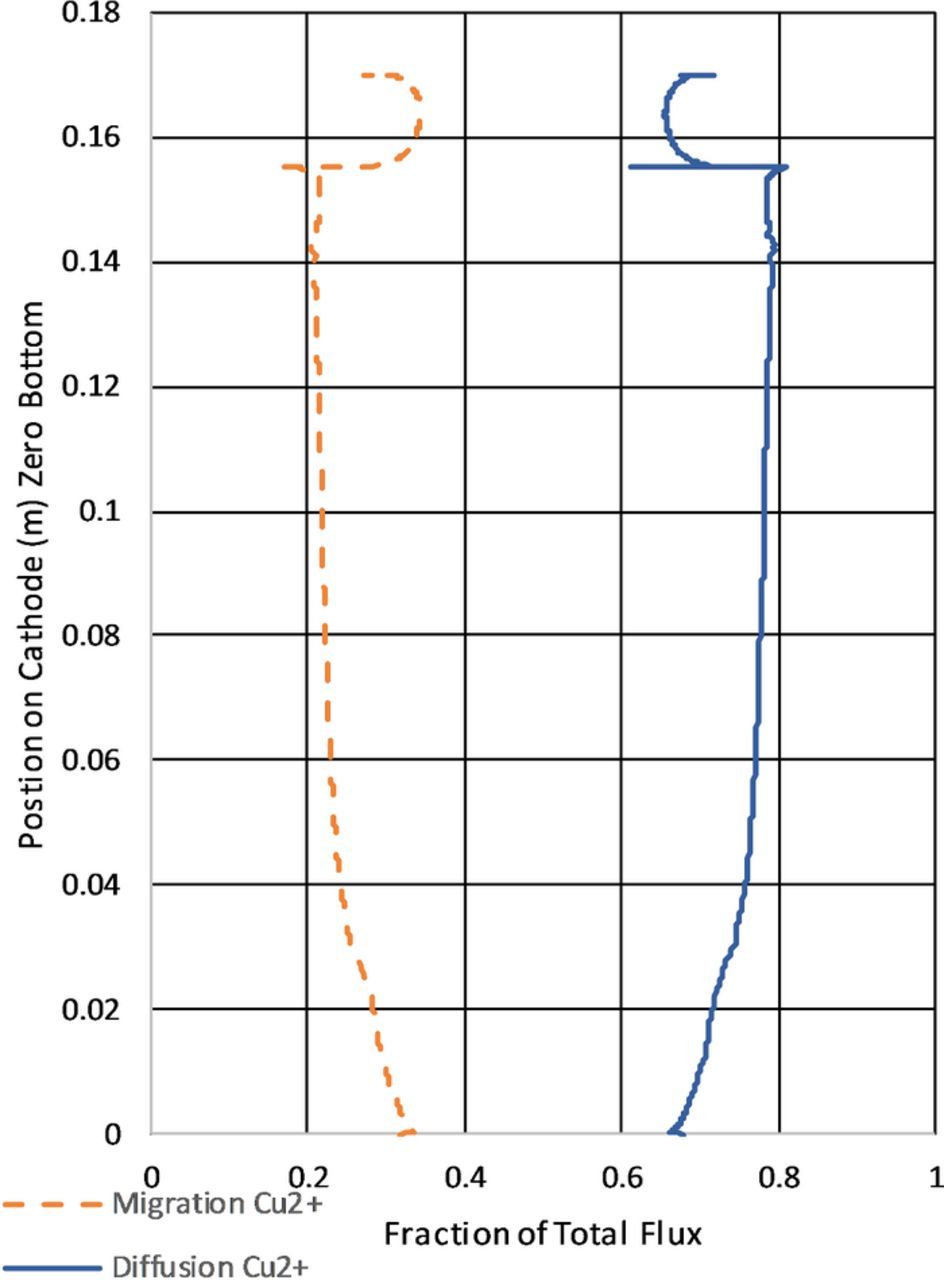
Figure 21 is similar to Figure 19 showing copper concentration but with the difference of presenting data in the cell rather than the cathode. In particular, Figure 21 shows concentration differences due to the transport form the electrolyte flow.
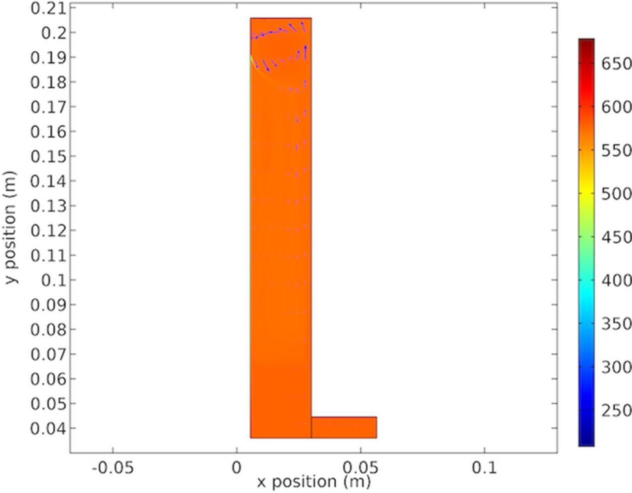
Figure 22 shows the electrolyte velocity showing the vortex formed at the top of the cell. This Figure shows the cause of the results in Figures 14 and 19. The results in Figure 22 are significant in showing the formation of a single stable vortex at the top of the cathode. This is due to the height of the cathode chosen. If the cathode was taller the vortex would become unstable and separate. This is the reason that the notch phenomenon is not observed in full size electrowinning cells.
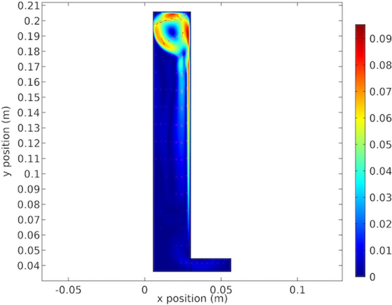
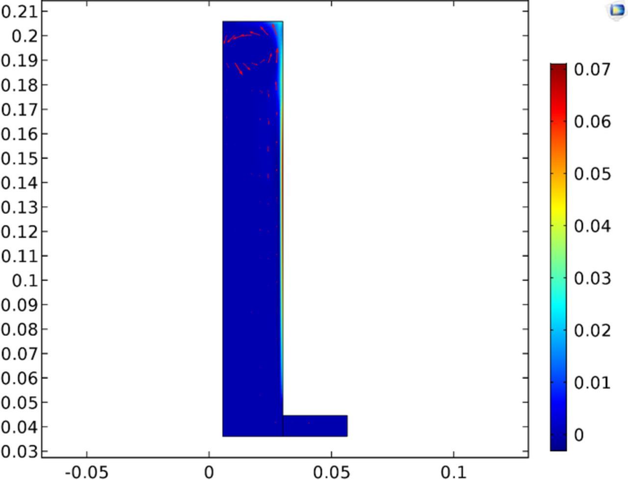
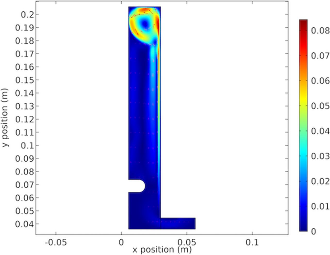
Figure 23 shows the gas fraction in the cell. The results show little carryover of the gas back down the cell, with the majority exiting the electrolyte at the top. The maximum gas fraction is listed at 0.007 and occurs in only a limited portion along the anode, with the majority of the cell below the 0.01 threshold for mentioned for the low gas assumption for the bubbly flow governing equations. This assumption was made in light of the higher local gas fraction due to the limited portion of the electrolyte having a higher gas fraction and the vindication of the results. It appears sufficient to maintain the low gas fraction simplification in light of adding additional computational expense.
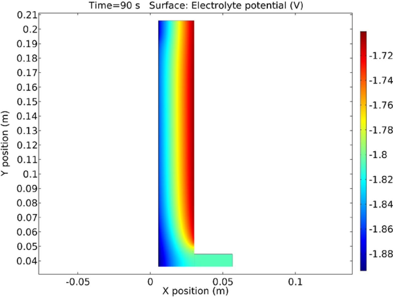
It is also beneficial to discuss the results in terms of cell and electrolyte potential. Figure 24 shows the cell potential at 90s during the simulation. The anode is considered zero potential. Thus the electrolyte at the anode is slightly under -1.72 Volts due to the equilibrium potential and over-voltage predicted by the electrode kinetics. Similarly, the cathodic equilibrium and over-voltage is calculated by the program to give an overall applied voltage. It is interesting to note the increased potential gradient at the top of the cell. Figure 20 shows the increase in copper flux due to migration at the same location from the increase in copper concentration in this area. This would also suggest a cause for the higher electrolyte potential gradient and lower electrode potential from the increased local current density. However, the reaction rate is moderated by competition from the increased surface concentration and the subsequent increase in over-voltage from the Buttler-Volmer equation. The cause of this feature is due to the influence to the electrolyte flow manifest in this region.
The mass transport coefficient is provided in Figure 25 calculated according to equation:
![Equation ([41])](https://content.cld.iop.org/journals/1945-7111/165/5/E190/revision1/d0041.gif)
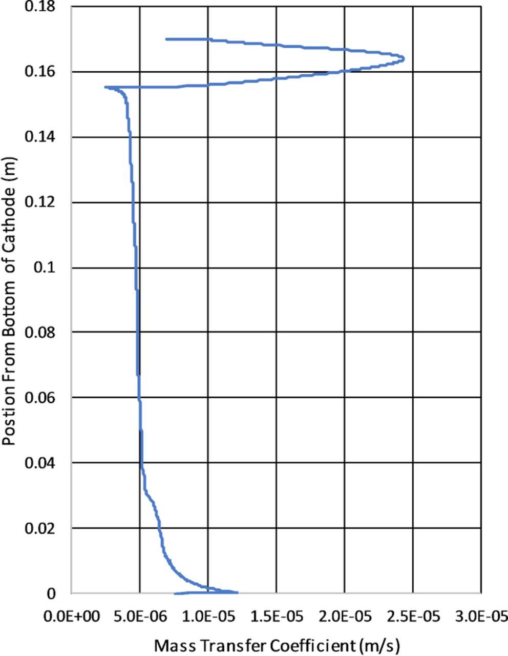
Figure 25 shows the variation of the mass transport along the cathode and includes the contributions from both migration and diffusion. From this plot it is apparent why there is enhanced deposition at the top of the cell with roughly 5x increase in mass transport at highest compared to the lowest transport areas. In the instance of electrowinning in the presented test cell the local transport variations are significant as shown by Figure 25 and should not be ignored.
Titled cathode results
The tilted cathode shows many of the same features as the straight cathode with primary difference being the current density distribution from the spacial alignment. Because of this the discussion in this section will focus primarily on the differences between the straight and tilted cathode.
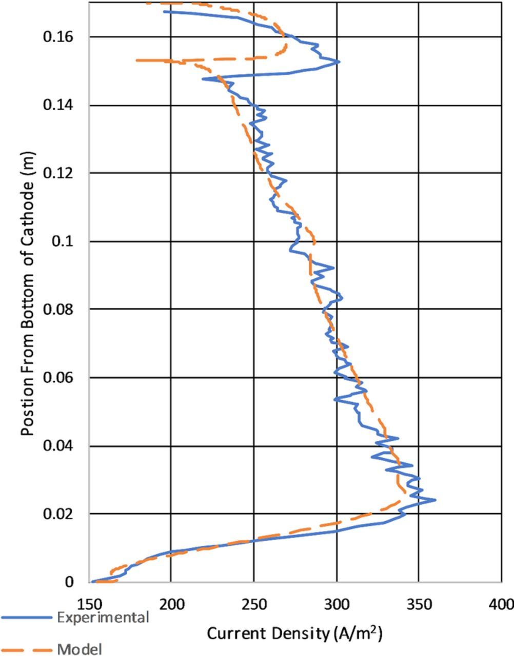
Figure 15 shows the current density comparison from the experimental to the model. It is helpful to contrast this to Figure 14 for the straight plate geometry. In comparison, the tilted cathode shoes a less pronounced ridge at the top of the cathode because of the lower local current density. The highest current density on the tilted cathode is located at the point closest to the anode at about 0.02 m from the bottom of the cathode. This is because of the lower potential drop in the electrolyte from the decreased distance to the anode. The current density is lowered somewhat by the electrode kinetics. The increase in current density showing a maximum at 0.025 is due to the proximity of the cathode to the bottom of the anode. This increase is explained by the lower electrolyte resistance caused by the decrease in distance. From Ohm's law the lower resistance will increase the current flow to this area. However, electrode kinetics cannot be discounted with current density also determined by local overpotential which has concentration dependence.
Figure 26 shows the copper concentration along the cathode for the tilted geometry. If varies significantly from Figure 19 showing the straight cathode in that the location of the titled cathode closest to the anode show lower copper concentration. This is because of the increased current density from the proximity to the anode. The results showing the lower concentration at the point of minimum anode to cathode separation distance is significant in terms of the moderating impact of overpotential and electrode kinetics due to concentration. As the concentration decreases the overpotential will need to increase negating some of the lower electrolyte resistance at the point of closest proximity.
In conjunction with Figure 26, Figure 27 shows copper concentration across the electrolyte domain. The apparent difference between the results in Figure 27 versus those of the straight cathode in Figure 21 are not great. The maximum velocities in each are approximately equal and the tilt in the lower part of the cell does not significantly vary the vortex at the top of the cell.
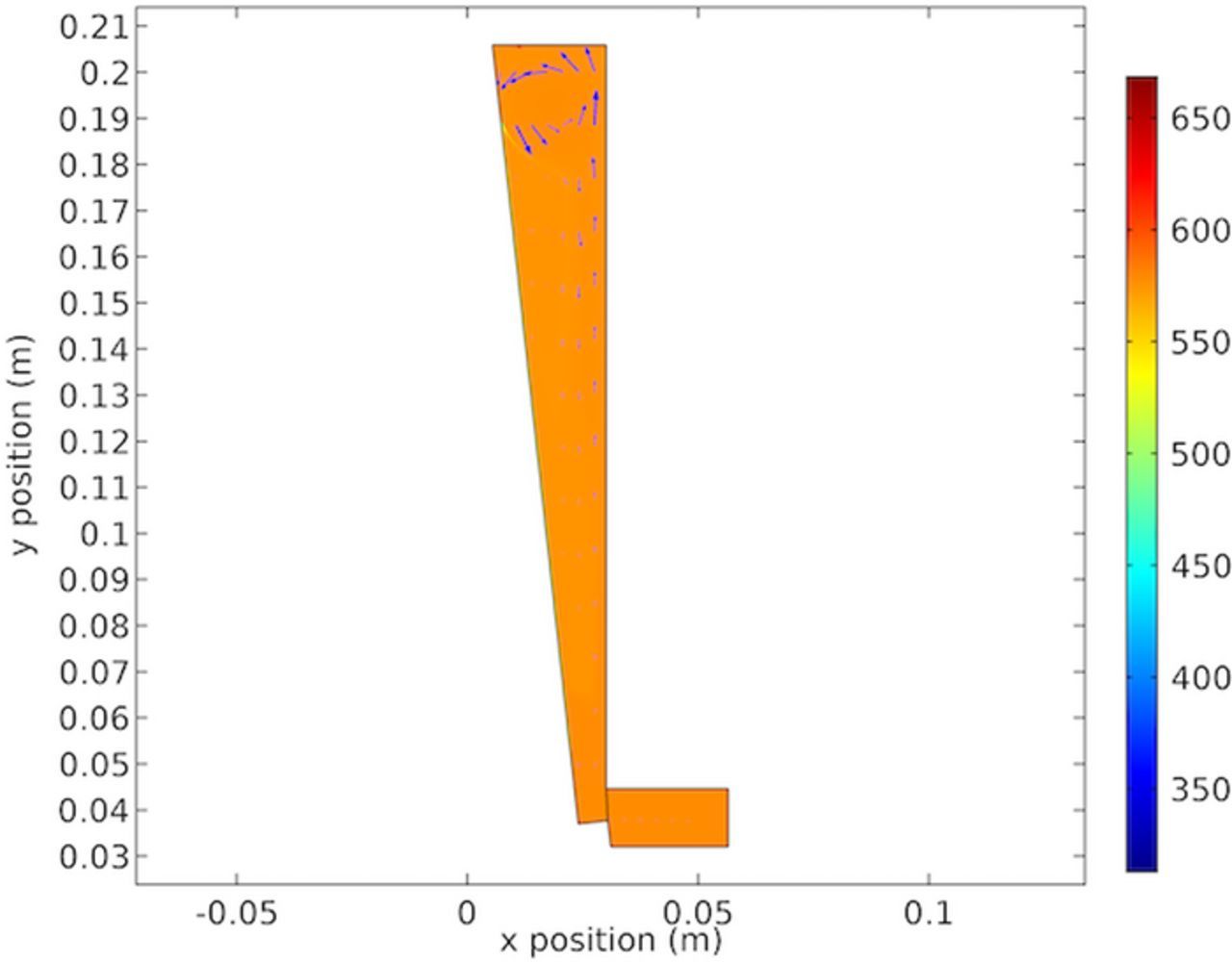
Figure 28 shows much the same velocity profile as does Figure 22. The geometry does not seem to affect the vortex at the top of the cell owing to similar dimensions at the top where recirculation occurs. The difference in ridge current density is due not to the mass transport, but rather to the current density distribution from proximity to the anode with associate drop in electrolyte resistance.
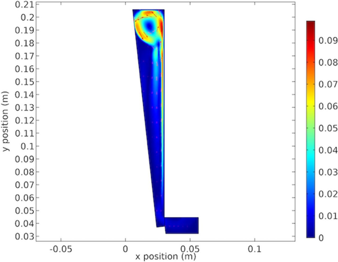
Figure 29 shows the gas fraction in the cell. Again, there is not much difference between the straight and titled geometries that is of significance.
Nodule cathode results
Out of all of the current density profiles the most difficult to obtain is the cathode nodule. A brief description of the process is warranted because of the difference in data presentation and collection methods. The process begins by obtaining a 3D surface scan of the deposit as shown in Figure 30. Figure 30 shows the nodule cathode scan with the base that it was scanned upon. The base is oriented to the x, y, z axes via translation and rotation. Thus the thickness of the cathode may be subtracted out. These data are then imported in to a CAD program (Solidworks) where a cut plane is utilized to obtain a 2D profile along the centerline of the cathode.
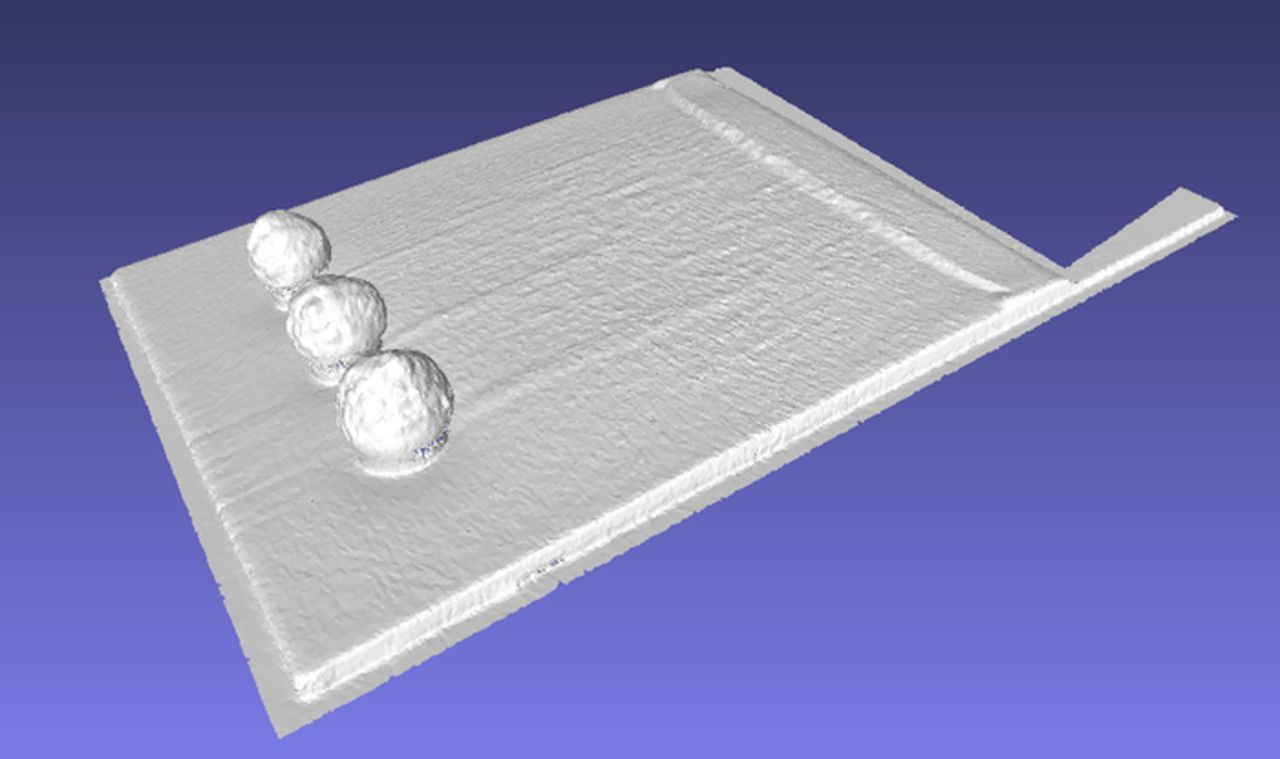
Figure 30. 3D scan showing nodules and base plane for geometric reference.
The cathodic nodule data are best presented in terms of perimeter or arc length along the cathode which allows presentation of the data in standard xy graphical form. The second discussion point is how the deposit profile was determined. Figure 31 shows the cross-section diagram of the nodule with electrodeposit. As with all of the presented data the cathodes were processed with a 3D scanner. Care was taken to scan the underside of the nodule deposit due to overhang. A centerline plane was used to determine the intersection profile for export for the calculation of current density. In the case of the nodule the deposit was superimposed over the original geometry as shown in Figure 31. A point was determined at the base of the nodule of theoretical "zero current". This is a simplification based on the normal vector of deposit growth. The lines on each side of this point indicate where current is fully dependent on deposit thickness. A series of measurement lines normal to the original surface were drawn to determine deposit thickness. Thus, deposit thickness and associated arc length were determined. This allows direct comparison of measured data to the model output.
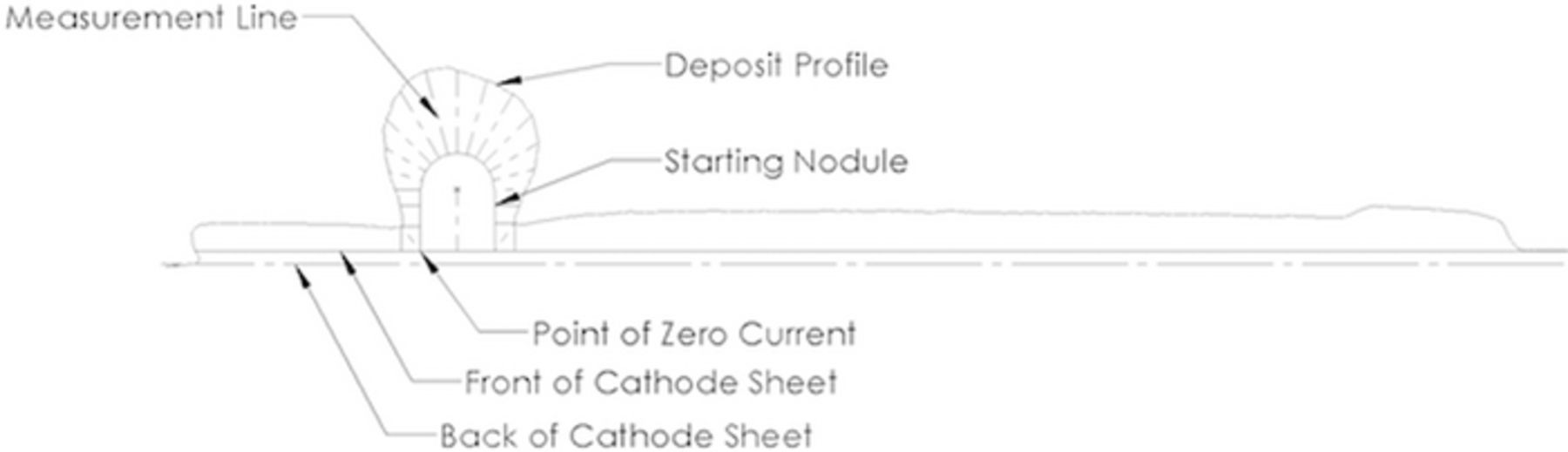
Figure 31. Cross section of nodule showing measurement lines for reference.
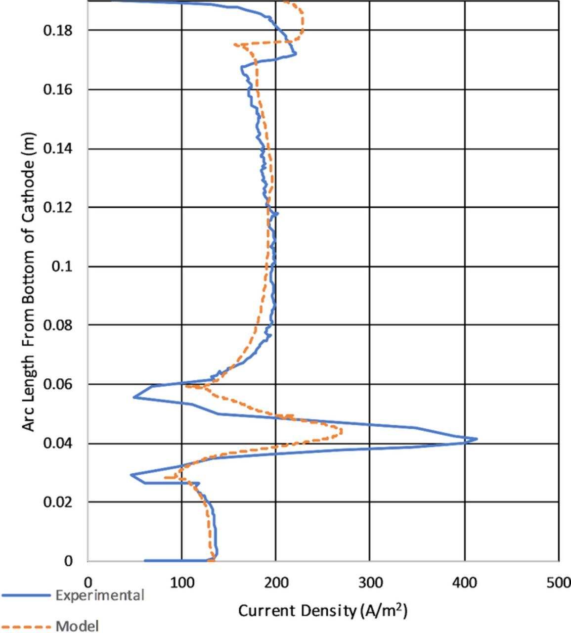
Figure 16 shows the comparison of current density from experimental to modeled. The model shows good agreement with the experimental, except at the nodule. The troughs at the nodule base are underestimated by the model. This may be due to the method of determining the current efficiency from the deposit thickness. The model did not have to contend with changing boundary geometry. Also, the maximum current density is under represented by approximately 130 A/m2. This may be due to the additional nodules shown in Figure 30. These were included to test different shapes and in the instance of this model the geometry for the middle nodule was utilized. However, this should have been compensated by the determination of the average current density from the deposit thickness. Because numerical integration was used to determine the nodule deposit thickness, the center average between adjacent data points was used. That is why in Figure 16 the current does not reach zero at the nodule base.
Figure 32 shows the copper concentration at the modeled cathode surface. The variation is quite pronounced particularly along the nodule where the mass transport varies widely. It is important to consider that the 2D representation considers this feature as infinitely wide and the flow around the nodule sides is not considered.
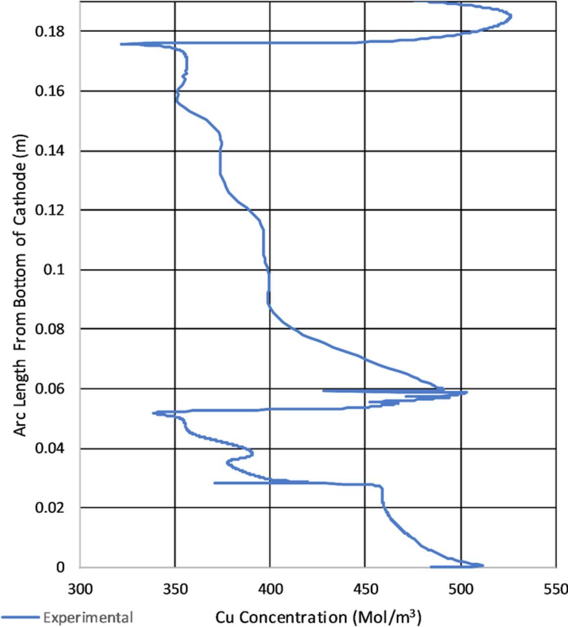
Figure 33 shows the copper concentration in the cell. Note the concentrations due to the flow effects from the nodule and the resulting boundary layer. Of all the three geometries presented the nodule cathode shows the most variation along the cathode. In Figure 33 and Figure 32 the coupled electrolyte resistance decreased due to anode proximity and fluid flow contributions lead to the variation in the copper concentration.
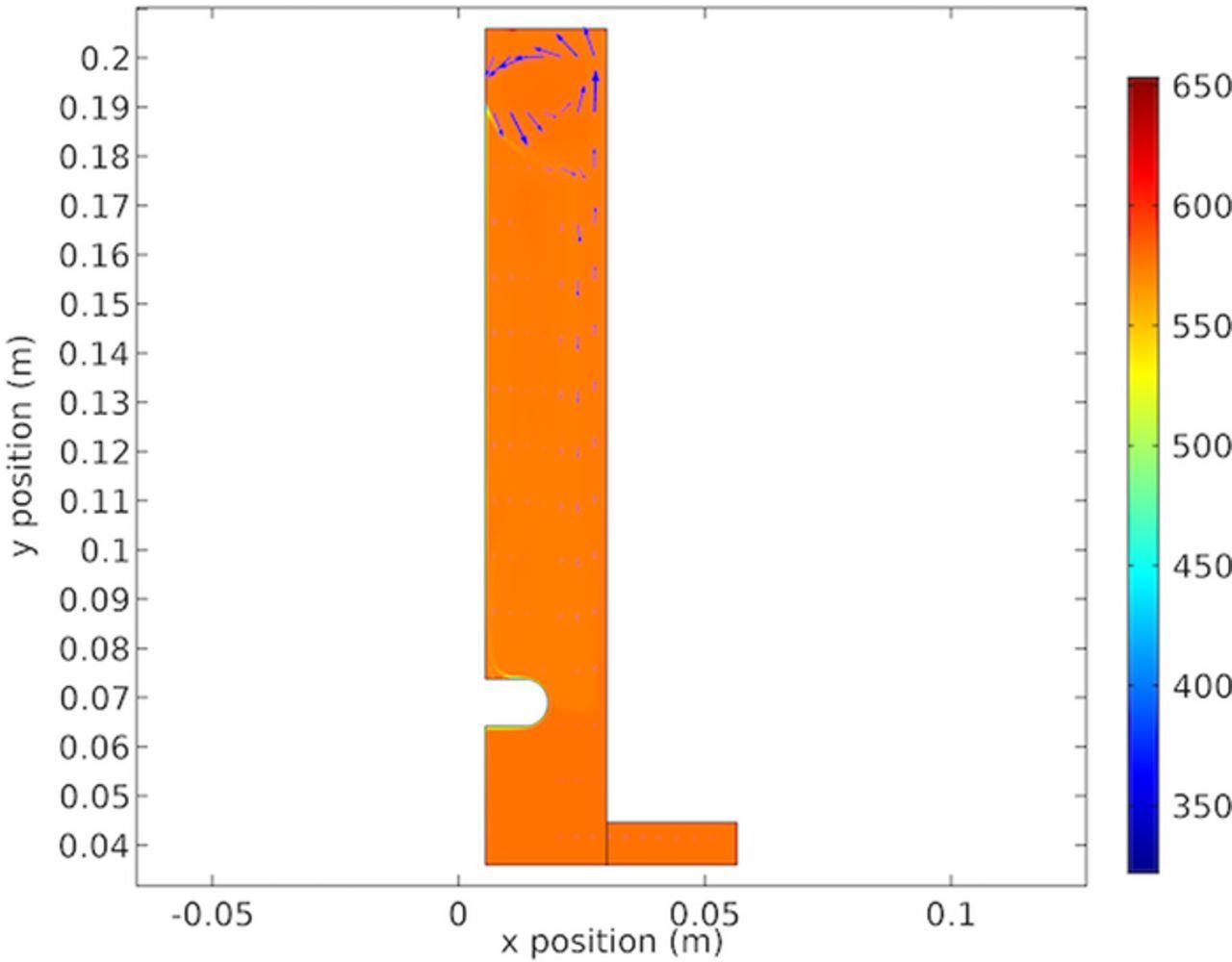
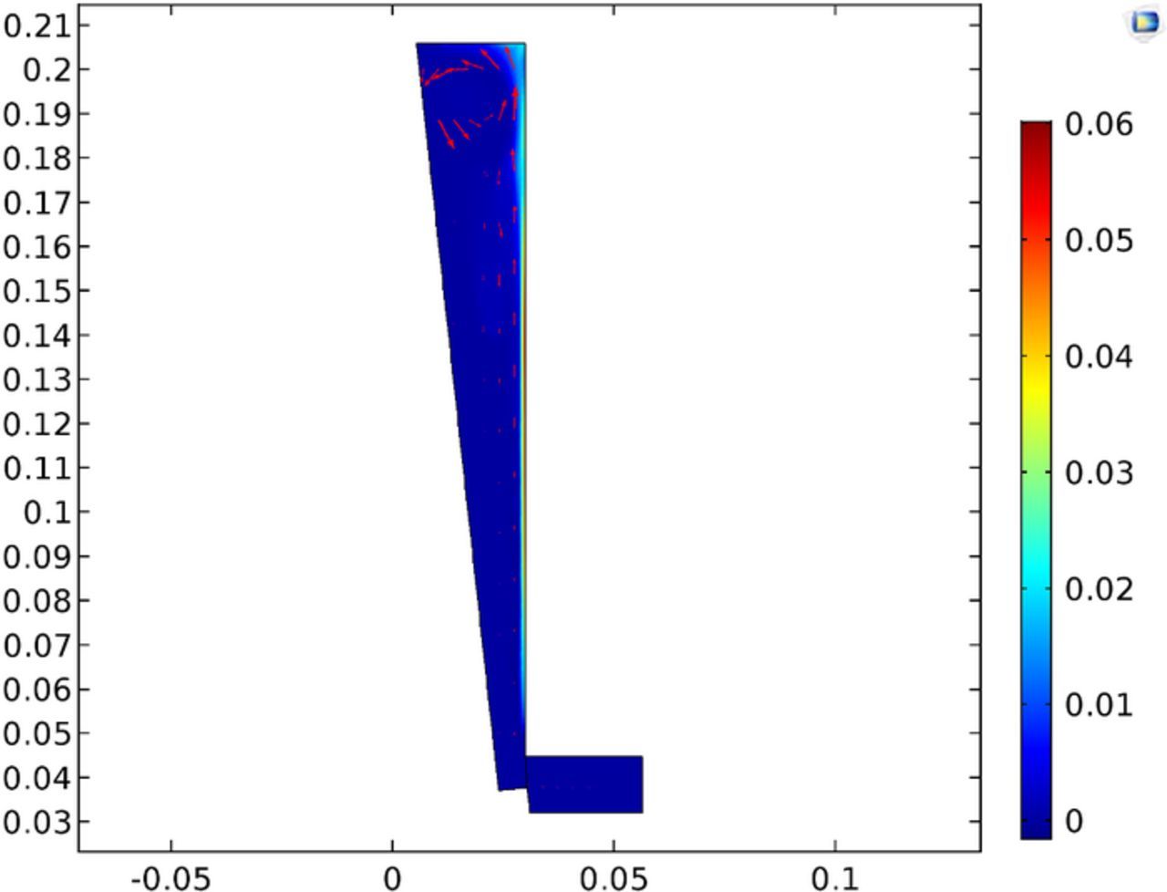
Figure 34 shows the electrolyte velocity which explains the mass transport effects in the cell. Compared to the straight cathode in Figure 22 the nodule cathode in Figure 34 shows a slight decrease in maximum fluid velocity, but largely remains the same as the straight cathode. This difference is the result of the lower modeled current density as shown in Table VII.
Lastly, Figure 35 shows the local gas fraction in the cell. Of note is the lower gas fraction presented by this model. This can be explained by Table VII with a lower current density being utilized.
Discussion of flow conditions
Figure 13 shows the results of completed experiments. The formation of a ridge near the top of the cathode is common among them.
To our knowledge this ridge has not previously been noted extensively or discussed in detail. Larger industrial cells do not have this ridge. Results shown in Figures 22, 28 and 34 show the fluid circulation vortex at the top of the cell. This affects the cathodic copper concentration shown in Figures 19, 32 and 26. Further, because of the decrease of copper along the cathode, the electrolyte becomes less dense and rises buoyantly. This upward flow of lower concentration electrolyte meets the vortex at the top. This is seen in the lower concentration "ribbon" shown at the top of the cell. The increased mass transport at the cathode top is due to flow. This further increases the local current density as shown in Figures 21, 27 and 33. These conditions create the ridge in the deposit near the top. This effect is shown in the cell velocity plots in Figures 22, 28 and 34. The selected height of the cell was serendipitous. Shorter cells would reduce the vortex and taller cells have multiple unstable and random voracities that eliminate the ridge. Thus, in our study the model and measured validation of the ridge formation provide confidence in the accuracy of the model.
In this model the calculated Reynolds number is above 10,000. This was shown in the model convergence in that the fluid flow is predominantly laminar with a slight wobble. This flow regime is problematic in terms of computing. As such the model was run to 60s which allowed for fully developed flow. The following 30 (60–90s) seconds were used to determine the average current density provided.
Concerns and potential issues
In reviewing this work there are a number of potential issues that should be addressed.
The first utilizes three species for electrochemical modeling. Cu-Acid systems are known to have multiple species which are not represented. As the Nernst–Planck equations are solved these will have an effect on the system such as changing the resistivity, cell potential and limiting current density due to supporting electrolyte. It is intended that this will be investigated in future work with this paper serving as a preliminary investigation.
The second is with regard to the position of the inlet. Due to the 2D simplified geometry there is not sufficient mixing in the cell to draw electrolyte from the bottom of tank. So, by necessity electrolyte must flow between the electrodes. To address the short run times utilized in the model on bulk concentration, the steady-state cell copper concentration was determined and utilized. Due to the small inlet velocity, the modeled fluid velocity between the electrodes is not expected to be affected significantly.
The third point is that the model utilizes a 2D representation of 3D flow effects. Observed flow conditions show that the bubbles induce a flow that moves the electrolyte at the top of the cell both down and out to the sides. This increases the mixing and may be the reason for the vertical difference of the ridge on the top of the cell when compared to experimental data. This is also compounded by the use of an average current density rather than the total cell current. These two issues would be better understood by a 3D model which may be pursued in subsequent work.
In conjunction with the third point, the fourth point is the lack of determination of the effects of the fluid structure interactions on the deposit shape. Ideally the model would be recomputed to allow for topological influences on the fluid flow. This will be examined further. Also, there are some errors due to scanning resolution and needed mesh preparation for deposit measurements.
Lastly, another concern of this model is the lack of the inclusion of a turbulence model, particularly in light of the works of Leahy et al.5,7 Also anther concern will be the treatment of bubbles, particularly in areas of where the local gas fraction exceeds that of the low gas concentration simplification. The Hadamard–Rybczynski for un-interacting bubbles is utilized where there is likely bubble interactions. We feel justified mentioning these shortcomings in view of the results with the following explanation. The purpose of this work is to better understand cathodic deposition processes. As such fine meshes on cathode were utilized in an attempt to adequately resolve the boundary layer. Thus the anodic boundary mesh was set as course as practical to provide the minimum resolution necessary for the bubbles to be modeled and provide buoyancy force to the electrolyte. Although not as rigorous as other approaches mentioned, this allowed computational time to be improved so as to allow utilization of the Nernst–Planck equations for transport. For this reason experimental validation was critical to justify such approaches and show model performance.
Conclusions
Overall the experimental results of the straight and tilted cathodes align well with the 3 species model presented. The nodule cathode experiment appeared to under predict the current density on the cathode. Euler–Eluer flow with the appropriate Nernst–Planck coupling for transport modeling appears to be well suited for this application. It is interesting the alignment is in general agreement with a substantial deposit thickness. However, additional work is needed to further investigate the effects of fluid structure interactions, speciation and current efficiency.
Acknowledgments
The authors gratefully acknowledge the AMIRA organization which supported this work with grant P705C. In addition, Joshua Werner gratefully acknowledges the SME foundation Ph.D. Fellowship grant which supported him during this work. Jae-Hun Cho and Steve Evans are also recognized for their contributions in the experimental sections of this work.
ORCID
J. M. Werner 0000-0002-9025-2986