Review—On the Application of the Scanning Vibrating Electrode Technique (SVET) to Corrosion Research

A. C. Bastos; M. C. Quevedo; O. V. Karavai; M. G. S. Ferreira

doi:10.1149/2.0431714jes

The Scanning Vibrating Electrode Technique (SVET) has been applied to corrosion research for about three decades but its use remains restricted to a few groups around the world and the application in corrosion and electrochemistry is still far from its full potential. The technique was originally developed by biologists in the decades of 1960–1980^1–4 to measure ionic currents involved in cellular differentiation,⁵ morphogenesis,^6–8 tissue regeneration^9–12 and electrophysiology,^2,13–15 areas where it is known as Vibrating Probe. The application to corrosion studies started with Isaacs in the 1980s.^16–19 Until then the potential distribution in solution was measured with reference electrodes, sometimes with Luggin-Haber capillaries, following an original idea of Thornhill and Evans^20,21 and Agar and Evans.^22,23 The concept was continued by several authors, notably Copson, Jaenicke, Akimov and Rosenfeld.^24–32 The book of Kaesche includes a chapter where most of these studies are analyzed.³³ In 1981, Isaacs and Vyas made a review of papers using this experimental approach and introduced the acronym SRET (Scanning Reference Electrode Technique) to designate the group of mapping techniques based on non-vibrating reference electrodes.³⁴ Curiously, SRET is now emerging in the field of imaging electrochemistry under the name of scanning ohmic microscopy.^35–37 SRET and SVET have been used to study galvanic corrosion,^38–42 pitting corrosion,^31,43–46 crevice corrosion,⁴⁷ stress corrosion cracking,⁴⁸ microbiologically influenced corrosion,^49–51 inorganic coatings,^52–55 painted metals,^56–60 corrosion inhibitors,^46,61–66 corrosion of weldments^67–70 and conducting polymers.^71,72 This list is far from complete. The references were selected because either they are the first study using SVET in each of these applications or they show significant and representative examples of the SVET capabilities. This work does not provide an exhaustive review of studies using SVET, rather it intends to be an introduction to the technique with examples from the authors. The interested reader will find reviews of published work using SVET and SRET elsewhere.^73–77

Operating Principle

Possibly the best way to understand how SRET and SVET work is to consider an electrochemical cell with parallel electrodes like the one depicted in Fig. 1a, where a current of 100 μA is flowing. The cross section area of the cell is 1.50 cm² giving a current density of 66.7 μA cm⁻². Fig. 1b shows the potential difference measured at selected points of the circuit, including the ohmic drop in solution, which is high in diluted solutions (low conductivity, high resistivity) and almost negligible in concentrated solutions. The ohmic drop profile was measured with a reference microelectrode that was moved with respect to another reference electrode kept in a fixed position – Fig. 1c. The electrical field in solution was about 120 mV cm⁻¹ in 0.005 M NaCl and 1.5 mV cm⁻¹ in a 100 times more concentrated (and 78 times more conductive) medium. The current density in solution, i, can be calculated using

which is a form of Ohm's law, where κ is the solution conductivity, E is the electric field in solution and ΔV is the potential difference between two points separated by the distance Δr in the direction of current flow. Fig. 2a presents the current density calculated by Equation 1 using the data in Fig. 1c and Δr = 20 μm (details in the Supplementary Material). Significant scattering is observed in 0.5 M NaCl but the average value is similar in the two solutions and close to the theoretical value of 66.7 μA cm⁻².

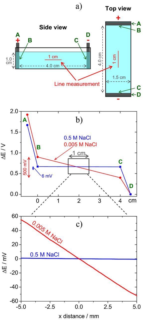
**Figure 1.** a) Sketch of the electrochemical cell with parallel graphite electrodes, b) potential profile in the cell measured in points A, B, C and D when passing a current of 100 μA, c) ohmic drop measured with a scanning reference microelectrode in a line at the center of the cell (Experimental details in Supplementary Material).

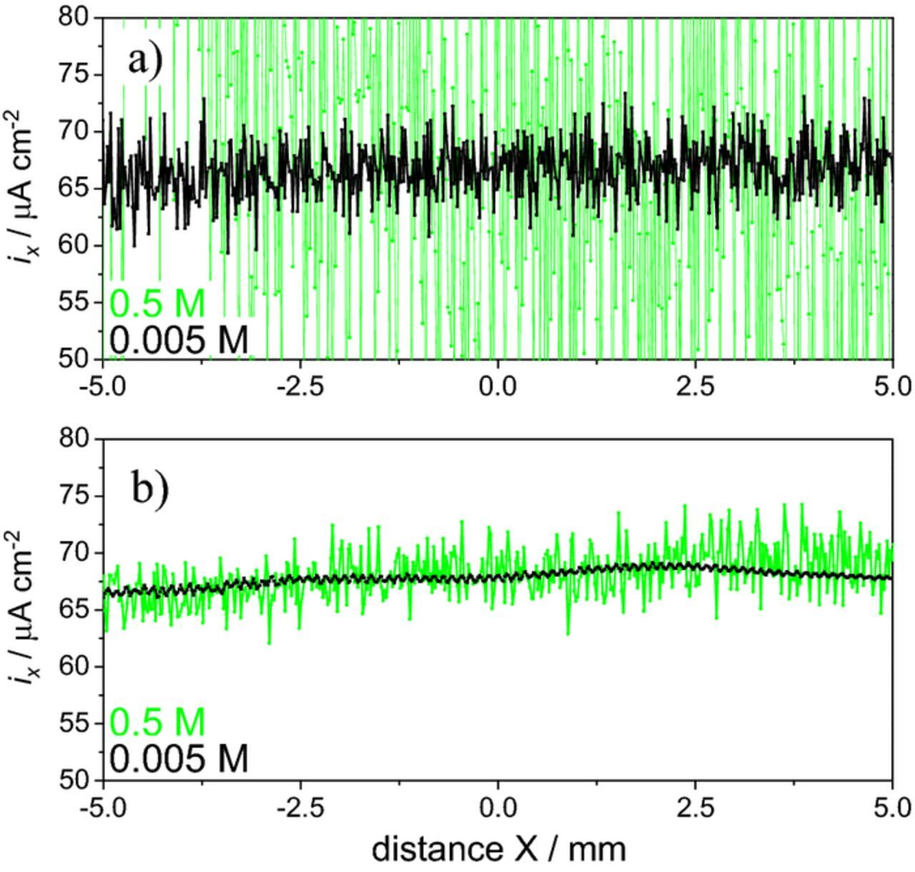
**Figure 2.** Local current density, a) calculated from SRET data and b) measured by SVET. (Experimental details in Supplementary Material).

What has just been described is an example of an SRET measurement. A variant of this technique employs two reference electrodes with micro Luggin-Haber capillaries³⁰ (pseudo-reference electrodes of silver, gold or platinum are also used) with fixed distance between them and Δr in the range of 10 μm to 1 cm. The two electrodes move together while scanning the sample and the potential difference between them is readily obtained. A different design was developed to study cylindrical specimens.^78–80

The current density obtained by SRET is prone to noise, a problem that intensifies with increasing solution conductivity. The noise can be significantly reduced and the sensitivity increased by making the electrode vibrate. The vibration creates a signal modulation (sinusoidal signal) that is used by a lock-in amplifier to substantially increase the signal-to-noise ratio.^2,4 This is the basis of the SVET and the main difference compared to SRET. Both techniques give ionic current densities from measurements of the potential in solution. Fig. 2b shows the current measured by SVET in the same conditions used for Fig. 2a where it is possible to observe values close to the theoretical one but with significant noise reduction. The main advantage of SVET is thus the high signal-to-noise ratio.

Calibration

In practice, the relation between the potential measured by SVET and the current density associated to it is obtained by calibration. There are different ways of performing the calibration, depending on the system.^2,4,9,81 What is now described is the typical procedure for the instrument produced by Applicable Electronics LLC (AE),⁸² which is the one used by the authors. The SVET probe is placed at a given distance (usually 150 μm) from a point current source that drives a known current I (normally 60 nA). The point source can be an insulated metallic wire with an electroactive tip of 3 μm diameter or, alternatively, a glass micropipette with 2 μm diameter tip, filled with the testing solution and a platinized platinum wire inside as current source. The current density i at a distance r from the point source is given by,^2,83

where (4 π r²) is the area of the sphere with radius r. Fig. 3a shows a representation of the current lines flowing away from the point source and spherical equipotential surfaces centered on the point source. For each sphere or radius r, I is always the same and the current density is obtained dividing the total current by the area of the sphere. Fig. 3b plots the variation of the current density, i, with the distance to the source, r, for I = 60 nA. The relationship between i and r is linear in a log-log plot, as shown in Fig. 3c. For the typical calibration, the current density measured at the calibration point is i = (60.0 × 10⁻⁹ A) / [4 π (150 × 10⁻⁶ m)²] = 0.212 A m⁻² = 21.2 μA cm⁻². The SVET from AE measures the current density in two orthogonal directions (X and Z) therefore the calibration is performed in two points, one for each vibration. More details can be found in the literature.⁴

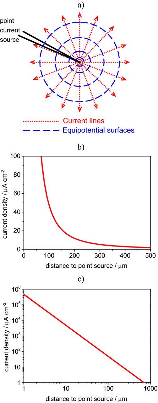
**Figure 3.** a) Representation of the current lines flowing from a point source (glass capillary with platinum wire electrode inside), b) variation of the current density with distance from the point source (for I = 60 nA) calculated by Equation 2 and plotted in linear scale and c) the same plot in log-log scale.

The potential measured by SVET in any point is related to the local current density i by

which is Equation 1 written for the potential difference and ρ is the solution resistivity. During the calibration, the system measures the local potential difference and, knowing the theoretical current density at the calibration point, the proportionality factor between ΔV and i is determined. Then, during the measurements the proportionality factor allows one to relate the potential difference measured between the ends of the vibration with the current density that is flowing in the point of measurement. The calibration remains valid in different media provided the correct conductivity is updated when changing solution or temperature. If the conductivity changes in the course of a measurement, deviations from the true current density will appear. Other factors that influence the proportionality factor, like system gain, frequency and amplitude of vibration are usually selected when the system is installed and not altered thereafter. Changing them requires re-calibration. It is important to note that the 'point source' calibration cell involves precise knowledge of the SVET probe tip relative to the point source electrode. Moreover, if instead of a wire inside a glass capillary, the current source is a metallic tip in low electrolyte concentration, local pH change arising from water electrolysis at the point source can significantly alter the local solution conductivity leading to calibration error. An alternative 'tube cell' calibration has been described which avoids these difficulties.⁸¹

In the cell shown in Fig. 1 the current density is the same everywhere in the bulk of the solution and so is the electric field sensed by SVET. Fig. 4 presents maps of the current density measured in 3 orthogonal planes in the middle of the electrochemical cell. For each plane, maps of the current density detected by the probe X and Z vibrations (respectively parallel and normal to the current direction) are presented. The maps from the vibration aligned with the current flux (X vibration) should show constant current density close to the theoretical value of 66.7 μA cm⁻². The maps from the Z vibration should present null current density. Small deviations from the expected values are observed which seem to reflect a small misalignment of the scanning planes with respect to the current path between the parallel electrodes. Sometimes larger local deviations were observed (e.g. maps YZ) indicating that even in simple systems with constant current, the measured values can have fluctuations most probably due to the electronics of the current source or in the measuring circuit.

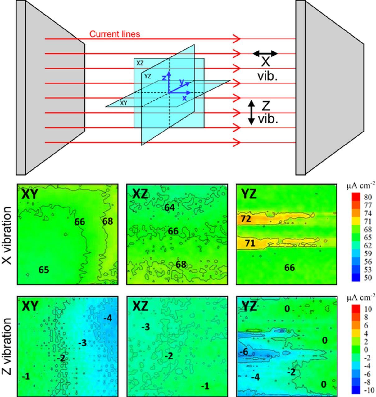
**Figure 4.** Maps of current density measured by SVET in the middle of the cell in Fig. 1 for a current of 100 μA and a theoretical current density of 66.7 μA cm⁻². Maps depict the current measured by the two SVET vibrations (x and z) in the three planes XY, XZ and YZ. The size of each map is 2 × 2 mm². (Experimental details in Supplementary Material).

Examples of Use in Corrosion

Mild steel in 0.05 M NaCl

In the cell of Fig. 1, anode and cathode face each other. In corrosion they are often side by side, on the same surface, with the current entering and leaving solution in different locations. A simple example is the corrosion of mild steel in near neutral sodium chloride solution. Fig. 5. shows images of the sample and SVET maps acquired at selected moments during the first 24 hours of immersion. The maps shown only the Z component of the current density, i.e., the flux normal to the surface. Green areas correspond to zero net current in the Z direction. Red areas indicate positive (anodic) currents which are related to the iron oxidation,

and blue is for the negative (cathodic) currents associated with the reduction of dissolved O₂,

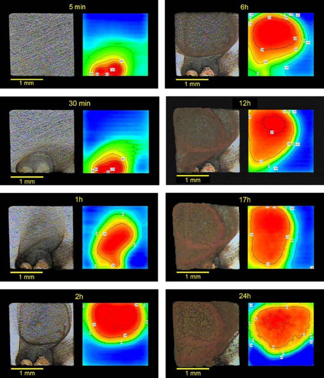
**Figure 5.** Stages of corrosion of a mild steel during the first 24 hours of immersion in 0.05 M NaCl. Values are current density in μA cm⁻². Blue color means negative (cathodic) currents and red means positive (anodic) currents.

Considering the conventional current direction, the positive current enters solution at the anodes and leaves at the cathodes. All ions in solution transport the current, anions (OH⁻ and Cl⁻) toward the anode and cations (Fe²⁺ and Na⁺) toward the cathode. These maps of the current density normal to the surface are the most usual in corrosion research. The main reason is that this is sufficient to describe the corrosion process by showing the position and magnitudes of anodic and cathodic sites over time. The information from the X vibration can be a complement especially if a more quantitative analysis is desired.

Fig. 5 shows that five minutes after immersion the optical image reveals an intact surface, while SVET already detects the currents whose consequences will be visible only in the image acquired after 30 minutes. SVET senses the activity before it is recognized by the naked eye or with a magnifying lens. The figure is a good example of the benefits of combining optical images and SVET maps. The optical pictures give the accumulated corrosion up to the moment they are acquired and do not differentiate the regions that are active then. In turn, SVET shows the "instant" activity, that is, the activity actually taking place during the time of map acquisition (5 to 30 minutes are typical), identifying the anodic and cathodic regions and providing a quantitative measure of the respective magnitudes. SVET can be considered a technique to image corrosion. It should always be used together with the optical images of the sample.

Galvanized steel

Steel sheet is often coated with a zinc layer to increase its corrosion resistance. When the steel substrate becomes exposed, it remains protected due to the galvanic action of the less noble zinc layer. SVET can be used to reveal the corrosion pattern of such a layered system. Fig. 6 shows a sample of electrogalvanized steel after 24 hours of immersion in 0.05 M NaCl together with various ways of presenting the same SVET results. The corrosion of the zinc layer occurred in a localized manner with steel being exposed in some points of the surface where the zinc dissolution was deep enough. Then the zinc oxidation continues in the border of those circular regions which enlarge as zinc corrodes. It is possible to present the current density in the form of 2D vectors, as in Figs. 6b and 6c. The arrows can be superimposed to the image of the surface giving a good imaging of the current flow. Alternatively, the current from the Z vibration suffices to identify the active anodic and cathodic regions and corresponding magnitudes – Figs. 6d–6h. In this example the anodic regions seem to coincide with the exposed steel but it is the zinc on its border that is oxidizing. The high anodic current magnitude masks the smaller cathodic current at the steel area. A few days are necessary until the steel area is large enough for its cathodic activity to be detected. Otherwise, the measurement could have been made closer to the surface to separate both currents.

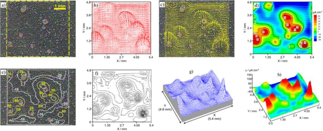
**Figure 6.** a) Electrogalvanized steel after 24 hours in 0.05 M NaCl and different ways of presenting the same SVET results: b) map of 2D current density vectors, c) map of vectors superimposed to the surface image, d-h) maps with the current density normal to the sample surface (from Z vibration). (Experimental details in Supplementary Material).

The majority of the maps in this paper were made with Quikgrid, a powerful, yet small (∼500 Kb) and free, software.⁸⁴ Many choices of presenting SVET data are possible depending on the objective of the study and the preference of authors. Mandatory should be the inclusion of the image of the sample surface with the indication of the mapped area together with the SVET map.

Cut-edge corrosion of galvanized steel

The corrosion of galvanized steel sheet frequently starts at the cut edges because this material must be cut before use. The cut edge is an area where the steel substrate and zinc coating are exposed and the sacrificial protection conferred by the zinc may be of short duration due to the poor anode to cathode surface area ratio (1/100). Even if an organic coating is applied on the sheet surface it does not offer any barrier protection in the cut edge. The initial stages of corrosion may involve anodic undermining of the organic coating followed by the formation of blisters near the cut edge. This is the weakest point from where corrosion starts. For this reason the corrosion of cut edges of galvanized steel has been extensively studied with industrial and model samples.^39,85-98 One of the studies using SVET described in the literature is presented in Fig. 7.⁹³ The sample is a cross section of hot dip galvanized steel (HDG) – 5000 μm low alloy carbon steel sheet with 40 μm zinc layer – embedded in epoxy resin and polished with SiC paper up to the grade 4000 and then with diamond solution up to the grade 1 μm. The careful polishing procedure allowed for homogeneous dissolution of the zinc coating. Because of this, SVET measurements in transversal lines were enough to describe with confidence the corrosion processes on the sample. After a few minutes of immersion in 0.03 M NaCl, a distinct pattern was observed on the steel, divided in two zones: a zone covered by visible white precipitated corrosion products which appear to have simply deposited on the surface, probably due to precipitation in the bulk solution (Area I), and an almost uncovered zone (Area II). The distribution of the normal component of the current density, J_y, measured after 40 min of immersion and 50 μm above the surface is presented in Fig. 7b. Three distinct regions were revealed: an anode localized over the zinc surface, a region of "zero-current" ("passive" zone) and a cathodic area on the opposite side of the steel. The interface between the "passive" and the cathodic zones correlates with the line of thick precipitates on the steel surface. The "passive" behavior was attributed to a self-healing mechanism by the formation of an oxide film during the very early stages of the immersion when the cathodic and anodic current densities were at a maximum.^92–95

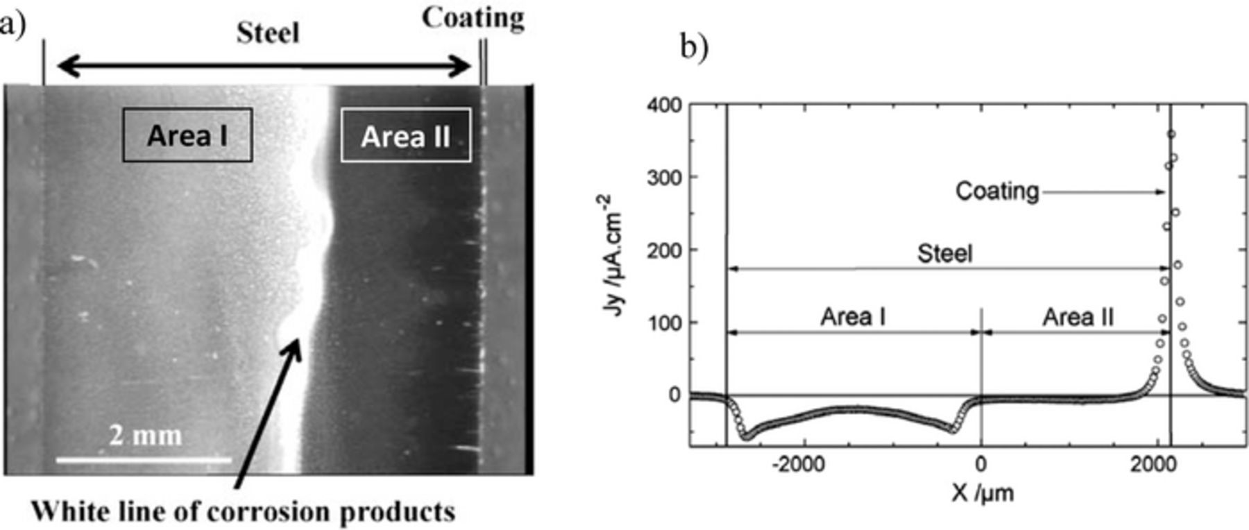
**Figure 7.** a) In situ optical image of the surface of HDG after 5 hours of immersion in 0.03 M NaCl. b) Experimental distribution profile of normal current densities at 50 μm above the sample after 40 minutes of immersion (Reproduced from Reference 93 with permission from Elsevier).

Painted metals

The application of SVET to characterize the corrosion on painted metals has received great attention but its use is limited to systems with defects. If the coating is in perfect condition, corrosion is absent and no currents are there to be measured. At later stages, underpaint corrosion may be taking place, and yet SVET might not be able to detect meaningful signals. For that, the current lines must reach the height of the probe. Fig. 8 shows two examples of painted metals analyzed by SVET. The map in Fig. 8a was measured above a blister of a degraded painted metal. The measurement was made far from the metal surface (current source) and the probe did not detect any significant signals. Another example is a transparent polymeric film applied on galvanized steel with a scribe exposing the substrate – Fig. 8b. SVET measured positive currents directly above the scribe. No negative currents were detected. This can be explained by a large cathodic region (leading to small cathodic current density of difficult detection) located mainly outside the mapped area. What is more important is that the transparent film reveals the corrosion of the metal substrate (otherwise hidden) with a pattern significantly different from that of the SVET map. Most of the currents developed beneath the polymeric film away from the scribe did not pass to the bulk of the solution. This shows that even when maps with coherent currents are obtained, SVET might not provide a complete description of the process occurring at the painted surface.

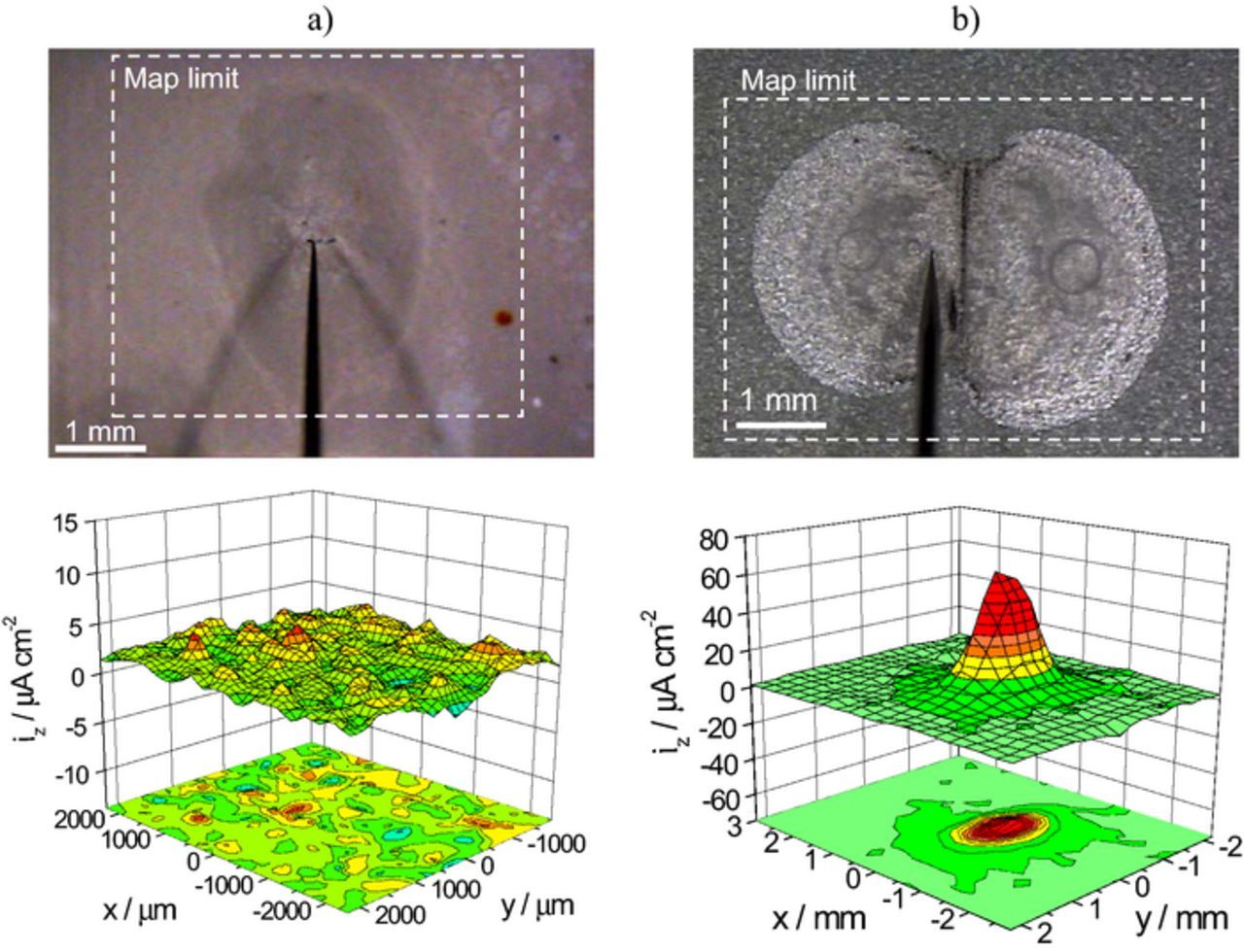
**Figure 8.** a) SVET map above a large blister on a painted metal (5 μm polyester primer + 15 μm polyurethane coating applied on electrogalvanized steel and immersed in 0.5 M NaCl during one month) measured in 0.1 M NaCl, b) SVET map measured in 0.1 M NaCl 200 μm above electrogalvanized steel coated with 5 μm transparent (unpigmented) polyester primer with a scribe down to the metal.

Instrumentation

Presently three companies supply SVET instruments: AE,⁸² Uniscan Instruments Ltd (marketed by Bio-Logic⁹⁹) and Princeton Applied Research (marketed by AMETEK¹⁰⁰). Hokuto-Denko (Japan) also produced a model in the 1990s. Other apparatuses have been developed by some research groups^{2,4,101–104} but only that developed at Swansea University remains with success.^{46,81,105–107}

All results presented in this paper were obtained with the SVET system from AE. The information that follows is based on this equipment. While the principle is the same for all instruments, the technical details are certainly different. The main particularities of the AE model compared to the others are the double vibration (X and Z), the probe tip size (10–20 micrometers for AE and more than 100 μm for the other systems) and the video camera positioned directly above the sample allowing the simultaneous acquisition of maps and surface images. This system was developed for applications in biology and is based on the instrument described previously (4). A schematics of the SVET system is presented in Fig. 9a). It consists of a video camera that allows one to control the probe position and obtain images of the sample, a three motor system to move the probe with 1 μm precision, a pre-amplifier and two lock-in amplifiers, one for each vibration. A second camera located laterally is optional. It is also possible to modify the system to move the sample instead of the probe. The vibrating electrode is connected to the end of a plastic arm which is fixed to a linkage with two piezoelectric vibrators responsible for the X and Z vibrations (with frequencies ranging from 40 Hz to 1000 Hz). The measurement is controlled by the ASET software developed by Science Wares, Inc. (USA).¹⁰⁸ An anti-vibration table, a Faraday Cage and an uninterruptible power source are recommended for optimal performance.

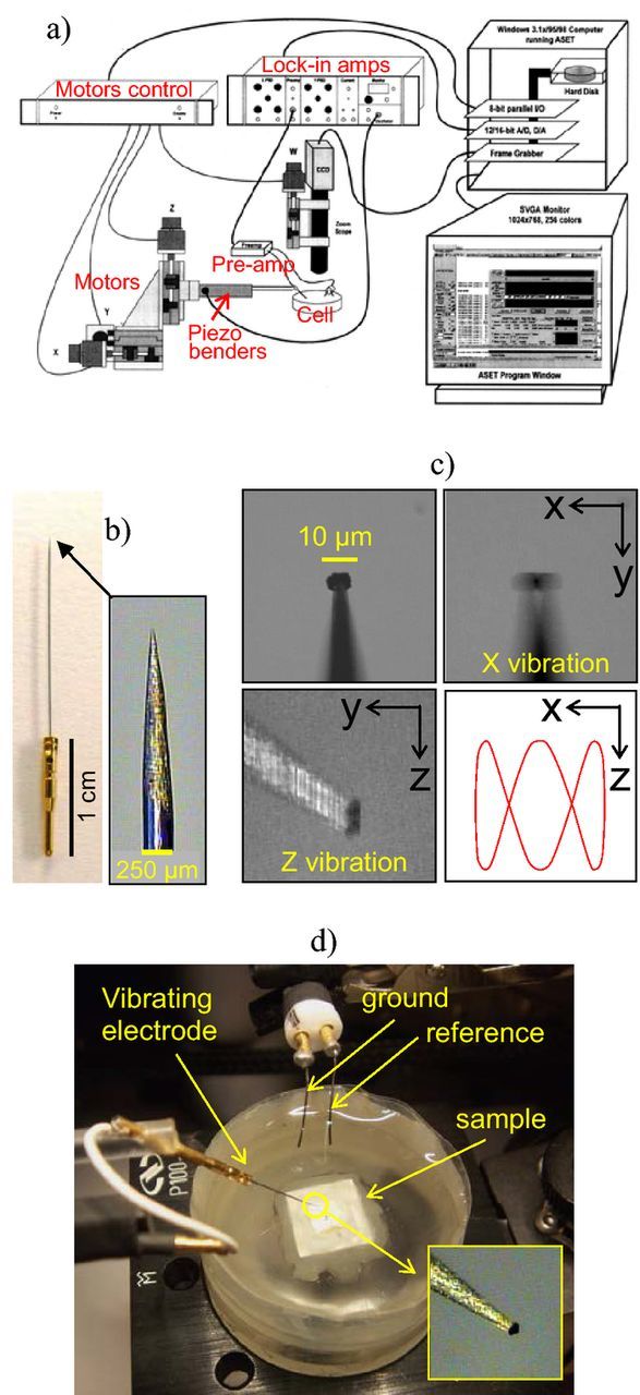
**Figure 9.** a) Scheme of the interaction between the different modules of the SVET system (taken from the ASET Manual 108), b) SVET microelectrode, c) vibrating electrode depicting the two vibrations and a sketch of a Lissajous figure with same amplitude in X and Z and frequencies of 1 Hz in X and 3 Hz in Z, d) electrochemical cell for SVET experiments.

Fig. 9b shows the tip of the vibrating electrode, usually a 80%/20% platinum-iridium needle 1.5 cm long and 225 μm in diameter, thinned at its end and coated by 3 μm layer of Parylene-C polymer applied by CVD. The electrode tip is a hemisphere of 1.5–2.5 μm radius and is the only point where the insulating film was removed by a voltaic arc. These electrodes are produced by Microprobes Inc. (USA)¹⁰⁹ and the main application is neural recording and stimulation. To be used as SVET probes, the electroactive area of the tip is increased by electrodepositing a small platinum black sphere of about 10–20 μm in diameter – Fig. 9c. The typical electrochemical cell is shown in Fig. 9d. The sample is placed in an epoxy holder of 3 cm in diameter and insulated except for the area to be mapped. Tape wrapped around the epoxy mount provides the solution reservoir – Fig. 10a. The potential is measured between the vibrating electrode and a platinized platinum wire that works as reference. A second wire is the ground of the dual n-channel field effect transistor (JFET U401) that lies inside the pre-amplifier and is the core of the SVET measurement.

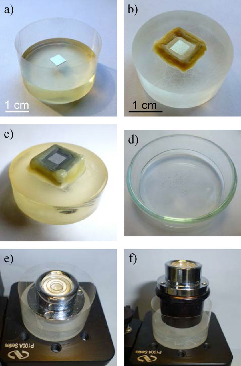
**Figure 10.** Sample mounts: a) for bulk materials, b) and c) for coated specimens, d) Petri dish for powder or particulate materials, e) bubble level to align flat samples and f) to align coated samples.

Samples

Fig. 10 shows examples of the most typical samples and cell preparation for the AE equipment. Other systems usually have larger solution pools. Homogeneous bulk materials can be embedded in inert matrices like the epoxy mounts presented in Fig. 10a. The greatest advantage is that after a sequence of tests, the surface can be polished and is ready for subsequent experiments. Crevices between the sample and the mount must be checked and avoided. Coated samples cannot, in general, be embedded and are glued to the polymeric mount, as shown in Figs. 10b and 10c. The cut edges must be insulated to avoid galvanic coupling between the coating at the top and the base material at the edges. In fact, all samples should be isolated except for the area to be mapped. Varnish, insulating tape or beeswax are used for this purpose. Powder or particulate materials can be measured in a Petri dish – Fig. 10d.⁶⁵ The solution reservoir is usually made with adhesive tape around the epoxy holder. So far there are no reports of any changes in the testing solution introduced by the tape. The volume of solution is usually in the order of 5–7 mL and the height of solution above the sample surface is around 7–10 mm. This is small and might be a problem with very reactive samples or for long time experiments. In the first case, changes in pH and in concentration of metal cations from the metal oxidation can modify the testing environment, alter the kinetics of the process and lead to erroneous conclusions. In the latter case, water evaporation can concentrate the electrolyte or inhibitors, also affecting the results. Different approaches exist to solve the problem. The most simple is to test the sample for only a few hours. However, longer periods are often necessary to extract meaningful information. The electrolyte solution can then be renewed with fresh portions but the forced convection may also affect the kinetics of the process. Alternatively, the volume can be increased by connecting the solution reservoir to a second vessel thus maintaining a large pool of solution. Another practical way of controlling the evaporation during measurements while the sample is being tested is to monitor the focus of the surface image. Water evaporation brings the image out of focus. Addition of water drop by drop until the focus is regained brings the solution to the initial level. In studies prolonged for weeks or months, the samples can be stored in a humidity chamber to prevent evaporation.

Measurement Sequence

The following description is valid for the AE equipment. The sample surface must be aligned parallel to the plane of the SVET measurement. This is accomplished by using a bubble level – Figs. 10e and 10f – with the help of the video camera. Then it is necessary to tell the system the position of the tip. The probe is brought to the surface until it touches it. This will be the zero level in Z axis. The approach of the tip to the surface is done with the help of the video camera and movement on the micrometer level. When the probe touches the surface, any new movement downwards forces the probe to slide to the front which is detected in the video image. The approach should be done not on the metal surface to avoid galvanic coupling with the Pt deposit. Besides, small pieces of broken Pt black threads can stay on the surface forming permanent local cathodes.

With the tip on the surface, the operator points the position of the tip in a software window that displays the video image of the surface. The video camera has several magnifications and the system is calibrated for each one, so that by pointing the position of the tip the system immediately identifies its position in X and Y. Z is assumed to be zero by default, which is why the probe tip has to be at the surface during this step.

The measurement starts always with a reference point, acquired in the bulk of the solution where no current flows. The reference values in-phase and quadrature for each vibration should be very small, close to zero. They are subtracted from all subsequent experimental points. Higher reference values are indicative of an electrode in bad condition and is pointless to continue until the problem is solved. Usually this is fixed by re-plating the platinum black deposit.

The most typical SVET measurement is a collection of points in the form of a map parallel to the surface. Maps normal to the surface can also be acquired. Lines provide faster measurements and can be parallel to the surface crossing the areas of interest or can be approach lines from the bulk to the surface. In very particular cases, it may be preferable to follow a pre-programmed path to contour the shape of the sample or only analyze selected points of the surface without the need of a complete map. Another possibility is to place the tip in a fixed position above one point of interest (a defect, a pit, or another feature at the surface) to measure the evolution of the process over time or after a modification has been produced in the system (change in solution pH, O₂ or Cl⁻ concentration, addition of inhibitors, or other).

A last point that cannot be overstated is the need for the electrode tip to have a good platinum black deposit in order to yield low noise measurements. This is crucial for good quality data. The absence of this deposit usually leads to useless data. A routine exists to diagnose the tip quality^101,110 and it should be run at the beginning of any set of experiments or when maps show no currents or high noise. In this test, a signal is injected through the probe and monitored in an oscilloscope permitting to estimate the tip capacitance. The higher the better but 1 nF is already acceptable for the common tips used (Fig. 9c) and for the AE equipment. In fact, the minimum SVET tip capacitance (and hence maximum interfacial impedance) permissible for useable SVET measurements depends upon the input characteristics of the SVET signal amplifier and the amount of noise entering the experimental cell from the electrical environment, so it is instrument dependent.

Experimental Parameters

The following parameters are the most important for the SVET operation:

(1)
The amplitude of vibration is usually set when the instrument arrives. Afterwards, even with tips of different sizes, the amplitude remains unchanged. Naturally, if the amplitude is changed re-calibration is mandatory. Typical amplitudes range between 5 μm (Fig. 9c) and 30 μm.⁸¹ Higher values give better sensitivity but also have problems associated – see Effect of vibration section, particularly 6).
(2)
The frequencies of the X and Z vibrations are chosen in the first use of the equipment and, in general, there is no need to change them. It is important to choose frequencies that do not induce vibration in the orthogonal directions, avoid resonance frequencies, the frequency of the powerline and its harmonics. Apart from that, any frequency can be used.
(3)
The sampling rules include the so called wait and average times. When the probe reaches a position of measurement it waits some time (wait time) for the sample recover from the disturbance induced by the probe motion and then acquires signal for a given time (average time). Typical values of both wait and average times vary between 0.02 s and 1 s.
(4)
The tip size ranges from 10 to 30 μm in diameter of the Pt black deposit. Other sizes are possible but rare. In principle there is no obstacle in reducing this size as long as the probe does not get noisy, which is the main reason for using larger tips. Some systems use bigger probes as, for example, a 125 μm diameter platinum disk without platinum black deposit, sealed in glass sheath giving a final 250 μm diameter tip.⁸¹
(5)
The distance to surface is important because it determines to a great extent the spatial resolution. Typical values are from 100 to 200 μm, but any other distance is admissible. For higher distances, the sensitivity to the current decreases rapidly (Fig. 3). Lower distances increase the risk of the probe touching the surface or corrosion products. Also, an overestimation of the true field as the probe gets very close to the surface was reported by Isaacs¹¹¹ (Effect of vibration section). According to that study, to avoid current overestimation, the probe should be away from the source at least four times the amplitude of vibration. Another issue is the shielding effect produced by the probe when it is close to the surface. As illustrated in Fig. 9, when tips with 10–30 μm diameter are scanning at heights of 100–200 μm, this effect is negligible.
(6)
The number of points is important for the map definition. The larger the better but this is time consuming and a compromise must be attained. Typical maps range from 10 × 10 to 100 × 100 points and the most common are from 20 × 20 to 50 × 50. Fig. 11 shows the effect of the density of points and distance to the surface on the spatial resolution and map definition. The sample is a zinc-iron galvanic couple. While the cathodic activity at the iron is fairly uniform, the corrosion on zinc is localized and does not cover the total area of the electrode. In the SVET maps of Fig. 11, the closer the tip is to the surface the better is the spatial resolution. For maps with distance between points the same as the distance to surface, a higher number of points improves the map definition (better delineation of the map details) but has no advantage regarding the spatial resolution. This is further discussed in the Spatial resolution section.

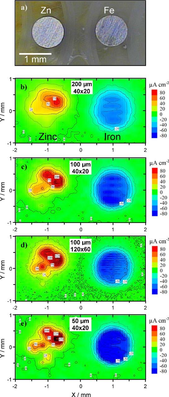
**Figure 11.** Effect of distance to surface and number of points in map resolution. Reproduced from Reference 120 with permission from Elsevier.

Operational Details

Sensitivity

SVET sensitivity is the smallest current that can be discriminated above the noise level.

The noise level can be determined from maps acquired in the same experimental conditions as regular measurements but without currents flowing in solution. One example is the map shown in Fig. 12a which was measured in a Petri dish. The current density is randomly distributed between −1 and +1 μA cm⁻². Fig. 12b presents the values of the experimental points in the map with lines indicating the mean value ( = 0.082 μA cm⁻²) and the standard deviation (σ = 0.49 μA cm⁻²). Also plotted are lines for two and three times the standard deviation. The value of ±1 μA cm⁻² (the mean value plus two times the standard deviation) was considered a good indication of the noise level for the experimental conditions of this example.¹¹²

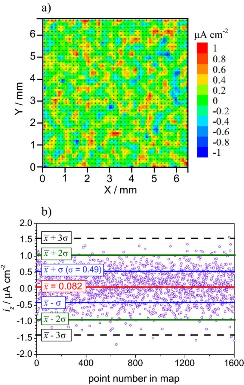
**Figure 12.** a) SVET map (experimental points in black) measured in a Petri dish containing 0.05 M NaCl (no currents flowing in solution) and b) values of the experimental points in the map with the mean value () and standard deviations (σ, 2σ and 3σ).

**Figure 12.** a) SVET map (experimental points in black) measured in a Petri dish containing 0.05 M NaCl (no currents flowing in solution) and b) values of the experimental points in the map with the mean value () and standard deviations (σ, 2σ and 3σ).

Only values higher than the noise level are considered significant, i.e., associated with the flow of current. Table I presents the noise level of SVET measurements in three common solutions. It is clear that SVET sensitivity depends directly on the medium conductivity. In pure ethanol it was possible to measure current densities of nA cm⁻² over iron and zinc.¹¹³ Equation 3 can be used to correlate the minimum current discriminated by SVET with the conductivity of the medium. In all cases, for a peak to peak amplitude Δr = 10 μm, the same potential difference between 160 and 180 nV is encountered (ΔV in Table I), which can be considered as the detection limit of the equipment used in these experiments.

Table I. Sensitivity in diverse solutions and distances to a point current source.

				Minimum current (nA) at the
		Noise level		source necessary to be detected at
C_NaCl (mol dm⁻³)	κ (S cm⁻¹) (23 ± 1°C)	( ± 2σ) (μA cm⁻²)	ΔV (nV)	100 μm	200 μm
0.5	4.54 × 10⁻²	7.5	165	19	75
0.05	5.55 × 10⁻³	1	180	2.5	10
0.005	6.02 × 10⁻⁴	0.1	166	0.25	1

In the SVET context, sensitivity may also mean the minimum current at the source that can be detected. In this case, the source-probe distance is also an important factor. Table I gives experimental values of the minimum current flowing from a point current source (similar to Fig. 3a) that can be detected by SVET at the typical testing distances of 100 μm and 200 μm. According to Table I, in 0.05 M NaCl, the limit of detection is 1 μA cm⁻² and SVET is able to detect a current of 2.5 nA at the source when it is at a distance of 100 μm. If the probe is 200 μm away from the point source, it can only detect currents higher than 10 nA at the source. Note also that this example is for a point source with the current being distributed in all of the volume. If the point source is at an insulating surface, then the volume is halved and so is the minimum current at the source susceptible of being detected.

Spatial resolution

This can be defined as the smallest distance between two point sources that can be resolved by SVET. A simple rule is to consider that SVET will discriminate two sources when it is at a height half of the distance between them. This means that a probe 100 μm above the surface will only differentiate point sources that are at least 200 μm apart. Or, to distinguish two points separated by 10 μm, the probe must be at the most 5 μm above the surface, which is impossible for common SVET probes of 10 μm size and 5 μm vibration amplitude (20 μm peak-to-peak).

Isaacs showed that the signal measured by SVET is the same above a point source or a disk, when both are driving the same current (not current density), and the probe is at distances higher than the disk diameter.¹¹⁴ As an example, if the measurement is made with the probe 100 μm above the surface, the SVET map will show the same round shape whether the source is a point source or a disk of 100 μm diameter (or in fact any shape smaller than the disk perimeter) provided the current from the source is the same. To identify the correct shape the probe must approach the surface.

Isaacs also showed that for an SVET scanning at a constant height (h) directly over a point current source, the "width at half maximum" (whm) of the SVET signal-distance response curve is whm = 1.533 h.¹¹⁴ This compares with the whm = 3.46 h for SRET^19,73 and is one of the principal reasons for the improved performance of SVET relative to SRET. It also means that there is no practical advantage in reducing the diameter of the SVET tip (electrochemically active portion) to much less than the experimental scan height.

Effect of vibration

The vibration of the probe is associated with several important effects that must be acknowledged:

(1)
The first refers to the capability to stir the solution and homogenize the local chemical composition. This effect was studied by Lucas and Ferrier who concluded that the convective vortices created by the electrode vibration change the concentration of chemical species close to the electrode tip but not the local current density.¹¹⁵ The homogenizing action occurs around the tip and rarely affects the composition of the solution in contact with the surface. The same conclusion was reached in a recent study for the SVET system used in this work.¹¹⁶ This effect, however, is strongly dependent on the probe size, probe-surface distance and amplitude of vibration.
(2)
The local homogenization by the probe vibration has an important effect in cancelling concentration gradients that could otherwise lead to differences in Nernst equilibria at the two ends of the vibration, eventually affecting the potential sensed by the SVET. Since the probe tip is a Pt-black electrode, it can sense any redox equilibria at its surface like any other platinum electrode.¹¹⁷ It has been suggested that this effect remains during SVET operation (when it vibrates) and could be responsible for the mismatch in positive and negative currents in SVET maps.¹¹⁸ However, as discussed by Dolgikh et al.,¹¹⁶ the vibration cancels the concentration gradients around the vibrating electrode and the differences in Nernst equilibrium at the two ends of vibration should be negligible. This in fact was already acknowledged by Jaffe and Nuccitelli² and by Ferrier and Lucas.¹¹⁵
(3)
Close to the current source the ionic concentration is highest and decreases with the diffusion of ions until a constant value is attained in the bulk of the solution. The solution conductivity is a reflection of the ionic concentration. Therefore it is constant in the bulk but increases close to the surface, inside the diffusion layer. The calibration assumes the bulk conductivity and currents measured inside the diffusion layer can be underestimated because the correct conductivity is not used. However, the local mixing provoked by the probe vibration minimizes the difference in local and bulk conductivities. Moreover, even without local mixing, simulations indicate that the local conductivity is only 10% higher than the bulk conductivity at a distance of 50 μm from a point source and 50% higher at 10 μm from the source.¹¹⁹
(4)
The local mixing induced by the probe vibration has a fundamental and extremely important effect in the SVET output. The suppression of concentration gradients around the probe minimizes the diffusion current and, as a result, the migration current becomes close to the total current, even inside the diffusion layer.¹¹⁶ This explains why SVET measures the total current density irrespectively of the distance to the electrode, while standard calculations predict a strong decrease of migration current inside the diffusion layer with a concomitant increase in diffusion current. Fig. 13 compares the standard calculations with simulations that consider the local mixing effect by the probe. Fig. 13a presents the results of standard calculations together with the experimental current density measured by SVET in an approach line from the bulk of solution to the surface at the center of a 270 μm diameter platinum disk driving an anodic current of 60 nA. The SVET results are very close to the total current which is dominated by the diffusion component at distances smaller than 400 μm. For bigger distances, the diffusion decays to zero and the migration coincides with the total current. According to the standard calculations, SVET (which measures the migration current) should give very small currents as it approaches the current source. However, in practice, the values are close to the total current. Recent calculations took into account the local mixing induced by the vibration and radically different results were obtained.¹¹⁶ Fig. 13b shows the total current density and the migration current from standard calculations together with the migration component calculated considering the local mixing when the probe is placed at 250 μm, 100 μm or 30 μm from the surface. In any of these positions, the probe vibration mixes the solution in its very vicinity, levelling the local solution composition and leading to the local decrease of the diffusion component and increase of the migration component. This is why the SVET still measures a value close to the total current even inside the diffusion layer. The results are still qualitative but give a clear indication of the impact of the mixing in the current density that is actually measured by the SVET.
(5)
It was stated above that the probe vibration mixes the solution close to the tip but its effect rarely reaches the surface of the sample. This, however, is strongly dependent on the probe size, probe-surface distance and amplitude of vibration. In fact, conditions have been reported in which the amplitude of vibration was so large that it enhanced the convective transport of dissolved oxygen toward the surface resulting in a fourfold increase in the cathodic current.¹⁰⁶ An investigation with the SVET probe used in this work showed that the vibration has no important effect under normal measurement conditions, but revealed significant convection induced by the probe movement during scanning.¹²⁰
(6)
Isaacs studied the relation between vibration amplitude and distance to the source and concluded that when the probe is at distances to the source closer than four times the vibration amplitude, the measured signal overestimates the true signal.¹¹¹ For the typical SVET equipment used in this work, this problem only appears when the probe is closer than 40 μm from the surface.
(7)
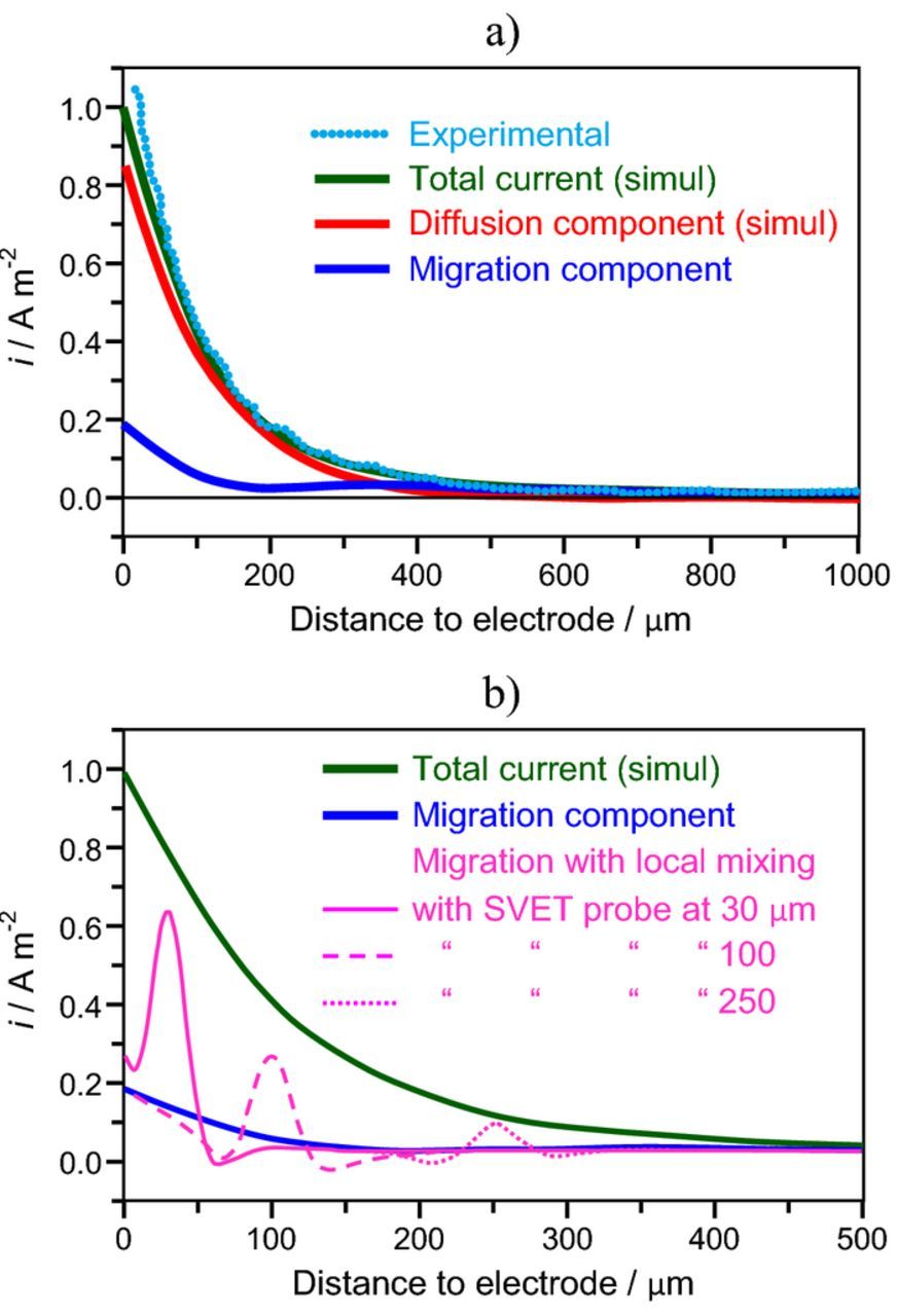
A last aspect is the risk of misalignment between the axis of vibration and the normal to the surface. Studies in the literature indicate that deviations up to 20–30° are not significant.^19,121

**Figure 13.** a) Experimental SVET measurements and simulations of the total current density, diffusion and migration components along a vertical line at the center of a disk source of 270 μm diameter and I = 60 nA; b) total current density and migration current both calculated by standard simulations and migration current calculated considering the local mixing induced by the SVET probe when it is at 30, 100 or 250 μm above the surface of the electrode. Adapted from Reference 116 with permission from Elsevier.

Towards Quantification

SVET is a good technique to image the evolution of corrosion at a metal surface. Often it is desirable to go further and try to use the SVET results to obtain quantitative data and even to determine corrosion rates. This section addresses some of the calculations that might be possible with SVET data. Consider Fig. 14, depicting an optical image and a SVET map of the localized corrosion of 2024-T3 aluminum alloy after 1 day of immersion in 0.05 M NaCl. Anodic (red) and cathodic (blue) regions are distributed along the surface. The map of current densities is very much coincident with the attacked regions displayed in the optical image which means the activity stayed in the same location since the beginning of immersion.

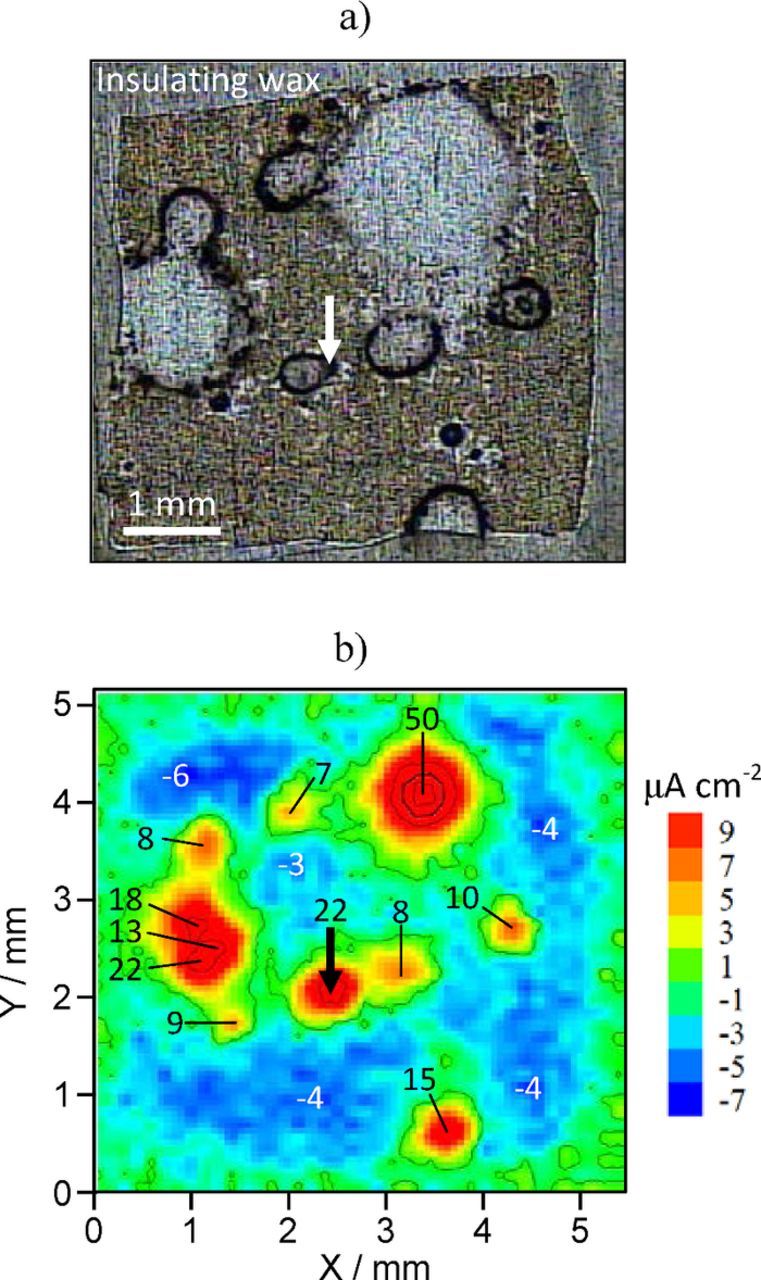
**Figure 14.** a) Optical image of the surface of AA2024-T3 after 24 hours of immersion in 0.05 M NaCl and b) SVET map acquired 200 μm above the surface at the same time of immersion. (Experimental details in Supplementary Material).

Current in a single point measured by the SVET

The current density at the point indicated by an arrow in Fig. 14 is 22.23 μA cm⁻². This means that the electrical field sensed by the SVET probe in that point is the same as the electrical field generated by a 22.23 μA current passing in 1 cm² in a medium with the same conductivity. To know the absolute current passing in this particular point, it is necessary to know the area corresponding to the point, which can be obtained by dividing the map area by the number of points. In this example the map area is 0.5464 cm x 0.5126 cm = 0.2801 cm² and the number of points is 40 × 40 = 1600. The area corresponding to each point is 1.75 × 10⁻⁴ cm². The absolute current in this point is then (22.23 μA cm⁻²) × (1.75 × 10⁻⁴ cm²) = 0.00389 μA (3.89 nA). More points mean better map definition, but the total current and the current density, obviously, remain the same.

Correlation between the current measured in solution and the current at the source

SVET measures the ionic currents that cross a plane above the corroding metallic surface, typically at a height of 100–200 μm but, in general, it is the current that crosses the metal-solution interface that is of interest. It is not easy to correlate these two quantities. In fact, it is simple only in the case of a point current source. If the point source is embedded in a non-conductive flat surface, the current I flowing from this point that gives origin to the current density measured by SVET, i_SVET, is given by,

where r is the source-probe distance and 2 π r² is the area of the hemisphere of radius r. The SVET maps usually show only the Z component of the current density. Exactly above the point source the Z component coincides with the current density vector because the X and Y components are zero at this position. If the point marked in Fig. 14 is a pit surrounded by a cathodic area, it may be treated as a point current source, Equation 6 can be used, and I = (22.23 μA cm⁻²) (2) (π) (200 μm)² = 55.87 nA. This is the value for a point on the surface. The total current at the sample depends on the activity of all points.

Determination of the overall sample current

Two approaches are described to estimate the total current of the sample in order to determine the corrosion current density comparable to what is obtained with other electrochemical techniques. Basically, the corrosion rate expressed in terms of current density is the anodic current of the sample (at open circuit potential) divided by the area of the sample that is exposed to the testing medium. The first approach might be used when maps contain just a few, intense, well defined and well separated round shaped points. If the corrosion of the sample is due only to the activity on those points, the summation of all individual point currents (calculated by Eq. 6) leads to the total corrosion current of the sample. Dividing it by the exposed area gives the corrosion current density. The map in Fig. 14 depicts 11 pits (3 are almost merged in a spot at the left of the map) and the summation of their currents calculated from Equation 6 is 0.4743 μA. The exposed area of the sample is 0.19 cm². The corrosion current density is then 2.5 μA cm⁻².

A different approach must be used when, instead of well separated round shaped points, the map is composed of wide and irregular regions of variable current density, which is the most common case. The approach works only when the current flows from the surface in a planar fashion (no radial components) and the map is coincident with the exposed sample area. When these conditions are met, the current density distribution in the map should closely reflect the current at the metal surface. The corrosion rate corresponds to the average positive current density in the map, determined by,

where i_n(an) is the current density of each positive (anodic) point in the map and P is the total number of points in the map. Alternatively, it is possible to sum the currents (not current densities) of all positive points, giving the total positive (anodic) current in the map, and divide it by the sample area, as in the following equation,

where A_point is the area corresponding to one point and A_sample is the exposed area of the sample. The product of each local current density and the area of one point is the current passing in the area corresponding to that point. Summing the currents of all positive points gives the total positive current in the sample. Dividing it by the area of the sample returns the anodic current density (corrosion rate). If the area of the map is used instead of the exposed sample area, Equation 8 becomes Equation 7. These equations use the discrete values measured in each point, yet the same can be obtained by numerical integration of the positive area of the generated map.⁸¹ Moreover, the equations are written for the anodic (positive) points but, in principle, the calculation can be done with the negative points as well.

When applying these equations, it is important to use only the values above the noise level to avoid current overestimation, especially in maps containing large number of points. If the above equations are used without attending this, they will return a positive value even in the absence of current. The noise level in Fig. 14 is the same as in Fig. 12 because the experimental conditions were the same. Therefore only values of magnitude higher than |1| μA cm⁻² should be used in Equations 7 and 8.

Table II shows the corrosion current density calculated by the different approaches presented above: sum of the individual anodic spots determined by Equation 6, map average of the positive or negative currents (Equation 7) and total current in sample divided by the sample area (Equation 8), taking into account only the points with current density higher than |1| μA cm⁻². The values in the table are close but are not the same. One important observation is the mismatch between positive and negative currents. They should be the same and cancel out but this is seldom observed in SVET maps. Reasons are given in the next section.

Table II. Corrosion current density determined by analysis of SVET map of Figure 14.

		Map average (Eq. 7)			(Eq. 8)
	Sum of currents of individual anodic spots (Eq. 6)	+ points	−points		+ points	−points
Corrosion current density (μA cm⁻²)	2.5	1.3	1.8		1.9	2.7

The corrosion rates in Table II are to be compared with values obtained by the global averaging electrochemical techniques (polarization resistance method, Tafel extrapolation, electrochemical impedance spectroscopy). Corrosion rates like these, associated with the total test area of the sample, work for cases of uniform corrosion but are not acceptable for localized corrosion as is the case of Fig. 14. Such values are misleading and can be dangerous because they give the impression of a rate of metal dissolution uniform in all surface when in fact most of it is concentrated in just a few points. What matters from the materials design and safety points of view is the depth of pits, particularly the deepest one. This information cannot be given by global techniques. In SVET maps, the peak with the highest current density corresponds, in general, to the deepest pit. This current can be used to estimate the local mass loss and penetration depth, but factors like the constancy of the pit current over time and the pit shape beneath the surface, are required for a correct estimation.

Limitations

The previous calculations do not give accurate results, but are underestimations of the true current, due to six main reasons:

(1)
The measurements are not performed with the probe at the surface but at a certain distance above it, typically 100–200 μm. SVET misses the currents that flow between anodes and cathodes below the measurement height, as shown in Fig. 15a.
(2)
The current that ascends and crosses the measurement plane will return to the surface through the same plane. The return path may be outside the mapped area and that current will not be measured, as shown in Fig. 15b.
(3)
The third reason is related to the technique sensitivity. The noise level in the typical solutions used for testing (0.01–0.1 M) is around 1 μA cm⁻². Lower currents pass unnoticed. An example is the case of a sample with anodic activity so localized that it is easily detected, while the cathodic activity is spread through the rest of the surface and the current density becomes smaller than the limit of detection.
(4)
The current flows in the three directions in space (the current density is a 3D vector) but SVET measures either one or two of them and usually only the Z component is used. As a consequence, the presented current density is an underestimation of the true current.
(5)
The movement of the SVET probe and, sometimes, the vibration itself, can enhance the transport of oxygen to the surface.^106,120 At the anodes, the effect is small but when the probe is scanning above the cathodes it enhances the transport of the cathodic reactant (O₂) precisely when it is measuring the cathodic activity. This might lead to an overestimation of this activity and to an unbalance between anodic and cathodic currents in the same map.
(6)
The calibration conditions must be satisfied at all times during measurement, that is, the measured potential difference is converted to the true local current density only when the conditions of measurement are the same as those used in the calibration.

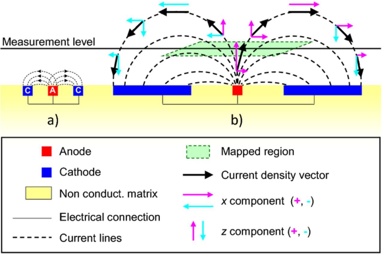
**Figure 15.** Scheme with some limitations of the SVET measurements.

Most of the above considerations explain the mismatch of positive and negative currents that are frequently observed in SVET maps. This section leads to the conclusion that SVET should be seen as a semi-quantitative technique to visualize corrosion, not really an alternative method to determine corrosion rates.

Modelling and Simulation

Part of the above limitations can be overcome by using numerical modelling and simulation. This is mandatory to model the actual current distributions at the surface of the electrodes and accurately relate them with the measurements in solution. Usually finite elements or boundary elements methods are used. Models vary from the more simple electrostatic or potential model, based on the Laplace equation and considering only potential gradients in a medium of uniform conductivity,^{93,95,122–128} to more rigorous treatments contemplating the electrochemical gradients resulting from transport and reaction of chemical species in the solution using the Nernst–Planck equation.^{94,96,116,119} With this model, not only current and potential are modelled but also the local chemistry, including the distribution of pH, O₂ and corrosion products. An illustrative example of the application of numerical modeling of SVET results can be given for the cut-edge corrosion presented in Fig. 7. This system has been numerically simulated by the two models. Using the electrostatic model,⁹³ thanks to the convection induced by the microelectrode vibrations which removed local concentration gradients, the steady state current distribution measured by the SVET was simulated taking into account a ternary current distribution on the steel surface. The only discrepancy was observed in an asymmetrical distribution of cathodic current that was measured but not simulated. The asymmetry was attributed to the diffusion potential component of the electric field that cannot be treated by this model. A second model, that was called coupled electrochemical-transport-reaction model (CETR model),⁹⁴ was able to resolve the discrepancy. Fig. 16a shows the closeness between experiment and simulation. The contribution of each ionic species to the diffusion potential is represented in Fig. 16b. Only the species of the supporting electrolyte, sodium and chloride ions, lead to a positive diffusion potential above the cathode, and are responsible for the increase of the cathodic current at the Area I/Area II interface (the discrepancy not resolved with the previous model). Interestingly, both models simulate accurately the SVET response only in the absence of a stagnant layer at the electrode surface, i.e. in strong convective conditions. This is because when SVET measurements are performed in the vicinity of the cut-edge surface, convection resulting from probe vibrations annihilates (only locally) diffusion layer effects. Then it can be considered that SVET measurements are performed in a homogeneous medium (absence of concentration gradients). In non-convective ("natural") conditions, the CETR model can be used to simulate not only the total current distribution (in absence of convection induced by the microelectrode vibrations), but also other variables such as pH gradients in the diffusion layer.^94,96

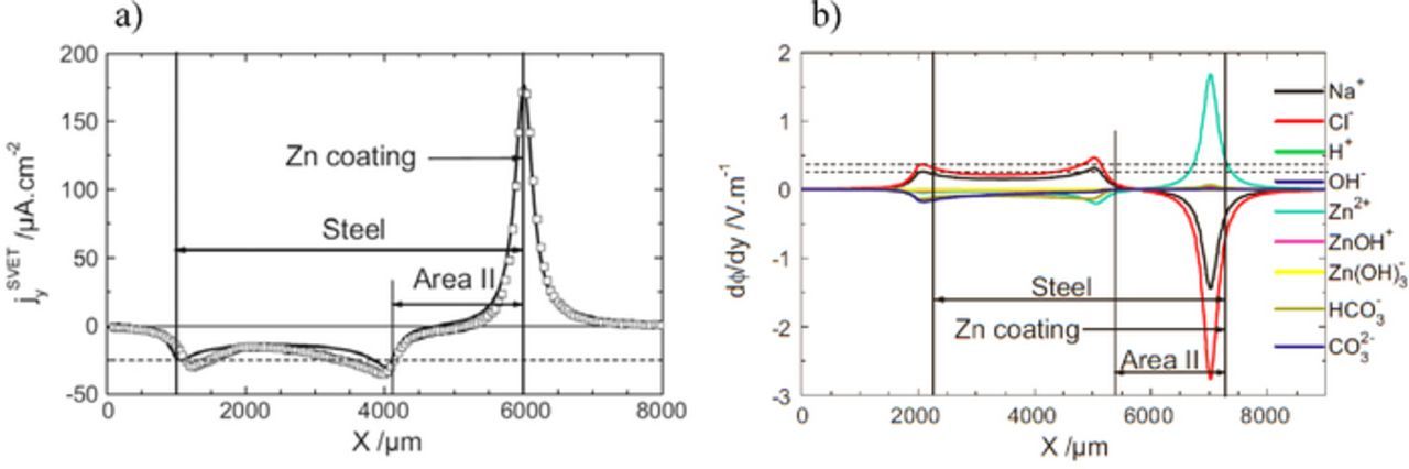
**Figure 16.** a) Normal current density profiles 150 μm above the cut-edge (see Fig. 7); squares: experimental profile; solid line: simulated profile with the CETR model assuming no diffusion layer and cathodic inhibition over a distance of 1900 from the zinc surface; b) Simulated contributions of ionic species on the normal component of the diffusion potential 150 μm above the cut-edge surface with cathodic inhibition on a part of the steel surface (Area II in Fig. 7) without the diffusion layer (Reproduced from Reference 96 with permission from Elsevier).

Apart from numerical modeling, it should be mentioned at this point a set of papers published in the 1950s by Wagner¹²⁹ and Waber^130–135 who analyzed mathematically the current and potential distribution in solution for various types of electrochemical cells, sometimes using data from previous works.^22–29 Other papers worth mention are those of Nanis and Kesselman,¹³⁶ Miller and Belavance,¹³⁷ McCaferty,¹³⁸ and Morris and Smyrl.¹³⁹ The SVET operation and response has also been modeled in several works.^{111,114,116,119,140–145}

Combination of SVET with Other Techniques

Complementarity with potentiometric and amperometric microelectrodes

SVET measures the ionic currents in solution but no information is given about the actual chemical species involved in the process. This important piece of data can be provided by potentiometric and amperometric microelectrodes. An example of the complementary use of SVET with the potentiometric measurement of pH and amperometric measurement of dissolved O₂ is now presented (Experimental details are given in the Supplementary Material). Fig. 17a shows a sample of 2024-T3 aluminum alloy coated with a 2 μm thick film produced by the sol-gel method. The surface of the sample was insulated with beeswax except for a window of 3 × 3 mm² and two small defects were produced in the sol-gel film so that the metallic substrate was exposed to the solution only on those two points. The sample was left corroding for 20 hours in aqueous 0.05 M NaCl and then crystals of cerium nitrate (corrosion inhibitor) were added to the solution in the exact amount to achieve a concentration of 0.01 M in Ce³⁺. Fig. 17b presents the ionic currents in solution, the local pH and the O₂ reduction current before and after the addition of inhibitor. The pH was measured with a potentiometric microelectrode and the reduction current of dissolved O₂ in solution was measured amperometrically with a 10 μm diameter platinum microdisk electrode polarized at −0.750 V vs Ag|AgCl|0.05 M NaCl electrode. The ionic currents before inhibition show a positive peak above one defect (anodic) and a negative peak above the other defect (cathodic). The solution pH increased above the cathodic defect (where OH⁻ is produced) but no change was detected above the anodic one. The O₂ reduction current was constant in solution except above the two defects, where it decreased. The decrease results from the lower local concentration of O₂ because it is being consumed at the metallic surface exposed by the defects. The fact that O₂ decreases in the two defects shows that the cathodic activity is taking place in both, including the one considered as anodic by SVET. The measurements performed 20 hours after the addition of inhibitor showed constant values in any point of the solution, either close to the surface or in the bulk of the solution. This is a result of the corrosion inhibition by formation of a surface layer of precipitated cerium oxides/hydroxides. The layer isolates the metal substrate from the environment, preventing any electrochemical activity and interrupting the consequent local chemical change of the solution. The full work is published elsewhere⁶³ and the results illustrate the benefit of combining different techniques to add partial pieces of information for a better characterization of the system under study. Many other examples can be found in the literature.^39,146–150

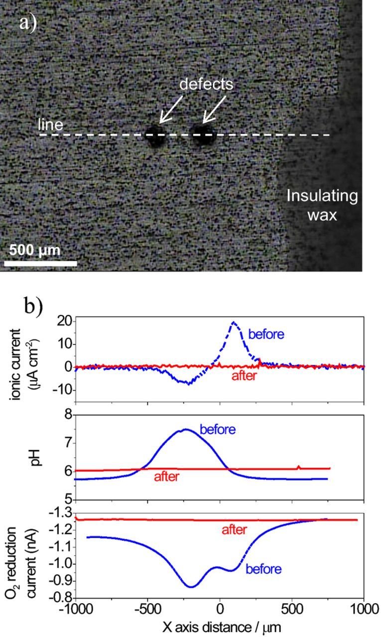
**Figure 17.** a) Aluminum alloy 2024-T3 coated by a hybrid organic-inorganic sol-gel film with two defects; b) SVET, pH and O₂ reduction current measured in a line above the defects 20 hours after immersion in 0.05 M NaCl and then 20 hours after the addition of a corrosion inhibitor (cerium nitrate). The SVET measurements were performed 100 μm above the surface and the pH and O₂ reduction current measured at 50 μm. (Experimental details in Supplementary Material). Adapted from Reference 63 with permission from Wiley.

Sample under external polarization

Potentiostatic or galvanostatic

In all cases presented so far, the samples were left corroding naturally, without external polarization. However, it is possible to polarize samples with a potentiostat while SVET measures the associated currents, as shown in Fig. 18 for the case of a pure Fe sample with SVET maps acquired at different fixed potentials. At the open circuit potential, anodic and cathodic regions are distributed over the surface. Anodic or cathodic polarizations promote, respectively, oxidation or reduction, with the current varying exponentially with the overpotential. Examples are given in the literature.^{38,113,150,151}

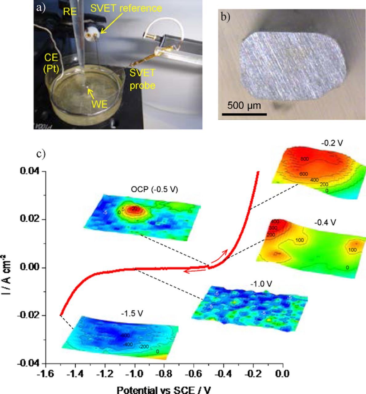
**Figure 18.** a) Electrochemical cell for SVET measurements under potentiostatic control (RE is silver-silver chloride reference electrode, CE is platinum counter electrode and WE is the sample to test), b) pure iron sample embedded in epoxy matrix, c) polarization curve of the pure iron sample in 0.1 M NaCl and SVET maps obtained with the sample polarized at different potentials. (Experimental details in Supplementary Material).

As an alternative to potentiostatic polarization, Williams, Birbilis and McMurray used galvanostatic conditions to study the hydrogen evolution on anodically polarized high purity magnesium, with the SVET.¹⁵²

Potentiodynamic

The final example is SVET measurements performed on a sample under potentiodynamic polarization. Fig. 19a shows the surface of a pure zinc specimen with the position of the SVET probe during measurements. Polarization curves were performed after a few hours of corrosion, necessary to the onset of clear and stable anodic and cathodic regions on zinc. Then, the potential was cycled between −1.25 and −0.9 V (vs saturated calomel electrode, SCE) at a scan rate of 10 mV s⁻¹, with the SVET probe placed in a fixed position in 2 points above the sample, A (anodic spot) and B (less active, mainly cathodic area), respectively. The curves are presented in Fig. 19b where "global" means the current measured by the potentiostat divided by the sample area and "local" means the current measured by SVET.

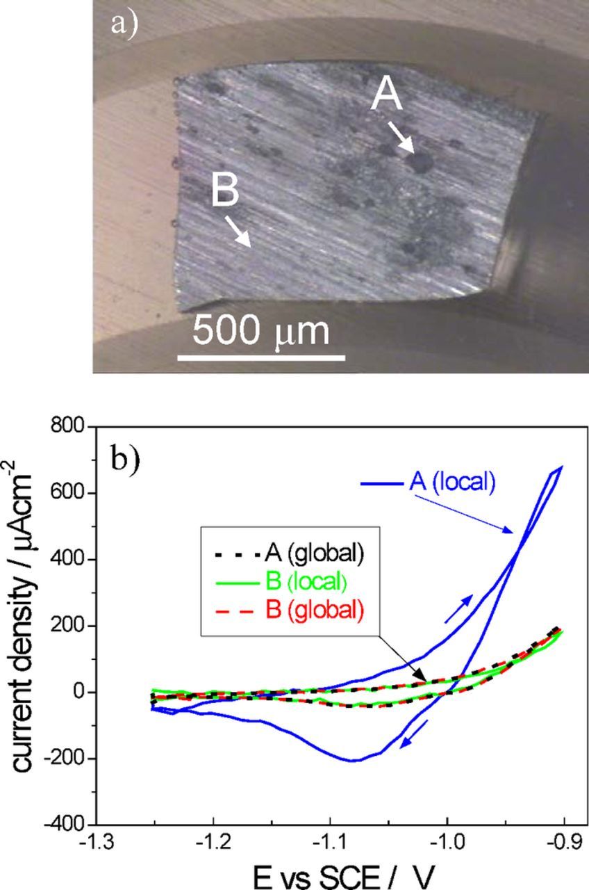
**Figure 19.** a) Pure zinc sample immersed in 0.1 M NaCl after testing, with the indication of the position of SVET probe during measurements: A (anodic spot) and B (less attacked area); b) Potentiodynamic curves obtained at a scan rate of 10 mV s⁻¹ with the global current measured with a potentiostat and the local currents in points A and B measured with the SVET. (Experimental details in Supplementary Material).

The global and local curves coincide except for the local currents obtained above the anodic spot where higher values were registered. This reflects the higher activity of this point of the sample. The negative peak corresponds to zinc deposition by the reduction of zinc ions formed in the anodic sweep. Some works can be found in the literature where SVET was combined with potentiodynamic polarization of the sample.^39,52,150

Concluding Remarks

This work is an introduction to the SVET and its application in corrosion research. All examples were selected for an easy perception of the basis of the technique, its particularities, advantages and limitations. The results and technical details are for one particular model of equipment because it is the one used by the authors, but the text is written to all interested readers and most of the information is valid for any SVET system.

SVET provides, in a single picture, the general overview of the processes occurring at the metal surface under corrosion. This information is unique and not given by any other technique. It should be seen as a technique to "visualize" corrosion and electrochemical events in general. Truly quantitative information requires caution and the help of modelling tools.

Expected future improvements are: i) simultaneous measurement of the electrical field in the three directions of space, ii) capability of scanning at a constant height from the surface, contouring the sample shape and roughness, and iii) use of smaller tips and smaller vibration amplitudes for higher spatial resolution. Also anticipated are improvements in simulation and modelling to better correlate the measurements with the processes at the surface and inside the diffusion layer.

It is hoped that these pages are enough for the understanding of the technique and to help the reader decide whether or not SVET can be beneficial for his work.

Acknowledgments

A.C.B. thanks University of Aveiro for the grant UID/CTM/50011/2013-CICECO. O.V.K. thanks Fundação para a Ciência e a Tecnologia (Portugal) for the PhD grant SFRH/BD/44475/2008. This work is dedicated to the memory of Hugh S. Isaacs (1936-2016).

Review—On the Application of the Scanning Vibrating Electrode Technique (SVET) to Corrosion Research

Article metrics

Author affiliations

Author notes

Dates

Abstract