
Abstract
Understanding the physical and chemical basis of device operation is important for their development. While hydrogen fuel cells are a widely studied topic, direct ammonia fuel cells (DAFCs) are a smaller field with fewer studies. Although the theoretical voltage of a DAFC is approximately equal to that of a hydrogen fuel cell, the slow kinetics of the ammonia oxidation reaction hamper cell performance. Therefore, development of anode catalysts is especially needed for practical viability of the DAFCs. To study DAFC operation, specifically interactions between reaction kinetics and different transport phenomena, we developed a one-dimensional model of a DAFC and performed a sensitivity analysis for several parameters related to the cell operating conditions (e.g., temperature, relative humidity) and properties (e.g., catalyst loading). As expected, temperature and relative humidity were very important for cell power. However, while faster reaction kinetics improved the cell performance, simply increasing the catalyst loading did not always produce a comparable enhancement. These and other observations about the relative importance of the operating parameters should help to prioritize and guide future development of and research on DAFCs. Further studies are needed to understand and optimize e.g. humidity management in different scenarios.
Export citation and abstract BibTeX RIS

This is an open access article distributed under the terms of the Creative Commons Attribution 4.0 License (CC BY, http://creativecommons.org/licenses/by/4.0/), which permits unrestricted reuse of the work in any medium, provided the original work is properly cited.
List of symbols
| Symbol | Name/description | Unit |
|---|---|---|
| aw | Water activity | — |
| A | Catalytic activity for AOR | A g−1 |
| cw | Water concentration in AEM/ionomer | mol m−3 |
| d | Diameter | m |

| Diffusional force acting on species k | m−1 |
| Dj | Fick's diffusion coefficient of j | m2 s−1 |
| Dik | Multicomponent Fick's diffusion coefficient of species i and k | m2 s−1 |
| EA | Activation energy | J mol−1 |

| Equilibrium potential of OAR/ORR | V |

| Theoretical potential of AOR/ORR | V |
| EW | Ionomer equivalent weight | g mol−1 |
| fε,ionomer | Ionomer volume fraction of the void (non-catalyst-and-substrate component) | — |
| fk | Molar fraction of species k of dry gas mixture | — |
| F | Faraday constant | C mol−1 |
| i | Current density, magnitude | A cm−2 |

| Current density vector | A cm−2 |
| iv | Volumetric current source | A cm−3 |
| i0 | Exchange current density | A cm−2 |
| ji | Flux of species i, magnitude | mol cm−2 s−1 |

| Flux of species i | mol cm−2 s−1 |
| kH | Henry's law coefficient | mol m−3 Pa−1 |
| kK | Carman-Kozeny geometry coefficient | — |
| K | Rate constant | mol m−3 s−1 |
| L | Layer thickness | m |
| mcatalyst | Catalyst mass loading | g cm−2 |
| Mj | Molar mass of species j | g mol−1 |
| Mn | Effective molar mass of gas mixture | g mol−1 |
| p | Pressure | bar |
| pA | Absolute pressure | bar |
| pj | Partial pressure of species j | bar |
| Q | Volumetric gas flow rate | ml min−1 cm−2 |
| Qm | Gas mass source | kg m−3 s−1 |
| R | Gas constant | J mol−1 K−1 |
| Rj | Source or species j, reaction rate | mol m−3 s−1 |
| Rmem | Membrane resistance | Ω m2 |
| RH | Relative humidity | — |
| T | Temperature | K |

| Gas velocity | m s−1 |

| Diffusional molar volume of species j | — |
| VM,W | Molar volume of water | m3 mol−1 |
| xj | Mole fraction of species j (in humid gas mixture) | — |
| zj | Charge number of j | — |

| ORR charge transfer coefficient | — |
| εj | Volume fraction of component j | — |
| η | Overpotential | V |

| Applied potential | V |

| Potential in electrolyte | V |

| *NH2 equilibrium potential | V |

| Gas permeability of material | m2 |

| Hydroxide conductivity of ionomer | S cm−1 |
| μv | Dynamic viscosity of gas | Pa s s |
| μj | Ion mobility of species j | m2 V−1 s−1 |
| μj,v | Viscosity coefficient of species j | Pas |

| Viscosity coefficient of species j at reference temperature | Pas |
| ν | Stoichiometric coefficient | — |


| AEM/ionomer ionic conductivity | S cm−1 |
| ρj | Density of j | kg m−3 |
| λ | Water uptake in AEM/ionomer | — |

| Mass fraction of species j | — |
Hydrogen produced from water electrolysis is one of the primary candidates for the storage and transport of renewable energy, but its storage and transport pose a significant challenge. 1 Among other options, several hydrogen-containing molecules are studied as hydrogen carriers that would allow the storage and transport of a liquid at moderately low pressure. This would be considerably easier than transporting pressurised hydrogen gas which, for instance, can embrittle metal used to carry it and tends to escape vessels faster than any other gas. Carbon-based molecules, i.e. CO2 reduction, are a widely studied approach to this problem, 2–4 but they have the inherent problem of releasing CO2 in their combustion. Therefore, they would be truly CO2 neutral only if the CO2 used in their synthesis was captured from the air, and the current lack of mature CO2 capture technologies may limit the large-scale viability of CO2 reduction. 5–7
In addition to electricity and fuels, stable food supply is a fundamental cornerstone of a society. Much of the modern agriculture is based on the use of fertilizers, and ammonia (NH3) synthesis via the Haber-Bosch process. 8 As a hydrogen-containing molecule, ammonia is also considered a viable hydrogen carrier and fuel. Ideally, its oxidation produces only water and nitrogen, thus avoiding CO2 emissions, but production of N2O could cause significant greenhouse gas emissions and therefore needs to be avoided. 9 Liquefied ammonia is considered for use especially for heavy transport and shipping and it is one of the most balanced options for this purpose with reasonably high efficiency and energy densities. 10
Instead of being a mere hydrogen carrier, ammonia could be used as a fuel in a direct ammonia fuel cell (DAFC). The theoretical voltage of a DAFC at room temperature is about 1.17 V, very close to the 1.23 V of a hydrogen fuel cell (HFC), in theory enabling it to directly replace the latter in any application. However, in contrast to the HFCs, the DAFCs carry the penalty of the slow kinetics of the ammonia oxidation reaction (AOR), which is the main voltage loss component of the cell, even larger than the oxygen reduction reaction (ORR) kinetics that are the main loss in HFCs. 11 Solid oxide fuel cells (SOFCs) and alkaline fuel cells, with either liquid or anion exchange membrane (AEM) electrolyte, are the main cell types studied for DAFC use. 11 An central factor for the rarity (absence) of proton exchange membrane (PEM) -based DAFCs is that ammonia degrades Nafion rapidly already at ppm concentrations. 12 Although low-temperature ionic conductors have been reported recently, 13 SOFCs generally need to operate at high temperatures for sufficient ionic conductivity. 11,14,15 The high operating temperature benefits the reaction kinetics and may directly crack ammonia to hydrogen, but also poses significant chemical stability challenges to the cell materials. 11,14,15
In our study, we focus on AEM-DAFCs, which are a quite recent innovation with the first report from 2010. 16 Compared to SOFCs, they operate at lower temperatures and the slow kinetics of the AOR are a more significant problem. The highest reported power densities of AEM-DAFCs in literature are about 300–400 mW cm−2 at about 1–1.5 A cm−2 current density. 17–19 In comparison, AEM-HFCs regularly achieve considerably higher current and power densities over 2 A cm−2 and 1 W cm−2, respectively, 20–22 the main difference being the faster kinetics of the hydrogen oxidation reaction (HOR) compared to AOR. The main methods to reduce the AOR losses are increasing the operating temperature, 17,18,23 and optimizing the composition 17,18,24,25 and also the flow rate 25 of the anode feed. (Liu et al. 26 performed this optimization also using an ion-solvating membrane instead of an AEM.) Generally, with AEM-DAFCs the highest power densities are achieved at temperatures near, 23,25 or over, 18 100 °C, and using aqueous anode feed with both KOH and ammonia concentrations in the 3–7 M range. 18,24,25 Higher concentrations may reduce the maximum power, in the case of ammonia concentration at least in part due to increased crossover. Reducing the sensitivity of the ORR catalysts to ammonia is therefore important, 18,24,27 but more general cathode optimization can also improve the cell performance. 28 Although less common than the liquid-fed DAFCs, gas-fed DAFCs are also studied, and they would benefit from reduced ammonia crossover compared to liquid anode feeds. 23 As detailed later, we study the operation of a gas-fed DAFC using a model and parameters that are based on the results of a previous study by Zhao et al. 23 The operating temperatures of the best reported DAFCs are higher than the typical 80 °C of AEM-HFCs 20–22 but high-temperature AEM-HFCs operating at over 100 °C are also studied. 29 At high temperatures the thinnest AEMs could have the longest fuel cell lifetimes due to improved cathode hydration. 30 While reduced AEM thickness could improve DAFC performance through reduced membrane resistance, it is also likely to increase ammonia crossover. Therefore, due to the slow AOR kinetics and the resulting need for operation at high temperatures and concentrations, the development of AEMs and ionomers for high-temperature operation 29,31 could be more important for DAFC than it is for HFCs. In summary, considerable development is needed, for both AOR and ORR catalysts and membranes to make AEM-DAFCs a viable technology.
To this end, modeling and simulations to study and optimize the cell operation are an invaluable tool to support and direct experimental studies. A wide and expanding body of literature exists for HFC simulations, especially for PEMs (for reviews, see e.g. 32,33 ). However, due to the relative infancy of the topic, to our knowledge, only a couple recent studies exist for DAFCs, thus their development could benefit from any new insights that modeling and simulations could offer. Dekel et al. 34 published a model and simulation study of an AEM-DAFC, focusing on the effects of ammonia crossover and ionomer degradation, expanding from their previous transport model of AEM-HFCs 35 and the inclusion of AEM and ionomer degradation in it. 36 Another recent study is that of Dong et al. 37 that coupled the AOR kinetics to liquid flow in channel to optimize the anode properties. Additionally, Abbasi et al. 38 have presented a simpler, lumped model of DAFC and later applied it to study the losses in a gas-fed DAFC. 23
As mentioned, we study the operation of a gas-fed DAFC and perform a sensitivity analysis about the influence of the central operating conditions and cell parameters on the DAFC performance, using a one-dimensional (1D) cross-section transport model. Our aim is to quantify the importance of the general parameters and properties, and to clarify the underlying physical mechanisms, and thus be able to direct future efforts for the development of DAFCs and their use in power generation. In this article, we first discuss the basic operation of a DAFC and our modeling approach, followed by its validation against literature data from Zhao et al. 23 Following this, to quantify the importance of the difference DAFC parameters, we present our sensitivity analysis of their effects on the DAFC power density. We also discuss the physical mechanisms behind the observed changes, before summarizing our results and presenting the conclusions of our study.
Methodology
We studied the operation of a gas-fed AEM-based DAFC, by simulating the cell operation using COMSOL Multiphysics (version 6.1). In this section we describe the basic operating principles of a DAFC and the models and parameters that we used in our study. The main part of the study was done using a COMSOL model that we validated using data and model from the study of Zhao et al. 23 The main developments of the COMSOL model are that the entire DAFC cross section and the transport phenomena are explicitly modeled in 1D, instead of only the anode catalyst layer (CL), and the reaction Nernst potentials and kinetics are coupled to mass transport, so that the effect of the partial pressures of the chemical species on the DAFC operation, both local and total, can be simulated.
The main component of our study is a sensitivity analysis covering the effects of different parameters on the DAFC operation. For this purpose, to ensure that the cell parameters decreased and increased by 20% would remain physically feasible, we changed some parameters from those corresponding to Zhao et al. 23 This resulted in suboptimal baseline conditions and cell parameters, but as our goal was to evaluate the relative importance, or effect on the DAFC power, of the selected parameters, this should not be a significant concern.
Basic operation of a direct ammonia fuel cell
Cells using solid oxide electrolyte, either oxygen- or proton-conducting, and different alkaline electrolytes, including AEMs, which we study herein, are the most common DAFC types reported in literature. 11 A DAFC produces electricity from ammonia and oxygen, the total cell reaction being,

At 25 °C, the theoretical voltage of a DAFC is 1.17 V. The half reactions of a DAFC are the AOR at the anode and the ORR at the cathode. In alkaline environment the reactions are


The cathode reaction is the same is in HFCs, and the theoretical potential of the ammonia oxidation is a little more positive than the potential of the HOR. Despite the similar theoretical voltage, the practical voltages and current densities of DAFCs are lower than those of HFCs, mainly due to significantly slower AOR kinetics. 23,27 Additionally, the AEMs may even be more permeable to ammonia than to H2, making crossover a problem, and the nitrogen species produced at the anode can cause catalyst poisoning, further degrading the AOR kinetics. 27
Most of the AEM-based cells reported in literature use aqueous ammonia solutions as the anode fuel feed and oxygen gas at the cathode, and such cells typically exceed the performance of gas-fed DAFCs. 11,23 Despite this, gas-fed DAFCs have distinct advantages over aqueous-fed DAFCs on a system-level, reduced ammonia crossover, system simplicity and a lower risk of cathode flooding being some of the more important ones, 23 which merits at least considering them in addition to liquid-fed DAFCs.
Literature model
The model given by Zhao et al. 23 describes the DAFC using analytical expressions and a one-dimensional transport model for the anode. They also provided the necessary cell parameters for their model at 60 °C and 95 °C temperatures, but not all information needed for simulations at other temperatures. Ammonia crossover was neglected in their model and analysis, so perhaps the use of gaseous anode feed reduced its effect to negligible levels, and therefore we did not include it in our model, either. The effect of ammonia crossover would be highest at low current densities, reducing with increasing current density. 34 We describe here the AOR kinetics, as it differs from the Butler-Volmer (or Tafel) kinetics, and our interpolation schemes for parameter values at temperatures other than 60 °C or 95 °C. The other model details can be found in the supporting information.
Ammonia oxidation kinetics
Zhao et al. 23 assumed, and provided supporting evidence, that the rate-determining step (RDS) of the AOR was the recombination of two adsorbed NH2 molecules to N2H4 on the catalyst surface

Taking into account the surface coverage of NH2, this led to a current-overpotential relationship that differs from the more common Butler-Volmer or Tafel equations, the derived expression being

The equilibrium potential of *NH2 is  the applied potential is
  , A is a lumped kinetic parameter that corresponds to the maximum AOR activity, and n (=1) is the number of electrons transferred in the oxidation of NH3 to NH2, which is the previous reaction step that is assumed to be in Nernst equilibrium. The *NH2 equilibrium potential is about 0.40–0.45 V vs RHE, decreasing linearly with increasing temperature (values at 60 °C and 95 °C specified in Table S1), corresponding to about 0.4 V positive of the AOR theoretical potential. Zhao et al.
23
found a temperature coefficient of ca. −0.580 mV K−1 (168 J mol−1 K−1 entropy with n = 3) to best fit their AOR kinetic data.
, A is a lumped kinetic parameter that corresponds to the maximum AOR activity, and n (=1) is the number of electrons transferred in the oxidation of NH3 to NH2, which is the previous reaction step that is assumed to be in Nernst equilibrium. The *NH2 equilibrium potential is about 0.40–0.45 V vs RHE, decreasing linearly with increasing temperature (values at 60 °C and 95 °C specified in Table S1), corresponding to about 0.4 V positive of the AOR theoretical potential. Zhao et al.
23
found a temperature coefficient of ca. −0.580 mV K−1 (168 J mol−1 K−1 entropy with n = 3) to best fit their AOR kinetic data.


Here the reference temperature T0 is 95 °C and the potential at the reference temperature  is 0.416 V vs RHE. The potential as a function of temperature is plotted together with the other theoretical potentials in the next section.
The kinetics given by Eq. 5 at 75 °C with our parameters (we later use 75 °C as baseline temperature for our DAFC simulations) is shown below in Fig. 1, where the vertical dashed line indicates  At potentials more negative than the *NH2 potential, the jV curve behaves similarly to the Tafel equation with a charge transfer coefficient of 2, i.e., about 30 mV/decade Tafel slope at room temperature, but eventually the current density saturates to A at more positive potentials.
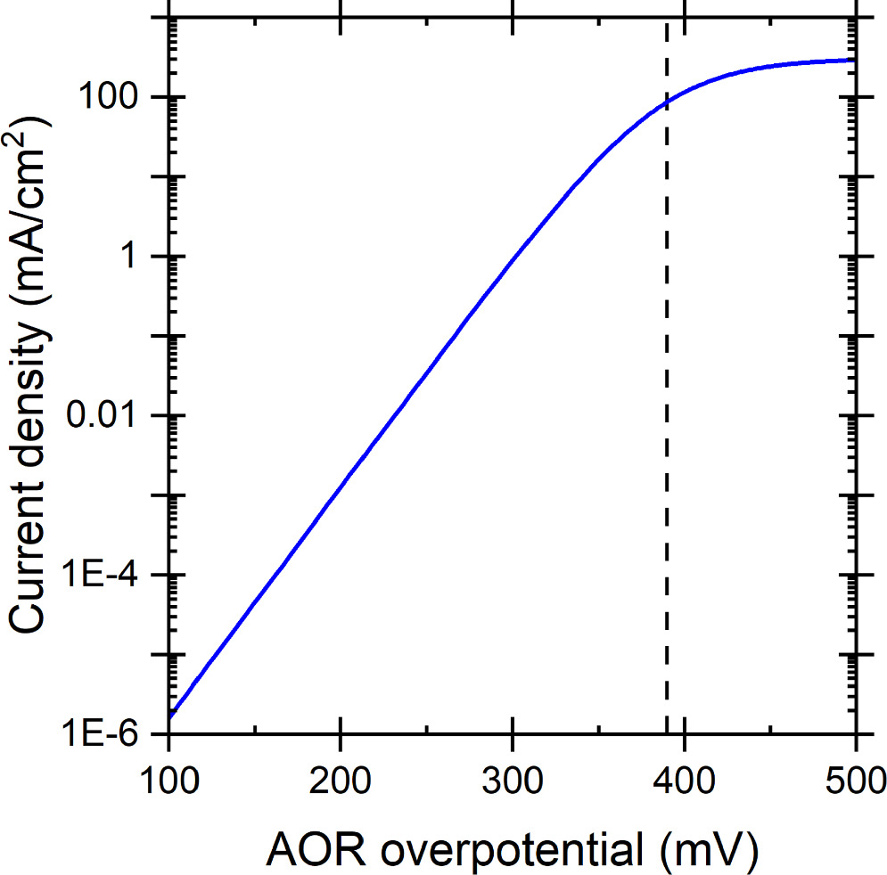
Figure 1. AOR kinetics at 75 °C modelled with the parameters that we used in our simulations. The vertical dashed line indicates the *NH2 potential  (389 mV overpotential).
Download figure:
Standard image High-resolution imageThe effect of temperature on the model parameters
While Zhao et al.
23
provided the necessary parameter values at 60 °C and at 95 °C, the temperature dependency was given for only some parameters. For kinetics ( and A), the Arrhenius equation was assumed, and a linear temperature dependency was shown for the *NH2 potential
  For the ORR, we used the given parameters directly. However, for the AOR we noticed that a numerical value given in a table (in supporting information, 35 A g−1 at 60 °C) did not quite match the kinetics data shown in the figures, most likely due to a typographical error, so we extracted the value and activation energy from the figure showing the catalytic activity parameter as a function of temperature (45 A g−1 at 60 °C and 33.89 kJ mol−1).
For the ORR, we use the theoretical voltage of water electrolysis together with the 0.9 V vs RHE potential to extrapolate the exchange current density of the ORR. A linear fit to the NIST-JANAF thermochemical tables 39 gave for the ORR
This corresponds also to the theoretical voltage of a hydrogen fuel cell (or a water electrolyser). A similar linear fit yields the theoretical AOR potential as follows

Therefore, the theoretical DAFC voltage as the potential difference of the half reactions is

A linear fit directly to the thermodynamic data of the total reaction yielded a temperature slope whose magnitude was about 2.5  V K−1 smaller, so we consider this difference negligible. The voltage and potentials are shown in Fig. 2, including also the *NH2 potential
  (Eq. 7).
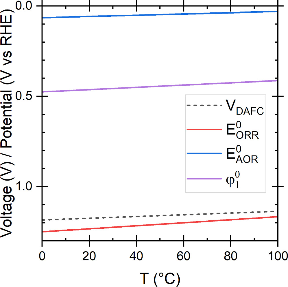
Figure 2 The theoretical potentials of the reactions and *NH2, and the theoretical voltage of a DAFC as a function of temperature.
Download figure:
Standard image High-resolution imageFor the ionic conductivity, based on the measurements of Schwämmlein et al., 40 we assumed that the product of conductivity and temperature follows the Arrhenius equation.

Fitting the values for the AEM and the catalyst layer conductivity yielded activation energies of 16.6 kJ mol−1 and 26.8 kJ mol−1, respectively. Also in this case, the reference temperature T0 is 95 °C.
The parameter values given by Zhao et al. 23 that we used are given in Table S1. For the AOR and ORR standard potentials we used Eqs. 8 and 9, and the ORR and AOR activities are assumed to follow the Arrhenius equation.
Comsol model
Using Comsol multiphysics (version 6.1), we constructed a one-dimensional (1D) macrohomogeneous cross-section model of the DAFC. In addition to the AEM and the CL, the model included the porous transport layers (PTL) between the CL and the gas channels. For comparison, we also considered single-layer electrodes composed of a homogeneous mixture of catalyst and ionomer in the pores of an electrically conductive substrate (that would be the PTL in case of a separate CL). Compared to existing cell architectures, these structures correspond to the catalyst-coated membrane (CCM) and catalyst-coated substrate (CCS), respectively, with their corresponding differences taken to their extremes. Schemes of the simulated layers (CCM: PTL and CL, CCS: CL) are shown in Fig. 3. The CCM electrodes have a clear CL between the AEM and the PTL, whereas in the case of the CCS the boundary between the CL and the PTL is more diffuse, and some of the catalyst can be deposited inside the PTL. 41 Depending on the amount, the model with a separate PTL and CL may be closer to an actual CCS structure than the single-layer model. The single-layer electrode model takes the catalyst deposition inside the PTL to its extreme and assumes uniform catalyst and ionomer loading throughout the porous electrode substrate. In practice, the catalyst and ionomer distributions would depend on the deposition method and other details but, for example, electrodeposition might allow for a more uniform distribution than most other methods. 42,43 For simplicity and differentiation, we call this the CCS, and such structure could correspond to e.g., a simplified picture of electrodeposited catalyst on a porous substrate with perfect ionomer infiltration. While the distribution might not always be uniform, we assumed this for simplicity and exclude the effect of the distributions from the scope of this study. Our model is limited to the effects of the catalyst and ionomer distribution in the electrode cross section, and thus cannot simulate e.g. the differences in the PTL-CL and CL-AEM interfaces of CCM and CCS 41 and their effects. It could be possible to imitate the differences in catalyst particle size and surface area 44 by varying the mass-specific catalytic activity accordingly, but all interfaces would require a more specific model.
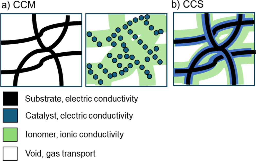
Figure 3 Schemes of (a) PTL and CL of a CCM and (b) CL of a CCS. The features are not to scale.
Download figure:
Standard image High-resolution imageAs mentioned, we assumed uniform catalyst loading in the catalyst-containing layers in all cases. With CCM, this meant constant loading per thickness, that the CL thickness depended linearly on the catalyst loading per geometric area. In the case of CCS, the layer thickness was fixed and the catalyst loading per volume depended linearly on the loading per geometric area. For the comparisons with the literature model we used PTL properties that corresponded to either typical carbon paper, or Sigracet SGL 29BC specifically, which was the carbon paper specified by Zhao et al. (in their SI). 23 In later simulations, because of our interest in using the material in DAFC, we used stainless steel felt (SSF) as the PTL or substrate. We continued using the catalyst parameters (activity, activation energy, *NH2 potential) in Table S1. To couple the ionic conductivity, water transport, and gas transport to the reaction kinetics and to each other, we needed to extend the models of the reaction kinetics, and of the ionomer and the AEM to account for these factors. To couple the reactions to gas transport, we added the effect of the oxygen partial pressure on the ORR kinetics and made both the AOR and the ORR reaction potentials and kinetics dependent on the partial pressures. The electrodes were composites of several materials, so we needed to model the effect of the electrode compositions and the base material properties. To be able to simulate the spatial distribution of e.g., ionic conductivity and its effect on the kinetic overpotentials, and the effect of relative humidity on them, we replaced the ionic conductivity of the catalyst layer and the AEM with a more detailed model of water uptake, water transport, and ionic conductivity. For gas transport, the relative humidity was set to be in equilibrium with the ionomer water uptake and the AOR and the ORR acted as gas sources or sinks.
General description and boundary conditions
Our model will be discussed in more detail in the following sections, and here we give a brief, general description of the cell operation together with a scheme of the cell cross-section, including the most important physical phenomena, couplings, and boundary conditions.
The most important physical phenomena are shown in Fig. 4 together with the associated boundary conditions. The CLs, where the electrochemical reactions occur, involve the largest number of phenomena and their interactions: Electric conductivity is needed to supply electrons to and extract them from the electrode, and hydroxide ions (and water) and gas need to be moved to and from the catalysts in the ionomer and empty space, respectively. The reactions, AOR and ORR, convert electric and ionic current to each other and couple the different forms of transport to each other. The AEM between the electrodes is responsible for connecting the reactions to each other through ionic transport, while blocking electron transport through the cell. In CCMs the gas that is transported into and out of the CLs proceeds through the PTLs, as well as the electron transport in the electrically conductive substrate (electric resistance, ohmic losses). As mentioned earlier, ammonia crossover through the AEM is not included in the model.
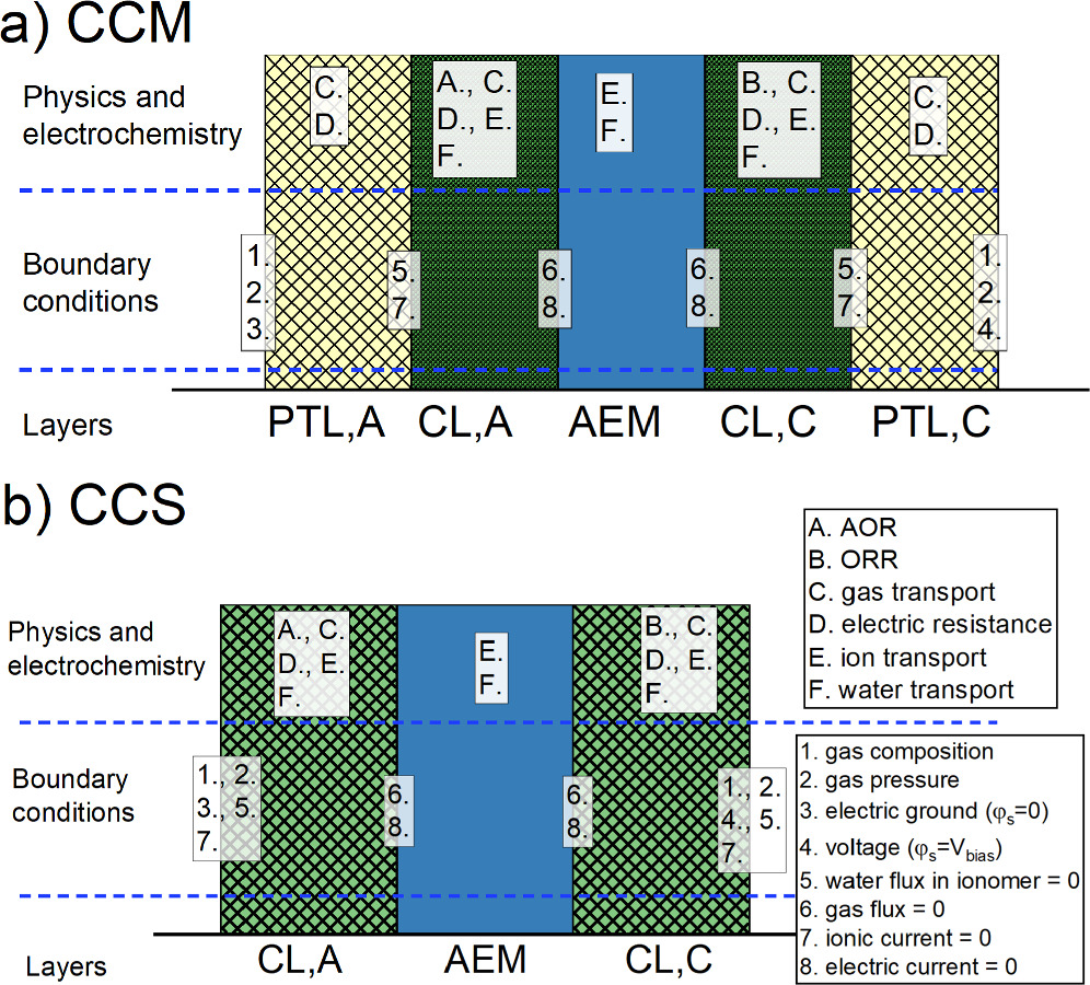
Figure 4 The general scheme of the most important modeled phenomena (letters) and their boundary conditions (numbers) for CCM (top) and CCS (bottom). The layer thicknesses are not to scale.
Download figure:
Standard image High-resolution imageElectrochemical kinetics
The contribution of the partial pressures was added to the theoretical AOR and ORR potentials using the Nernst equation


We assumed that water absorbed in the ionomer participated in the reaction, so the water activity was the ionomer water activity aw,m (defined later, Eq. 19), which was assumed to be in equilibrium with the gas phase humidity. The reference pressure for O2, N2 and NH3 is  The activity of the hydroxide ions in the ionomer and the AEM was assumed to be constant 1 and therefore it did not affect the potentials. The temperature-dependent reference potentials are given by Eqs. 8 and 9.
The main expression of the AOR kinetics is given by Eq. 5 and the effects of catalyst loading and gas transport amounted to varying the catalytic activity parameter A (or rather mcatalyst
A/L like in Eq. S2) and the ammonia concentration, respectively. Catalytic activity was assumed to depend linearly on the catalyst loading (per thickness or volume). The catalytic activity and the *NH2 reference potential  depended on temperature, as specified earlier in section "Literature model."
For the ORR, we extended the kinetics by assuming that the exchange current density depends on the square root of the O2 partial pressure, based on Neyerlin et al. 45

Here the reference pressure  corresponds to 3 bar absolute pressure, because Zhao et al. applied 2 bar gauge pressure to their cathode.
23
The local exchange current density depends on the catalyst loading and CL thickness (LCL), similarly to AOR and Eq. S2.
corresponds to 3 bar absolute pressure, because Zhao et al. applied 2 bar gauge pressure to their cathode.
23
The local exchange current density depends on the catalyst loading and CL thickness (LCL), similarly to AOR and Eq. S2.
Material volume fractions
We use effective medium approximation to describe the electrodes. For most properties, we used the Bruggeman approximation

The bulk property is marked with subscript b and the power 1.5 of the volume fraction  includes both the linear cross-section area reduction (
 ) and the consequently increased tortuosity that reduces e.g., ionic conductivity (
 ). However, with the ionomer volume, as discussed later in this section, the main parameter varied in simulations was the fraction of the empty volume left after the catalyst and substrate, and not the fraction of the total volume.
The solid volume fraction of both the SSF and the carbon paper substrates is 20%,  and in the CL of the CCM the carbon support of the catalyst occupies 25% of the volume,
  Carbon paper is based on ca. 2 g cm−3 solid density (amorphous carbon 1.8 − 2.1 g cm−346
), and on ca. 200
Carbon paper is based on ca. 2 g cm−3 solid density (amorphous carbon 1.8 − 2.1 g cm−346
), and on ca. 200  m thickness and 90 g m−2 areal weight
47
yielding 22.5% solid fraction, rounded down. The SSF properties are based on typical steel felt characteristics, e.g.
48
For the carbon support, using the anode properties of Zhao et al.
23
(4 mgPt cm−2 of PtIr, 340
m thickness and 90 g m−2 areal weight
47
yielding 22.5% solid fraction, rounded down. The SSF properties are based on typical steel felt characteristics, e.g.
48
For the carbon support, using the anode properties of Zhao et al.
23
(4 mgPt cm−2 of PtIr, 340  m thickness), 2 g cm−3 carbon density, and assuming that 20% of the total catalyst weight is metal, i.e. 80% carbon, yields ca. 24% carbon volume fraction. We rounded this up to 25% and assumed the same volume fraction for the cathode because a similar volume fraction could be produced with reasonable numbers. (At the cathode, 3 mg cm−2 of catalyst and 120 μm thickness with 30% of catalyst weight being metal would give a 29% carbon volume fraction. Without knowing the specific values, using 25% also for the cathode therefore seemed reasonable.)
When simulating the CCS, the catalyst has no additional support. The catalyst volume fraction depends on the layer thickness L, catalyst loading mcatalyst, and the density of the catalyst material 

For PtIr we use the average of the densities of Pt (21.4 g cm−3) and Ir (22.56 g cm−3), 21.98 g cm−3, and for the Acta 4020, an FeCo-based catalyst,
49
the density of cobalt iron alloy, 8.6 g cm−3.
50
As mentioned earlier, in the case of CCM, we assume that the catalyst loading per volume does not change, but the layer thickness depends on the loading, meaning that the catalyst volume fraction is constant (∼0.54% at anode and ∼2.9% at cathode, based on the catalyst loadings and layer thicknesses from Zhao et al.
23
), the baseline loading of 4 mg cm−2 of catalyst corresponding to a thickness of 340  at anode and to 120
  at cathode. In the case of the CCS and 0.5 mm thick SSF, the catalyst volume fraction depends on the catalyst loading, the baseline 4 mg cm−2 corresponding to ∼0.36% at anode and to ∼0.93% at cathode.
The electric conductivities of the substrate, catalyst, and possible carbon support were added together for the total electric conductivity of the layer. For the metals, we used their bulk values and the Bruggeman approximation, and in the case of the stainless steel felt we also considered the effect of the temperature. The conductivity of the carbon support was based on the data for carbon black from Pantea et al. 51
For the ionomer volume fraction, we vary the fraction of the non-solid volume ( ) in our simulations to ensure that that the sum of the volume fractions of all components is 1. The absolute ionomer volume fraction is

In practice, the absolute volume fraction is in most cases about 75–80% of the value of fε,ionomer. The remaining empty volume where gas is transported is
The main reason for this parameter choice was to simplify varying the parameter range by guaranteeing that the entire range from 0 to 1 would be feasible for fε,ionomer in all cases, meaning that the remaining empty volume fraction εvoid would always be positive.
Anion exchange membrane and ionomer
In this section we discuss our model for the AEM and ionomer, including the water uptake and transport, ionic conductivity and the ionomer volume fractions in the electrode layers.
The water uptake and ionic conductivity of the ionomer and the AEM are based on the parametrization given by Gerhardt et al. 52 and we only modify the ionic conductivity by reducing it by constant multipliers to match the values to the ones given by Zhao et al. 23 The water uptake is

In practice, we calculate the uptake from the water concentration (and ionomer density and equivalent weight, EW) and then solve the water activity using the formula for the cubic equation (see supporting information for details). 53 From the water volume fraction (f, Eq. 38 in Weber and Newman 54 ) the following expression for the water uptake can be derived, by recognizing that the water concentration is equal to the water volume fraction divided by the molar volume of liquid water (cW = f/VM,W)

The second term in the parentheses corresponds to membrane swelling, and the molar volume is equal to the molar mass divided by density, VM,W(T) = MH2O/ρH2O(T) (MH2O = 18.015 g/mol). For the density of liquid water, we used the data from the CRC Handbook of Chemistry and Physics. 46 For the EW we use 588.24 g mol−1 and the density is 1.1 g cm−3, both corresponding to Tokuyama A201 AEM. 52,55
The basis for the ionic conductivity, that we reduce by constant multipliers in both AEM and ionomer, is
The temperature is in Kelvins and the unit of the conductivity is S cm−1. In the catalyst layer, the effective conductivity is calculated using the Bruggeman model

To match the AEM of Zhao et al.
23
with  we divide the conductivity by 11.73, which is the average of the multipliers that match their measured values at 60 °C and at 95 °C (
 ). The match is of course not perfect because the temperature dependencies of this parametrized model and the reported values reported by Zhao et al.
23
differ from each other, but this model forms a good basis for simulating the effect of the DAFC operating conditions on the AEM and ionomer. For the ionomer, assuming
). The match is of course not perfect because the temperature dependencies of this parametrized model and the reported values reported by Zhao et al.
23
differ from each other, but this model forms a good basis for simulating the effect of the DAFC operating conditions on the AEM and ionomer. For the ionomer, assuming  (substrate volume fraction being
  and
and  i.e. ionomer occupying 85% of the non-solid volume), the best match at 95 °C would be achieved by dividing the conductivity by 5.23 and lower conductivities improve the match at lower temperature. For most of our simulations, we divided the ionomer conductivity by 7, because this value provided a close match near our 75 °C baseline temperature (as discussed later in "Results"). Here we are matching the product of two model parameters to one measured value, meaning in practice that one parameter needs to be fixed (ionomer volume) before the other (conductivity) is varied for the best fit. If the resulting layer conductivity does not change, the individual parameters values are not important for most of the ionomer volume fraction range (discussed later in "Results—Ionomer Volume Fraction and Gas Transport").
We model the water flux in the ionomer as a sum of the diffusional flux and the electro-osmotic drag. However, due to software limitations, we needed to adapt the electro-osmotic drag term to a form of drift in electric field, which we explain in this section. In steady state

And the water flux is

The bulk diffusion coefficient is the parameterization given by Gerhardt et al. 52 without the term for the fraction of the bicarbonate form of the ionomer, and in the ionomer we apply the Bruggeman model to account for the ionomer volume fraction.

As mentioned, the water activity is solved as the inverse of Eq. 19.
The electro-osmotic drag of the water molecules in the ionomer and AEM is included in our model. We assume that the hydroxide ions drag water molecules in the same direction with them and that the fluxes are equal to each other. 52,56


The ionomer/AEM conductivity ( ) is the conductivity determined by the cell temperature and water activity. In practice, we implement this using the "Migration in electric field" option in the Transport of Diluted Species node of Comsol. The electronic/ionic current is driven by the electrolyte potential gradient (
 ), so, for the water flux to match the hydroxide, the water mobility (
 ) needs to be expressed as a function of the ionic conductivity and water concentration.

From this and Eq. 28, an expression for the mobility follows, setting  and
and  (Eq. 21)

This is treated as a variable, meaning that the value is calculated for each point in the cross-section with the corresponding water uptake and ionomer conductivity. In the catalyst layers both the ionic current density (conductivity) and water mobility are corrected with the volume fraction of the ionomer according to the Bruggeman model

Both AOR and ORR are assumed to produce or consume water, respectively, in the ionomer, corresponding to a source term

The current density iV is the reaction rate per volume, in A m−3, and the source term thus has the dimension mol m−3. For AOR, the number of electrons is  and the stoichiometric coefficient
  and for the ORR,
  and
and  (see reactions (2) and (3)). In fuel cell operation the current density of the AOR is positive (oxidation), hence this source term is also positive, corresponding to water generation. For the ORR, the opposite applies.
The water activities in the ionomer and in the gas are assumed to be in equilibrium, which we in practice enforce with a kinetic source term with a high rate constant

For the rate constant we use 106 mol m−3 s−1 as a large value to enforce equilibrium of water activities in the ionomer and in the gas. Negative values correspond to water evaporating from the ionomer to the gas and positive to the ionomer absorbing humidity from the gas. We assume that the gas phase activity is equal to the relative humidity, the ratio of the water partial pressure to the vapor pressure.

Gas transport
We calculate the flow of the gas mixture in the porous layers using Darcy's law, meaning that the gas velocity ( ) depends on the pressure gradient, dynamic viscosity of the gas (
 ) and the permeability (
 ) of the porous layer.


The density of the gas is  and Qm is the mass source. The density
  and dynamic viscosity
  (subscript v to differentiate from ionic mobility) depend on the gas composition as will be defined later in this section.
For the permeability of the carbon paper we used the value  based on Mangal et al.
57
We calculated the permeability of the SSF using the Carman-Kozeny equation
based on Mangal et al.
57
We calculated the permeability of the SSF using the Carman-Kozeny equation

We used the value for a fibrous medium,  58
for the geometry constant and 10
58
for the geometry constant and 10  m as the fibre diameter (d). In all layers, the void volume fraction was calculated with Eq. 18.
At the CL-AEM boundaries we set a no flow boundary condition for the gas mixture and fixed the pressure at the PTL-gas channel boundary to the total absolute pressure. This is the sum of the pressure of dry gas (N2, O2, NH3) and the water pressure that corresponds to the set relative humidity at the cell temperature. The water partial pressure is calculated as the product of the RH and the vapor pressure given by Eq. S8.

The dry component consists of NH3 and N2 at the anode, and of O2 and N2 at the cathode. For both the anode and the cathode gas inflow, we define the molar fractions of these molecules as

For the dynamic viscosity and binary diffusion coefficient we used Comsol's built-in values and models, selecting the Fuller-Schettler-Giddings model for the gas diffusivity and Wilke's model (without high pressure correction) for the gas viscosity. Wilke's model for the viscosity of a multi component system is 59,60


The mole fractions xk depend on the diffusion of the species in the mixture, as discussed below. The vapor phase viscosity coefficients of all species ( ) were set by Comsol Multiphysics and depend on the temperature. While not the precise expression used by Comsol, in our temperature range (20–95 °C) the viscosity coefficients increasing as T0.76 is a reasonable approximation of the values used in the simulations (temperatures in Kelvins)

The values at the 75 °C baseline temperature are given in Table S3. We modeled the mixture as ideal gas so they were independent of the cell pressure.
The density and viscosity of the gas were calculated from the gas composition and the diffusion of the molecules in the gas mixture was calculated using Maxwell-Stefan diffusion 61 in the Transport of Concentrated Species node.

The average velocity of the gas mixture is  and its density is
  The mass fraction, mass source and mass flux of species i relative to the average velocity are
  Ri and
  respectively. The mass flux, neglecting thermal diffusion, is
60
respectively. The mass flux, neglecting thermal diffusion, is
60

Here  are the multicomponent Fick's diffusion coefficients. Without external forces acting on the gas mixture and in the presence of total and partial pressure gradients, the diffusional driving force acting on species k,
  (unit m−1) is
60
(unit m−1) is
60

Here pA
is the total absolute pressure (see Eq. 38), xk the mole fraction and  the mass fraction of species k.

Here Mk and Mn are the molar mass of species k and the effective molar mass of the mixture, respectively,

We assumed ideal gas, so the density was calculated from the molar masses (Mk) and mass fractions of the species

The binary diffusion coefficients of the molecules were calculated using the Fuller-Schettler-Giddings model. 60,62

Here the temperature is in Kelvins, pressure in Pa, molar masses MA and MB in g mol−1 and the resulting diffusion coefficient is in cm2 s−1. Similarly to the other transport processes described in the previous sections, the Bruggeman model was applied to the gas diffusion.

For the definition of the void volume fraction, see Eq. 18.
The values of the molar volumes  used by Comsol to calculate the total molecular volume are given in Table S3.
60,63
In general, the total volume of a molecule is based on the contribution of the contained groups summed together, but in our case the diffusion volumes of the molecules have specific values (that are different from the sum of the diffusion volume increments of the composite atoms).
used by Comsol to calculate the total molecular volume are given in Table S3.
60,63
In general, the total volume of a molecule is based on the contribution of the contained groups summed together, but in our case the diffusion volumes of the molecules have specific values (that are different from the sum of the diffusion volume increments of the composite atoms).
At the PTL-gas channel boundary, we set a flux boundary condition for all species of the gas mixture that corresponded to the difference of the selected gas inflow composition and the true molar fractions.

The volumetric gas inflow rate per electrode area is Q (which has the dimension of velocity, e.g. ml min−1 cm−2 = cm min−1), Mk is the molar mass of species k, Mn is the effective molar mass defined in Eq. 47 and xk and xk,in are the mole fractions of species k at the boundary and in the specified gas mixture flowing into the DAFC, respectively. Positive values correspond to more of species k flowing into the PTL and negative to the species flux being out of the electrode. The dry molar fractions fk (that we used as a varied parameter in our study) and the total inflow mole fractions xk,in differ from each other by a factor that depends on the RH and the absolute dry pressure.

Sensitivity analysis
We study the effect of the operating conditions and cell parameters on the DAFC performance by varying each parameter individually, while keeping the rest fixed to their baseline values. To estimate their relative importance, we change the parameters in each case by 20% of the baseline value (in case of temperature 20% of the value in degrees Celsius), which was selected so that all 20% variations would be within the physically realistic range. The parameter list as well as the values for the comparison to Zhao et al. 23 and for the baseline and the 20% range of the sensitivity analysis are shown in Table I. The cell is assumed to be at uniform temperature, so different from the other parameters, the separate contributions of changes to the anode and cathode side were not evaluated. The gauge pressures are dry pressures and the total absolute pressure is the sum of the absolute dry pressure and the water vapor pressure, given by the RH and temperature (Eqs. 34 and 38). We simulated a wider value range for all parameters shown in the table, but this range was chosen to compare the importance of the parameters with each other, and in the most important cases, we discuss also the effects over a wider parameter value range. The catalyst loadings and gas flow rates were set equal at the anode and at the cathode for simplicity. The cathode flow rate 100 ml min−1 cm−2 was selected as the baseline simply because it was a round number, and the higher anode catalyst loading was selected to avoid reducing the cell performance too much by increasing the AOR kinetic overpotential. The dry fraction of O2 at the cathode had to be reduced from 99% (not 100% to avoid numerical issues with 0% N2 fraction) for the 20% increase to be physically feasible, so we chose to set the reduced fraction to be equal to the anode NH3 dry fraction.
Table I. Operating conditions and cell parameters studied in the sensitivity analysis.
| Parameter, (unit), [symbol] | Literature comparison | Baseline [and range] in the sensitivity analysis |
|---|---|---|
| Temperature (°C) [T] | 60–95 | 75 [60–90] |
| Relative humidity [RH] | 1 | 0.75 [0.6–0.9] |
| Anode AOR activity (A g−1) [A] | 45–144 | 76.2 [61.0–91.5] |
| Cathode ORR activity at 0.9 V vs RHE (A g−1) [i0] | 7.1–10 | 8.3 [6.6–9.9] |
| Anode catalyst loading (mg cm−2) [mcatalyst,A] | 4 | 4 [3.2–4.8] |
| Cathode catalyst loading (mg cm−2) [mcatalyst,C] | 3 | 4 [3.2–4.8] |
| Anode (dry) gauge pressure (bar) [pg,A] | 0 | 1 [0.8–1.2] |
| Cathode (dry) gauge pressure (bar) [pg,C] | 2 | 1 [0.8–1.2] |
Ionomer volume fraction [ ] ] | 0.85 | 0.75 [0.6–0.9] |
| Anode gas flow rate (ml min−1 cm−2)) [QA] | 160 | 100 [80–120] |
| Cathode gas flow rate (ml min−1 cm−2)) [QC] | 100 | 100 [80–120] |
Anode NH3 molar fraction [ ] ] | 0.5 | 0.5 [0.4–0.6] |
Cathode O2 molar fraction [ ] ] | 0.99 | 0.5 [0.4–0.6] |
The voltage loss over the AEM is calculated simply as the electrolyte potential difference between the electrode-AEM interfaces at the anode and the cathode sides. All other overpotentials are averages, based on the total power loss due to the process in question

This is integrated over the thickness of the related electrode and the current source iV has the dimension of A m−3. The geometric current density iA (A m−2 or more commonly mA cm−2) is simply the volumetric source integrated over the electrode thickness, which is equal to the electric current density out of the anode

Results
We begin by validating our model against both the experimental results and model of Zhao et al. 23 This is followed by the general discussion about the sensitivity to the operating conditions and cell parameters, and we also discuss the effects of RH and gas flow, catalyst loading, gas composition, and gas pressure in more detail. Finally, we comment on the differences of simultaneous changes to several parameters compared to the changes to one parameter at a time. Because of the choice of the baseline parameters discussed earlier, the baseline DAFC performance is naturally suboptimal. Therefore, the baseline power should not be taken as our estimate of what the AEM DAFC technology is capable of because realistic changes to any parameter would increase the maximum power. As mentioned previously, our main goal is to evaluate the relative importance of the cell parameters and operating conditions, thus some conscious simplifications and downgrades were made to the baseline parameters.
Validation by literature comparison
We verified the 1D Comsol transport model described earlier by comparing it against our calculations using the model developed by Zhao et al.
23
(section "Literature model" and SI). The comparison to their experimental measurements and to their model is shown in Fig. 5. The DAFC performance at high current densities is underestimated by both simulations because, at over 70 °C temperatures, the AOR parametrization of Zhao et al.
23
overestimates the kinetic overpotentials at high current densities. The open circuit voltages match well so the effect of ammonia crossover appears small, which would be in line with the reduction to the crossover rate that they observed with gaseous anode feed compared to liquid feed. For the comparison with their experiments and model, we set the ionomer volume fraction ( in Eq. 17) to 0.85 (corresponding to about 0.65 absolute volume fraction) and divided the ionomer conductivity by a factor of 5.23 because these values match the specified catalyst layer conductivity at 95 °C temperature. (We used different values for all other simulations due to different baseline temperature, as discussed below.) The ionomer volume fraction effects will be discussed in more detail in a following section but, in short, our choice was to essentially match a very good but not quite optimal (according to our model) CL composition. At 95 °C the simulations match each other, the voltage difference at current densities below the maximum power being less than 5% (Fig. S2), and the measurements. However, at lower temperatures the Comsol model overestimates the DAFC performance due to the different temperature dependencies of the ionic conductivity.
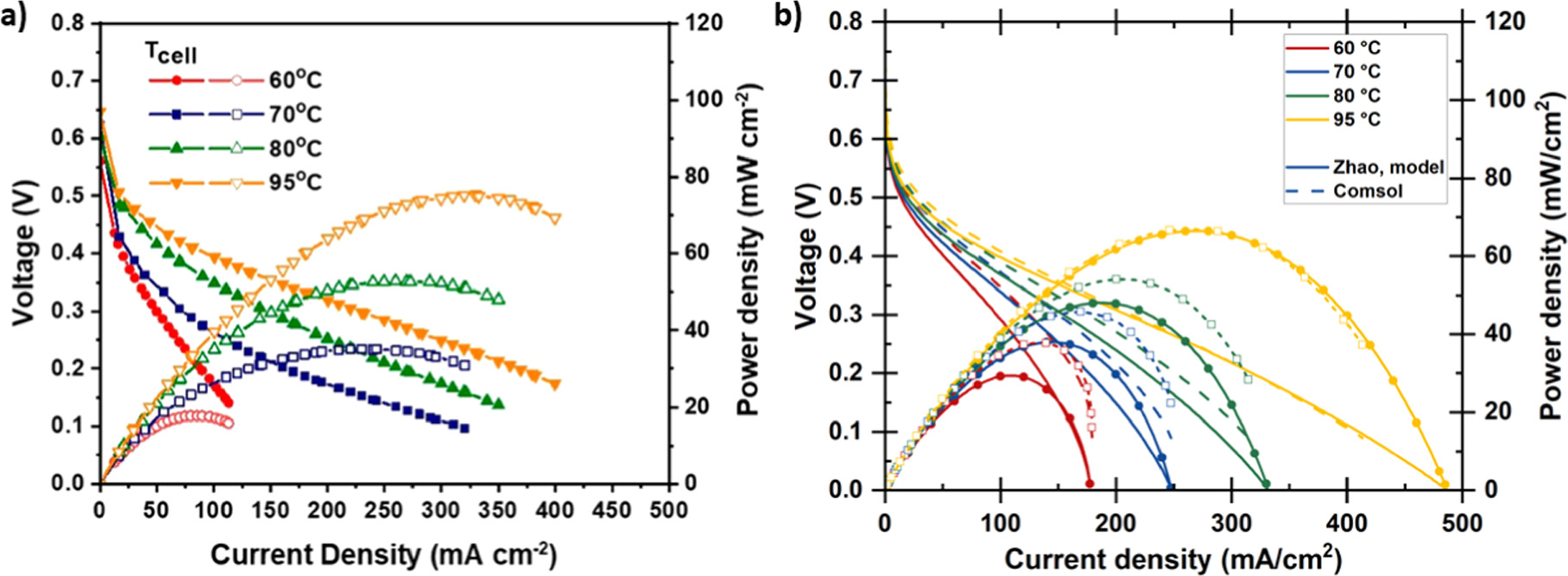
Figure 5 (a) Experimental DAFC voltage and power density vs current density. Reprinted with permission from. 23 Copyright 2021 American Chemical Society. (b) Simulations with the literature model (solid lines and round markers) and with our Comsol model with ionomer conductivity reduced by a factor of 5.23 (dashed lines and open squares).
Download figure:
Standard image High-resolution imageFor a better match at our 75 °C baseline temperature, and therefore for all later simulations, we selected ionomer conductivity that would match the literature model at this temperature. In practice, we simulated the DAFC operation with different ionomer conductivities and dividing the value given by Eq. 21 by 7 gave the best match at 75 °C (Fig. S1), so we chose it for our study (instead of 5.23, AEM conductivity was not changed!). The effect of temperature on the DAFC performance is reduced compared to the properties of the ionomer that Zhao et al. 23 used but, although our model will not provide an exact picture of their DAFC, it should still provide a good estimate of the operation of a DAFC. The ionomer volume fraction is higher than what is common in literature, which may in part be due to our comparatively low current densities (especially in comparison to HFCs). As lower reactant supply and product removal rates are sufficient, gas transport does not need to occupy as large volume to satisfy these requirements so the optimal composition could favor lower gas volume and higher ionomer volume for reduced ion transport losses.
Sensitivity to the operating conditions and cell parameters
The largest voltage loss components were the AOR and ORR kinetics, followed by the ionic transport losses at the anode, and then the transport losses in the AEM and in the cathode which were roughly equal, but the AEM losses were lower at low current densities and increased faster. This was the same for both the CCM and the CCS, although in the latter case, the losses were generally larger and current densities slightly lower, as shown in Figs. 6 and S3. The ca. 300–350 mV ORR losses and the small AEM and cathode ionomer losses approximately match the results of Singh et al. 64 for AEM-HFC at low current densities (below 100 mA cm−2) and the voltage breakdown of Gerhardt et al. 52 The somewhat lower ORR losses of Singh et al. 64 are likely explained by different ORR catalyst. Gerhardt et al. 52 studied the effect of along channel transport effects on AEM HFC at 60 °C temperature, so all voltage losses naturally depend on the position along the channel, and the temperature is lower than ours. Nevertheless, their ORR losses did not vary much and were similar to ours, and the ionomer losses were significantly smaller than the ORR losses. The AEM losses, and anode and cathode RHs depended on the position along the channel, so accurate comparison is very difficult, but the AEM losses were approximately equal to the cathode ionomer losses right before anode RH saturation to 100% (cathode RH ca. 60% at that point). Additionally, in our simulations there were smaller losses due to mass transport, or concentration polarization, and ohmic losses due to electric current flow at both electrodes, but these were negligible compared to the losses shown in Fig. 6. (Concentration polarization losses are implicitly included as the not-quite-horizontal top of the AOR kinetics region.) Especially the anode losses increased with increasing current density (see Fig. S3) and dominate the DAFC performance, as expected based on literature data on AOR kinetics 65,66 and on comparisons with H2 as the anode fuel, 27 and the original calculations of Zhao et al. 23 In both cases the maximum power density is achieved at 0.27 V, but for later comparisons we select the 0.25 V as an almost round number and because the power difference between the voltages was minimal. The current densities at 0.25 V were 93.2 mA cm−2 and 76.0 mA cm−2 with CCM and CCS, respectively, corresponding to 23.3 mW cm−2 and 19.0 mW cm−2 power densities.

Figure 6 The voltage loss breakdown for the baseline scenario with (a) CCM and (b) CCS. The dashed lines indicate the comparison point at 0.25 V. The top of the coloured region, indicating the thermodynamic voltage, is not perfectly horizontal due to mass transport losses (i.e., concentration polarization), but these are negligible compared to the indicated losses.
Download figure:
Standard image High-resolution imageThe effect of the parameters listed in Table I on the power at 0.25 V is shown in Fig. 7. Figure (a) shows the effect with a CCM and (b) with a CCS, both using SSF as the PTL or the electrode substrate. The baseline power was 4.3 mW cm−2 higher with the CCM than with the CCS. In terms of absolute power increase or decrease, both electrode constructions are generally similar, although there are differences. Overall, the most significant parameters were relative humidity (RH), cell temperature, and (anode side) ionomer volume fraction, all of which have a direct effect on at least one of the two main losses: reaction kinetics or ionic conductance of the electrodes (especially anode). These parameters are commonly studied in AEM-HFC modeling and simulation studies, such as, 35,67,68 indicating their significance. Regarding their importance compared to each other, the higher sensitivity to RH than to temperature is similar to Jiao et al. 67 who simulated AEM-HFC operation, and the roughly similar sensitivity to RH and ionomer content of the catalyst layer is similar to Dekel et al. 35 at low current densities. These parameters are also among the most important for PEM-HFC operation. 69
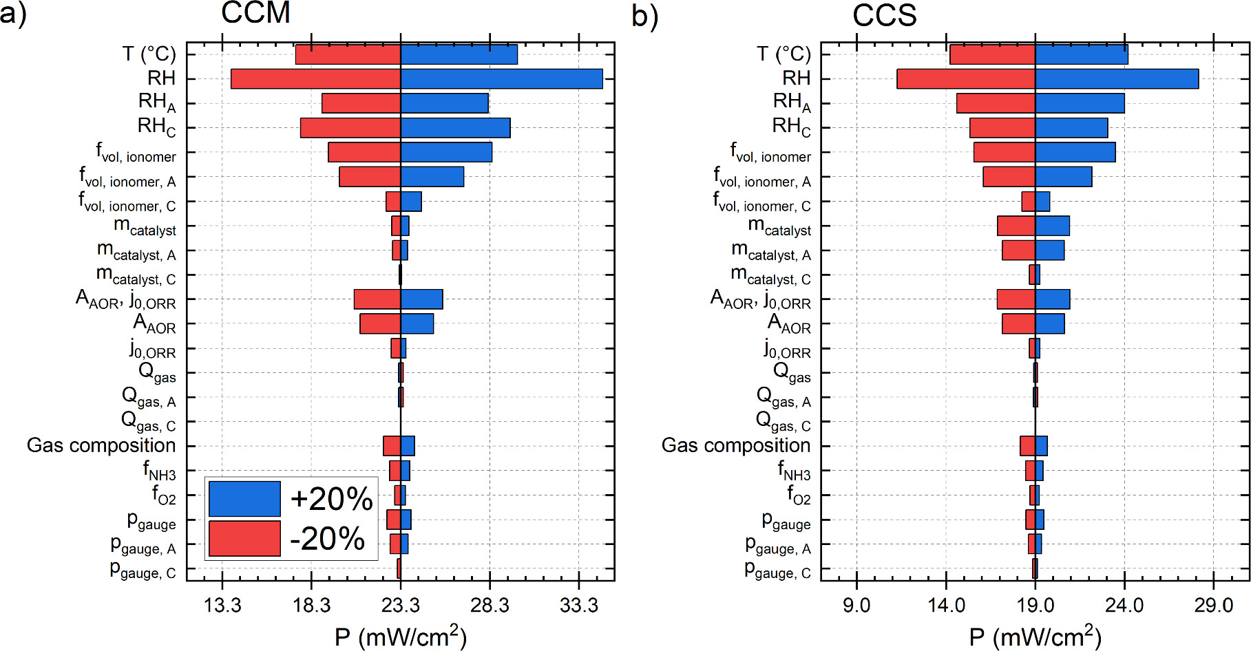
Figure 7. The effect of the selected operating and cell parameters on the DAFC power at 0.25 V for (a) CCM and (b) CCS. In both figures the blue and red bars indicate the effect of increasing and decreasing, respectively, the parameter in question. Where anode (A) or cathode (C) is not specified, the effect corresponds to the simultaneous increase or decrease of the property in question at both electrodes.
Download figure:
Standard image High-resolution imageOf course, in our case, the sluggishness of the AOR compared to the HOR makes the anode kinetics a more significant factor than it is for HFCs and, with the CCS, also the anode catalyst loading has a noticeable effect on the power. Surprisingly, with the CCM, changing the catalyst loading had only a very minor effect on the power. However, when directly varying the catalyst activity (A or j0), both structures responded very similarly to the effect of catalyst loading on the CCS. This we will discuss in more detail later. Also, increasing the gas flow rate decreased the power a little, which we will discuss together with the gas composition effects. The effect of the pressure was one of the smallest, due to the magnitude of the change, but it could still be as important as RH or temperature for the DAFC performance, which we also discuss.
Following this general look at the effects of the parameters, we discuss the parameters with the largest impact on the DAFC power in the following sections. We also describe the most significant differences between the CCM and the CCS, and few related parameters in more detail, as well as the combined effect of all studied parameters. In addition to the 0.25 V voltage (for power density comparisons), we also use selected current densities for voltage loss comparisons, i.e., 75 mA cm−2 when possible and 50 mA cm−2 when some parameter combinations did not achieve 75 mA cm−2. The simulations were carried out for cell voltages in 20 mV steps (from 0.91 V to 0.09 V) and the data for the selected current densities is interpolated from the voltage-based data.
Ionomer volume fraction and gas transport
The catalyst layers need to balance electron and ionic conduction with gas (and water) transport. Increasing the volume fraction of any conducting material (for gas transport, the empty space) increases the losses associated with the other two processes by reducing the associated conductance (following Eq. 15). From preliminary simulations, we already knew that the optimal ionomer volume fraction ( ) in our model would be over 0.9 (corresponding to about 0.7 absolute volume fraction, Eq. 17). For the literature comparison, we chose to use slightly lower volume fraction to represent a very good, but perhaps not fully optimized catalyst layer. In the case of the sensitivity study, the baseline value had to be lower than 0.83 to enable a 20% increase. To avoid constricting the performance by limiting gas transport, and to match the temperature and RH, we chose the slightly lower 0.75 volume fraction (ca. 0.55–0.60 fraction of the total volume, depending on substrate, catalyst loading etc, Eq. 17). When varying the ionomer volume fraction and conductivity together so that the resulting layer resistance is constant, the ionomer volume has only a small effect on the DAFC polarization curve, except at high volumes (ca. 0.9 or more) where anode RH is first increased, increasing conductivity and improving performance (Fig. S5), and further increase would begin to limit reactant transport reducing the power.
The effect of the ionomer volume fraction on the DAFC power density at 0.25 V voltage is shown in Fig. 8. The maximum powers are ca. 30 mW cm−2 for the CCM and ca. 24 mW cm−2 for the CCS. The effects of the ionomer volume are very similar for both electrode types, and the power is more sensitive to the anode than to the cathode volume fraction. At very high volume fractions, the power is reduced because constricted gas transport decreases the Nernst voltage of the cell and increases both the kinetics and ion transport losses in the electrode, as illustrated in Figs. 9 and S4. Importantly for the cell and electrode optimization, the volume fraction of the highest power depends on the electrode structure. With the CCM, the optimal volume fractions are ca. 0.95 at both electrodes, whereas in the case of the CCS the peak is at around 0.9 for both electrodes. Because the transport at the level of microstructure is not included in our model, the total mass transport losses are likely underestimated (see e.g. 70 ) and therefore the optimal ionomer volume fractions overestimated. Additionally, our relatively low current densities likely also bias the optimum towards high ionomer volume fractions, as higher current densities would require faster gas transport, i.e. lower ionomer volume fraction. Therefore, the optimal absolute numbers are probably not very important, but the main results are the differences in anode vs cathode and CCM vs CCS comparisons. In the case of CCS, the lower optimal volume fractions are likely due to the entire 0.5 mm electrode thickness becoming more constricted, whereas with CCM the affected CL thickness was 0.16 mm (cathode) or 0.34 mm (anode). The generally higher sensitivity to the anode volume fraction is likely due to the higher anode overpotentials and higher sensitivity to the ammonia concentration than to the oxygen concentration (discussed later).

Figure 8. The effect of the ionomer volume fraction (fraction of volume left after catalyst and substrate) on the power density at 0.25 V voltage (a) CCM (b) CCS.
Download figure:
Standard image High-resolution image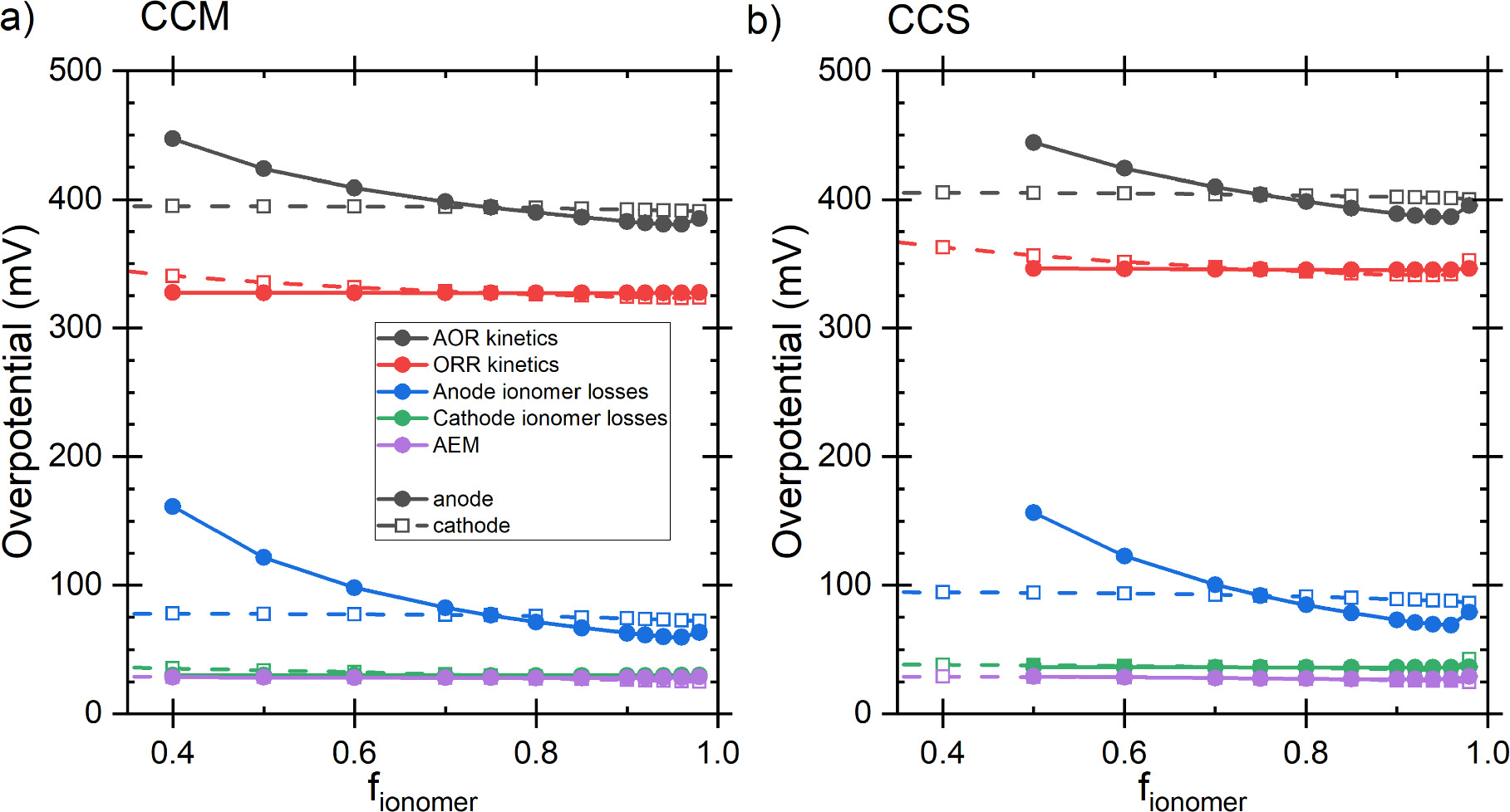
Figure 9. The effect of either the cathode and anode ionomer volume fractions, with that at the other electrode fixed at 0.75, for (a) CCM and (b) CCS. Solid lines and round markers correspond to anode properties being varied and dashed lines with open squared to the cathode properties being varied. Below 0.4 (a) or 0.5 (b) anode volume fraction the DAFC did not achieve 75 mA cm−2, hence the missing points and more limited range than in Fig. 8.
Download figure:
Standard image High-resolution imageThe voltage losses as a function of the cathode and anode ionomer volume fractions at 75 mA cm−2 current density are shown in Fig. 9. In this figure, and in the other similar figures, the solid lines and round markers correspond to the anode properties being varied and the dashed lines with open squares to the cathode properties being varied. Up to about 0.95 both the kinetic and ionic transport losses of the varied electrode decrease, but increase with further ionomer volume increase, especially at the anode, as the reduced reactant supply and product accumulation begin to slow the kinetics and even move the reaction farther from the AEM. The higher sensitivity of the anode side losses, and the increase at the highest volume fractions explains the pattern seen in Fig. 8. The thermodynamic voltage of the DAFC decreased with increasing volume fractions, except in the case of the cathode volume fraction of the CCM. The biggest effect came from the concentration polarization at the varied electrode, the CCM cathode being less sensitive than the other electrodes (CCM ca. 8.6 mV vs ca. 1 mV, CCS ca. 13 mV both), and most of the difference between the lowest and highest volume fractions came from the difference between the two highest simulated volume fractions (supporting information).
We assumed that each layer is a homogeneous mixture of the component materials and, as mentioned, neglected transport at smaller length scales. Considering the transport at different length scales would affect the transport in the ionomer-catalyst mixture, especially at high ionomer volume fractions, when considering that (more of) the catalysts would become deeper embedded in the ionomer, or the catalyst particles could become poorly connected with each other increasing electric resistance especially in CCM. This could add further restrictions that would begin to limit the DAFC operation at lower ionomer fractions but, at roughly equal ionic conductivities at anode and at cathode, and with the AOR maximum rate fixed to the rate A, the DAFC would likely remain more sensitive to the anode properties than to the cathode properties. While the optimal ionomer loadings could be lower than indicated here, in a CCS they could be somewhat lower than in a CCM due to the affected layer thicknesses. Additionally, the optimal ionomer loadings could in principle depend on the catalyst activities, but there are several qualifiers related to this statement. Higher activities enable higher current densities, which would require higher mass transport rates, so gas transport could then need more open electrode structures. Compared to HFCs, the optimal DAFC electrodes could therefore have slightly higher ionomer loadings and more closed structure, assuming that this does not negatively impact the electrocatalytic performance. This is of course temporary, until the DAFC current densities reach levels comparable to HFCs, neglecting the possible effect of different reactant gases, and it might not make sense to fully optimize a device for significantly lower performance levels than what is targeted.
Reaction kinetics and catalyst loading
The effect of catalyst loading on the power density at 0.25 V voltage is shown in Fig. 10. As shown earlier, at the baseline 4 mg cm−2 loading the CCM achieves a higher power than the CCS, but the CCS is more sensitive to the catalyst loading and achieves significantly higher power densities at high catalyst loadings. The main reason for this is the anode ion transport overpotential. While the kinetic losses were reduced by increased catalyst loading, the increase in ion transport losses reduced the total gains, similarly to the results of Singh et al. about AEM-HFC cathode. 64 Although Hu et al. 28 found experimentally the optimal DAFC cathode catalyst loading to be only 2 mg cm−2, the relatively low effect of the catalyst loading compared to other varied parameters is similar to our results. Similar behavior has been observed also in PEM-HFC simulations. 71 The effect of the catalyst loadings on the voltage losses at 75 mA cm−2 current density is shown in Fig. 11. The CCS anode differs from the other three electrodes in that increasing the catalyst loading decreases both the kinetic and the ionic transport losses in the electrode, explaining its higher sensitivity. The behavior of the other three electrodes was more similar to each other, albeit the changes in the overpotentials were different in their magnitude: with increased catalyst loading the kinetic overpotential was reduced and the transport losses barely changed, and the kinetic overpotential of the other electrode (constant 4 mg cm−2 loading) remained constant. As an exception, in the case of CCM, increasing catalyst loading increased the ionomer losses at catalyst loadings below 3 mg cm−2 (Fig. 11a).
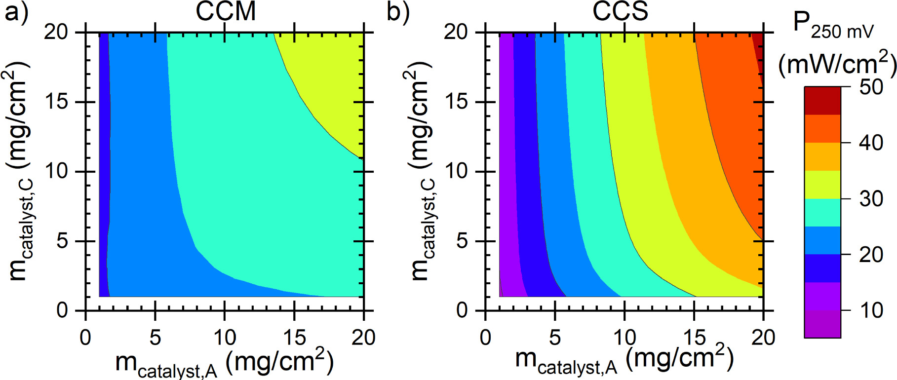
Figure 10. Power density at 0.25 V as a function of the catalyst loading for (a) CCM and (b) CCS. The baseline scenario corresponded to 4 mg cm−2 loading at both electrodes.
Download figure:
Standard image High-resolution image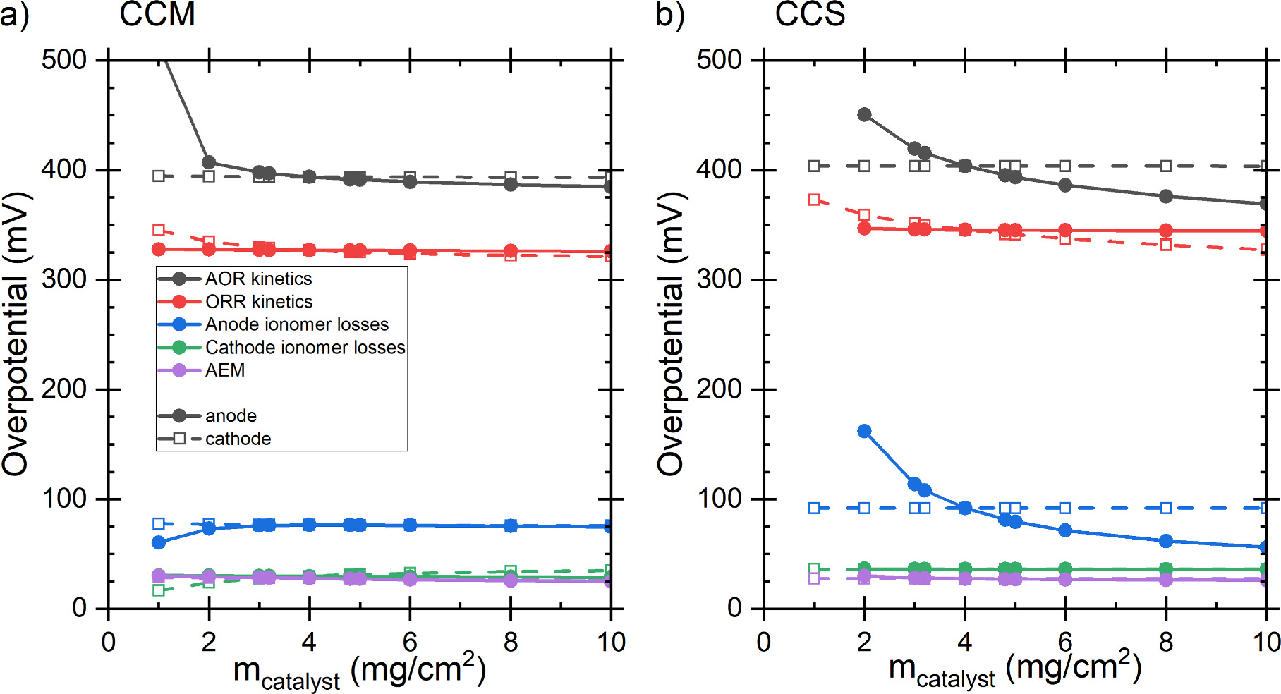
Figure 11. Voltage losses at 75 mA cm−2 current density as a function of the catalyst loading with (a) CCM and (b) CCS. The baseline loading was 4 mg cm−2. Solid markers and lines correspond to changing the anode PtIr loading with 4 mg cm−2 cathode loading and open markers and dashed lines to varying the cathode catalyst loading with 4 mg cm−2 anode loading. In figure (b) 1 mg cm−2 achieved only ca. 55 mA cm−2 current density, hence there is no data for 75 mA cm−2.
Download figure:
Standard image High-resolution imageAs discussed in the model description, with CCM we assumed that increasing the catalyst loading increases the catalyst layer thickness linearly (constant catalyst volume fraction), whereas with the CCS increased loading corresponds to more catalyst in the same thickness. Therefore, especially with the maximum rate limitation of the AOR kinetics (Eq. 5), increasing the catalyst loading per electrode thickness increases the rate near the AEM, bringing the reaction closer to it, thus reducing the ionic transport distance and losses. In the case of the CCS cathode, i.e., Butler-Volmer kinetics, the ionic transport losses in the electrode are not appreciably affected by the catalyst loading. Therefore, we ascribe the sensitivity of the CCS anode to the mathematical form of the AOR kinetics, i.e., the RDS not being electrochemical by nature.
With both electrode types, varying the catalyst activity produces results that are very similar to the effect of the catalyst load on the CCS: At constant 75 mA cm−2 current density, the kinetic overpotential of the varied catalyst responds expectedly, with almost all other losses remaining constant, as shown in Fig. S6. However, the anode ionomer losses decrease with increasing anode activity, due to the mathematical form of the AOR kinetics and the eventual saturation to A. Compared to varying the catalyst loading and to the baseline scenario, the relative range is wider, but nevertheless the CCM anode shows clear differences in the response of the ionic transport losses: ionic transport losses increase with increased catalyst loading (i.e. CL thickness), but reduce with increased catalyst activity. In contrast, for the CCS, the responses to catalyst loading and activity are similar because the catalyst loading only affects the catalyst volume fraction which is small (and thus indirectly the absolute ionomer volume) but does not affect the layer thickness.
Increasing the anode loading with CCM expectedly decreased the AOR kinetic losses and, interestingly, increasing the cathode loading also reduced the AOR kinetic losses, which was clearest at over 10 mg cm−2 anode loadings (Fig. S7). Although the effect was smaller, the same happened to the ORR kinetics at high cathode catalyst loadings when increasing the anode loading. In both cases the difference was visible only at over ca. 50 mA cm−2. With CCS this effect was practically absent (Fig. S8). The practical effect is quite small, especially at lower catalyst loadings, but this demonstrates that the electrode kinetics and transport losses are not fully independent of each other and for the best accuracy this should be considered. In principle, cell optimization therefore should not be done one electrode at a time, independent of the other, but the effect on practical device optimization is probably negligible.
The enhancement of the unchanged electrode was due to water transport. Increasing the CCM catalyst loading increases the electrode thickness, which then increases the RH and ionomer (and AEM) conductivity in the cell, reducing ionic transport losses. This in turn slightly increases the reaction rate throughout the CL at constant overpotential. The same current density can therefore be achieved with lower total voltage losses when the catalyst loading of the other electrode is increased. Increasing the cathode loading increased the anode RH and reduced the cathode RH (supporting information, Fig. S9), and vice versa with increasing anode loading, due to the changed water transport properties. Increasing electrode thickness made water removal through it more difficult so the RH was increased throughout the cell (maximum RH is shown in Fig. S9) and more water was removed through the electrode whose thickness was not changed, as diffusive transport through it became comparatively easier. The maximum RH is increased, and it might be moved slightly towards the cathode (increased cathode loading), or deeper into anode and farther from the AEM (increased anode loading), but the operation of both electrodes is affected by the changes to one. Although, as will be discussed in the next section, it seems likely that the flooding would practically always begin in the anode, in principle and with a very unusual combination of electrode thicknesses (and other properties), flooding could perhaps be forced to begin in the cathode.
Relative humidity and gas flow rate
With both electrode structures, the RH of the gas feeds had the largest impact on the cell power. However, with the CCM the cathode side humidity affected the power more than the anode side, whereas the opposite was true with the CCS. The effect of the anode side relative humidity on the power was approximately equal in both cases. The voltage losses at 50 mA cm−2 current density as a function of the RH are shown in Fig. 12. Figure (a) shows the losses for the CCM and (b) for the CCS. The current density of the comparison was reduced from the 75 mA cm−2 because reducing the anode RH with CCS limited the maximum current density to below this value. In all cases, increasing RH decreased both kinetic overpotentials. In fact, the only loss component that does not clearly decrease with increasing RH is the cathode ionic transport losses in CCS. Due to the low current density this loss is quite low, so the ca. 10% reduction amounts to only few millivolts. The clearest differences between the electrode types are the sensitivity of the anode ionomer and AEM voltage losses, and the AOR kinetics on the anode and cathode RH. With CCM, both the anode ionomer and the AEM losses are more sensitive to the cathode RH than to the anode RH, whereas with the CCS the anode ionomer losses are more sensitive to the anode RH and there is no clear difference in how the AEM losses respond to the RH. Additionally, the AOR kinetics in CCS are more sensitive to the anode RH than to the cathode RH, with practically no difference between the two in CCM. Therefore, the greater sensitivity of the CCM to the cathode RH is a combination of the increased sensitivity of the following losses to the cathode RH (or reduced sensitivity to the anode RH)
- 1.AOR kinetics
- 2.anode ionomer losses
- 3.AEM losses
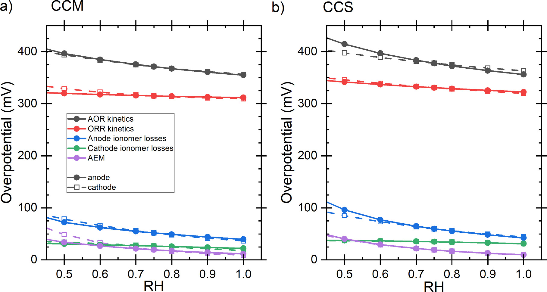
Figure 12. The effect of the anode (solid symbols and lines) and cathode (open symbols and dashed lines) side RH on the voltage losses at 50 mA cm−2 current density with (a) CCM and (b) CCS.
Download figure:
Standard image High-resolution imageAt least a part of the increased sensitivity to the cathode side RH is that the cathode CL of the CCM is thinner than the other simulated ionomer-containing layers, making it the least resistive to water transport through it. The water flux at both cathodes is in from the O2 flow, but with CCS the magnitude is higher, so from this it could be expected that CCS would be more strongly coupled to cathode RH through the cathode-side outflux boundary condition (Eq. 51). As the opposite is true for the sensitivity of the power density to the cathode RH, and because the effects on the anode side losses were an important difference, the CL layer thickness and water transport resistance appears a more likely explanation. The reduced AOR losses are probably due to the increased ionomer conductivity increasing the driving kinetic overpotential farther from the AEM. This increases the AOR rate there, meaning that, for the same total current density, the AOR rate near the AEM could be lower, reducing the kinetic overpotential. Due to the functional form of the AOR kinetics, at the ca. 400 mV overpotentials where the current density is near the saturation to A (see Fig. 1, a relatively small reduction in the local reaction rate could reduce the overpotential more than the corresponding increase in the AOR rate elsewhere requires the overpotential to increase.
The spatial distribution of water activity (RH) for the baseline scenario at 93 mA cm−2 current density is illustrated in Fig. 13. Qualitatively, the CCM profile is in agreement with the neutron radiography results of Omasta et al. 72 and the simulated water content profile of Gerhardt et al. 52 (in their SI) for AEM HFC. Despite the different FC types (HFC vs DAFC), a direct comparison is valid because the most important physics and boundary conditions of water transport are the same (humidified gaseous feeds, AEM, the same numbers of electrons per water molecule in both reactions). The electro-osmotic drag, generation of water by the AOR, and consumption by the ORR bias the peak RH towards the anode, and back diffusion to the cathode is responsible for the RH remaining slightly higher than the inflow RH near the AEM. While in our case the peak is in the CL side of the anode CL-AEM interface (Omasta et al. had it in the AEM), this is likely influenced by our higher catalyst loadings, thicker CLs, and thinner AEM. Because the water outflow rate depends directly on the difference to the inflow RH, in this case 0.75 (see Eq. 51), the greatest water outflux is at the CCS anode and at the cathodes the flux is in from the gas channel rather than out of the electrodes. The maximum RH in the CCS is higher than in CCM, which could lead to earlier flooding in the cell, and especially CCS cathode might suffer from drying at low cathode inflow RHs. The cathode water influx is larger with CCS so the magnitude of the flux likely does not explain the higher sensitivity of CCM to the cathode RH, which might be due to the CCS electrode being more restrictive to gas transport than the substrate without the ionomer in the case of CCM.

Figure 13. The spatial profile of the RH (or water activity in the ionomer) in the DAFC in the baseline scenario at 93 mA cm−2 current density (0.25 V with CCM, 0.19 V with CCS). The x-axis is scaled so that 0 mm, indicated by the vertical line, is at the middle of the AEM (the light blue area), and negative values are in the anode and positive in the cathode side of the DAFC. The solid black line corresponds to the CCM, the red dashed line to the CCS, and the horizontal dashed line to the 0.75 inflow RH. The inset shows the profiles near the AEM.
Download figure:
Standard image High-resolution imageAs a difference to experimental results that indicate CCS to have lower mass transport resistance than CCM, e.g., 41,73 in our case the CCS has no clear separate CL, and catalyst and ionomer fill the entire PTL substrate thickness, and this difference would affect mass transport through the electrode. Our catalyst loading is also significantly higher than in HFC literature, about 10-fold difference (or even more), which could affect the comparison. It is not clear how a reduced CL thickness and partially filled porous substrate would affect water transport, but we consider this analysis to be outside the scope of the study. The simulation model could also overestimate the diffusion coefficients inside the porous layers, which could affect the overall mass transport in the CCM and CCS simulations differently due to different layer thicknesses and porosities.
The gas flow rate has an important role in humidity management by controlling the removal rate of the produced water. Compared to PEM HFCs with dry cathode stream, the humidified cathode stream and electro-osmotic drag moving water to the anode reduces the capacity of the cathode stream to accomplish this, similarly to AEM HFCs. In fact, although the simulated AEM was quite thin, in principle helping back diffusion towards the cathode, varying the cathode gas flow rate had practically no effect on the DAFC output power or the RHs at the electrode - gas channel interfaces. The power density as a function of gas flow at 0.25 V and at 50 mA cm−2 current density is shown in Fig. 14. Except for the sharp decrease below ca. 0.5 ml min−1 cm−2, the cathode side flow has only a very small effect on the DAFC output power and both the anode and cathode RHs (Fig. S9). With the anode flow, there is a maximum at about 3 ml min−1 cm−2 due to reduced water removal, i.e. increased RH and ionomer conductivity (Fig. S9), but not yet too diminished ammonia supply. In practice, the larger effect of the changed downstream composition (Fig. 7) would mean that reducing the gas flow rate almost certainly would reduce the DAFC power, instead of increasing it.
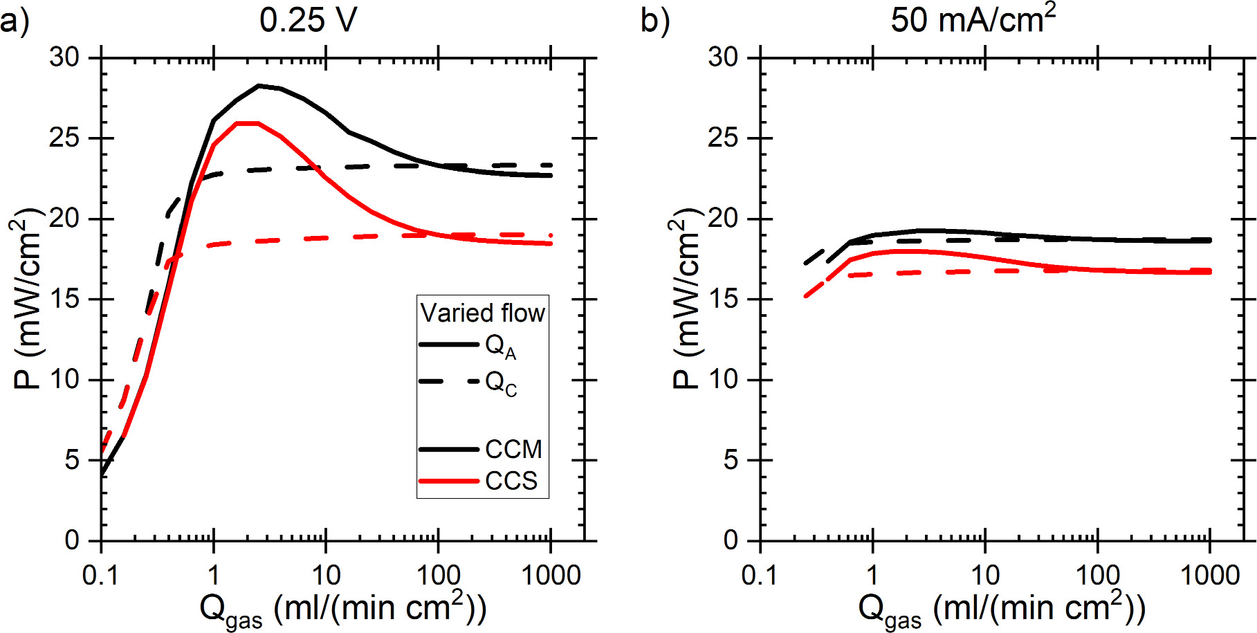
Figure 14. The power at (a) 0.25 V voltage and (b) 50 mA cm−2 as a function of the anode (solid lines) or cathode (dashed lines) gas flow rate with the other flow fixed to 100 ml min−1 cm−2. The black lines correspond to the CCM and red to the CCS.
Download figure:
Standard image High-resolution imageThe peak in power at about 3 ml min−1 cm−2 is because our model is a point model, when considering the geometric area of the electrodes and thus does not account for any nonuniformities, due to e.g. gas composition change along the flow channel, over the electrode area. Additionally, the downstream effects could make the DAFC more sensitive to the gas composition or flow rate than our simulations suggest. That said, optimization for better humidity retention in the cell could improve the DAFC performance, provided that the transport of the other species would not be severely impeded.
The gas flow rate can be interpreted as either the gas volume flow per electrode area or the gas velocity (as mentioned earlier, ml min−1 cm−2 is in fact equal to cm min−1). Because we do not consider nonuniformities over electrode area or channel length, the simulated effects probably match small electrode areas the best. With increasing electrode area, the gas velocity typically increases faster than the volume flow per electrode area: The average velocity is the function of the flow field channel layout and the total gas flow rate. Because the gas channel cross section typically does not increase as fast as the electrode area, increasing the electrode area while maintaining a constant gas flow per electrode area would increase the gas velocity in the channels. Therefore, the effects primarily related to the reactant supply rate (flow rate per area) and gas velocity may impact a DAFC differently with different electrode areas.
Gas composition
Figure 15 shows the effect of the fraction of ammonia and oxygen of the dry anode and cathode inflows, respectively (fk in Eq. 52). In the baseline scenario the fraction of both is 0.5, or 50%. Similarly to most scenarios with the other parameters, in general the CCM produces few mW cm−2 higher power at all values. The pattern of the Nernst voltage (Fig. S12) at the same cell voltage shows the same pattern with the highest power matching the highest thermodynamic voltage. The reaction kinetics are also affected, with increasing ammonia fraction decreasing the AOR and oxygen fraction ORR losses (Fig. S13), except that AOR losses increase slightly when ammonia fraction increases to over 0.9, and the further increased power is probably due to increased thermodynamic voltage. In both cases the ammonia concentration is more important than the oxygen concentration, higher power densities can be achieved or maintained with low oxygen concentration than with low ammonia concentration. The reaction stoichiometry certainly affects this: three electrons per NH3 molecule and four per O2, meaning that at any current density NH3 is consumed faster than O2, and the AOR Nernst potential is more sensitive to the NH3 partial pressure than the ORR potential to the O2 partial pressure (∼20 mV/decade vs ∼15 mV/decade). The difference may be smaller than in HFCs (2 electrons per H2, thus ∼30 mV/decade), but the NH3 supply rate likely still needs to be higher than the O2 supply rate to avoid gas composition problems along the flow channels.

Figure 15. The simulated effect of the molar fraction of ammonia and oxygen in the dry gas inflows in the case of (a) CCM and (b) CCS.
Download figure:
Standard image High-resolution imageThe AOR and ORR concentration overpotentials (Eqs. 12 and 13) for the CCM are shown in Fig. 16. In the case of the AOR, negative concentration polarization corresponds to increased DAFC voltage, whereas in the case of the ORR more positive potentials increase the DAFC voltage. The differences compared to the CCS were negligible. While the contours are neither perfectly horizontal nor vertical, they are very close to it, demonstrating that other factors did not meaningfully contribute to the equilibrium potentials. Comparing the AOR and ORR potentials to each other, the difference between the maximum and minimum for the ORR was about 30 mV compared to about 65 mV of the AOR, quantifying the higher sensitivity to the ammonia concentration. This result was of course affected by our choice of using N2 as the non-reactant component of the dry gas mixture. Alternatively, N2 being a very common inert gas means that its contribution to the AOR Nernst potential magnifies the sensitivity of DAFCs to the anode gas composition, when compared to other FC types. Nevertheless, changes to the ammonia pressure corresponded to about 45 mV and N2 pressure to about 20 mV of the total 65 mV change (Fig. S14), meaning that NH3 alone affected the thermodynamic voltage about 50% more than O2. In practice, it may therefore be necessary to operate a DAFC with higher anode side flow rate or/and pressure than the cathode side to minimize voltage losses especially due to composition gradients along the flow channel.
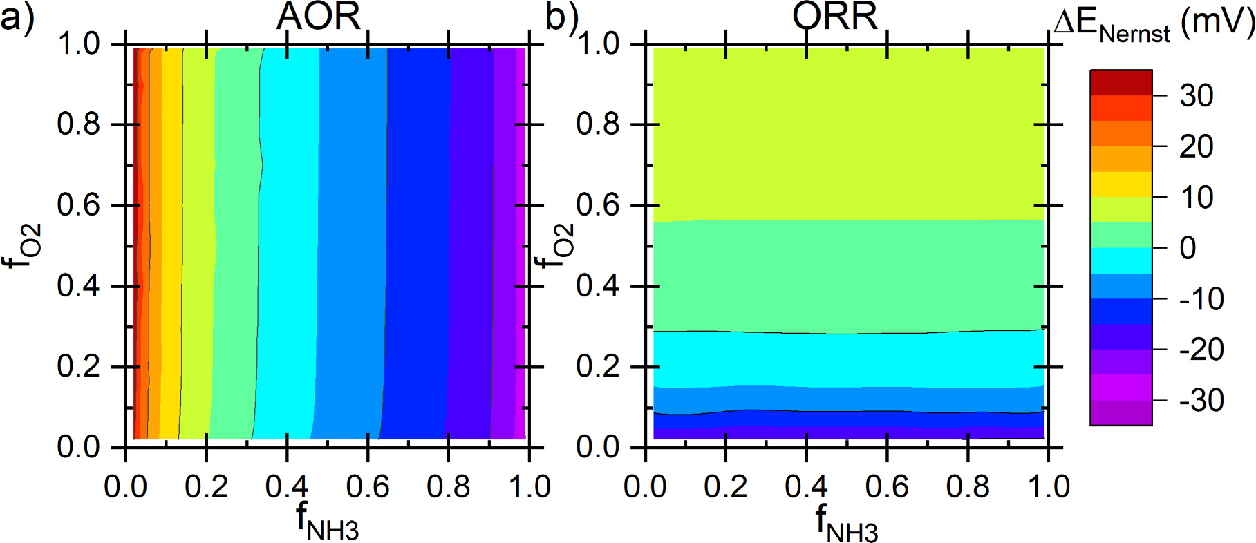
Figure 16. The AOR (a) and ORR (b) concentration polarizations at 250 mV for the CCM. Negative values correspond to the equilibrium shifting to more negative potentials, meaning that negative AOR and positive ORR potentials increase the DAFC voltage. In both figures, 0 mV corresponds to 1 bar partial pressures and RH = 1 (or to any combination of pressures and RH that yields 1 inside the logarithm in Eqs. 12 and 13).
Download figure:
Standard image High-resolution imageWhile the performance in Fig. 15 correlates positively with the thermodynamic voltage of the cell, in other cases this connection does not necessarily exist. For example, in the case of the catalyst loading, the highest powers corresponded to the lowest thermodynamic voltages (Figs. 10 and S15), and in the case of CCM to the highest peak RH inside the cell (Fig. S10), the match between the peak RH and Nernst voltage being especially striking. Therefore, the best performance corresponded to the best capability to extract power from the available reactants, not to the best gas transport. In the case of the catalyst loading and CCM specifically, the general trend of the thermodynamic voltage appears to be dictated by the anode and the peak RH, as increased cathode RH would increase the voltage. Increased anode RH would, of course, reduce ion transport losses and maybe also reduce the average kinetic overpotential. Similarly to Fig. 16, the anode RH is more important to the Nernst voltage than the cathode RH due to reaction stoichiometries, AOR (reaction (2)) producing a water molecule for each electrode, whereas ORR (reaction (3)) requires 2 electrons for each consumed water molecule, further amplifying the importance of the anode gas composition on the DAFC performance compared to the cathode.
Pressure
Compared to the temperature and the RH, the effect of increased pressure was small. However, when considering the ultimate, achievable performance of a DAFC, the pressure can be multiplied, whereas the maximum RH and temperature increases are limited closer to the 20% of our sensitivity analysis. (The temperature limit is due to material constraints, and solid oxide fuel cells could be operated at much higher temperatures. 11 ) As shown in Table II, the anode gauge pressure had a larger impact on the power density than the cathode pressure and increasing it to 5 bar (with constant mass flow) increased the power to 29.1 mW cm−2 with CCM and to 23.7 mW cm−2 with CCS. Pressurizing both electrodes to 5 bar increased the power densities to 32.8 mW cm−2 and 26.1 mW cm−2 with CCM and CCS, respectively. Compared to the 20% changes to the other parameters in Fig. 7, increasing the anode pressure has roughly the same impact as increasing the RH of one electrode, and pressurizing both electrodes to 5 bar has roughly the same impact as increasing the cell temperature. The effect of the gauge pressures is plotted in Fig. 17. Therefore, although minor changes to pressure had only a small impact on the cell performance, if the cell can be properly pressurized, the performance gains are comparable to the effects of increased temperature and RH. The main cause of the enhanced performance were the reduced kinetic overpotentials, especially of AOR with increased anode pressure, as shown in Fig. S16. The other voltage losses were almost not affected at all.
Table II. The simulated effect of increasing gauge pressure from 1 bar to 5 bar on the DAFC power at 0.25 V voltage and 75 mA cm−2 current density, while maintaining a constant mass flow to the cell, corresponding to 100 ml min−1 cm−2 at 1 bar gauge pressure.
| Power density at 0.25 V/75 mA cm−2 (mW cm−2) | ||
|---|---|---|
| Gauge pressures, A/C (bar) | CCM | CCS |
| 1/1, baseline | 23.3/22.7 | 19.0/19.0 |
| 1/5 | 25.1/24.3 | 20.4/20.5 |
| 5/1 | 29.1/26.3 | 23.7/23.0 |
| 5/5 | 32.8/28.3 | 26.1/25.0 |

Figure 17. The effect of the gauge pressure (solid lines - anode, dashed lines - cathode, short dashes - both) on the DAFC power at 0.25 V with CCM (black lines) and with CCS (red lines). The mass flow corresponds to 100 ml min−1 cm−2 under 1 bar gauge pressure and we assume the ideal gas law.
Download figure:
Standard image High-resolution imageCombined effect of all parameters
The result of summing together all power increases or decreases in Fig. 7 is shown in Table III below. Here, we have considered the effect of increasing e.g., the RH and pressure of both the anode and cathode at the same time, but not the separate effects of changing a parameter at the anode without changing it at the cathode, or vice versa. For comparison, we also simulated the effect of simultaneously increasing or decreasing all parameter values by 20%. Overall, the magnitude of the sums of the separate increases and decreases are closer to each other than to the simultaneous increases and decreases. The absolute changes with the CCS are smaller than with the CCM, which probably only reflects the lower baseline power, as the relative changes are a little larger than with the CCM.
Table III. The absolute and relative power density changes with separate and simultaneous changes to the DAFC and operating condition parameters.
 P(mW cm−2)/ P(mW cm−2)/ P/P0 (%) P/P0 (%) | ||
|---|---|---|
| Change to the parameters | CCM | CCS |
| −20%, separate | −24.1/−103 | −21.4/−112 |
| −20%, simultaneous | −16.1/−69 | −13.7/−72 |
| +20%, separate | +27.1/+116 | +23.8/+125 |
| +20%, simultaneous | +39.1/+168 | +36.1/+190 |
When the parameter values are decreased simultaneously, the effect is less than the sum of separate decreases, whereas the simultaneous increase yields higher power than the sum of the separate increases. This shows the nonlinearity of the response to the simultaneous increase or decrease of all parameters. Separate changes of a single parameter at a time cause overall smaller, and thus presumably more linear response. In the case of reduced parameter values, the simultaneous reduction has the effective limit that the resulting power almost certainly must remain positive, which does not apply to the sum of separate changes. Considering the power, except for the interval 1.05–1.25 in Fig. 18, the curves are clearly nonlinear, with larger parameter increase yielding larger power increase up to 25% increase, after which the increased ionomer volume fraction (0.975) constricts the gas diffusion.
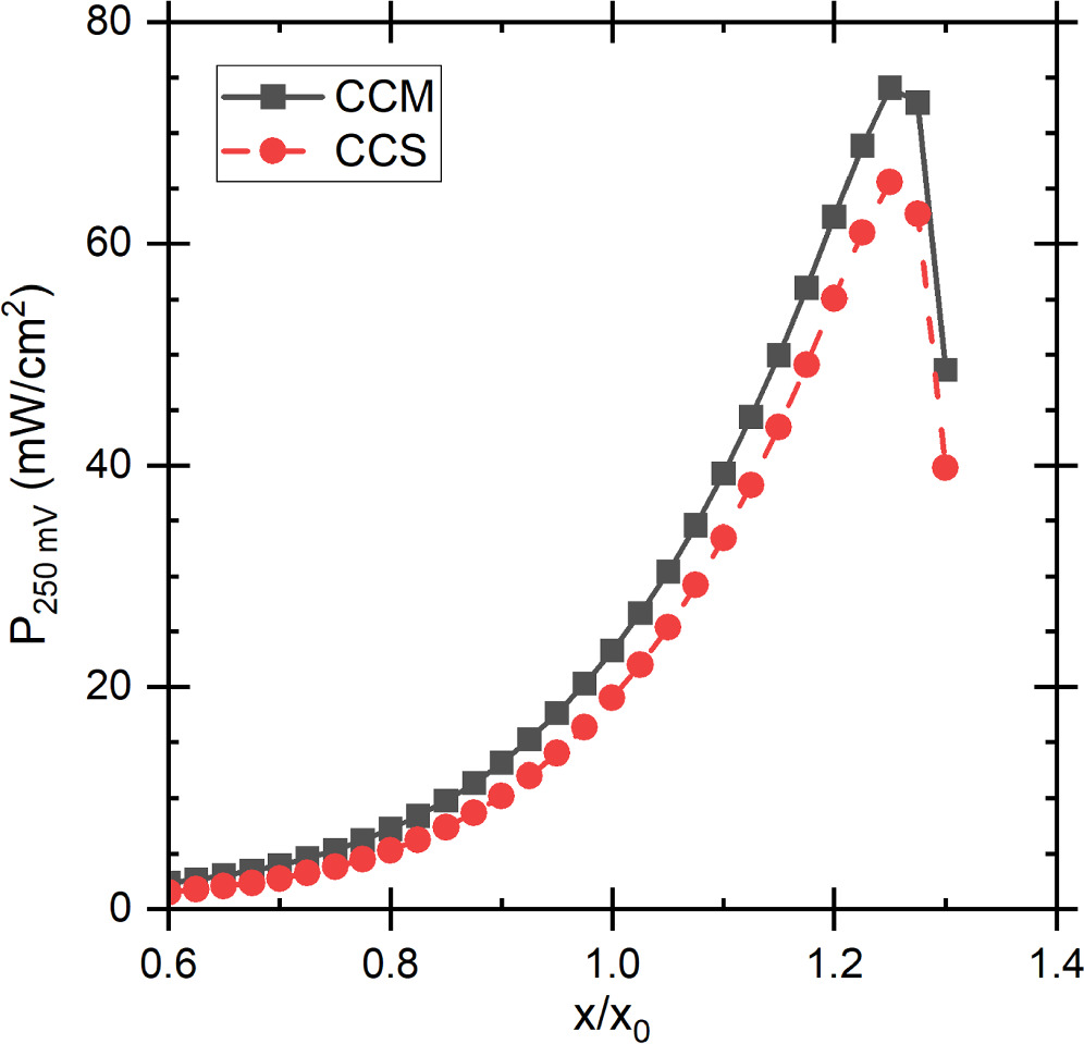
Figure 18. The simulated DAFC power at 250 mV as a function of the magnitude of the simultaneous parameter increase (x/x0>1) or decrease (x/x0<1).
Download figure:
Standard image High-resolution imageThe voltage loss breakdown at 50 mA cm−2 is shown in Fig. 19. Overall, the differences between the two electrode structures are not immediately obvious, but there are few:
- higher cathode ionic transport losses with the CCS
- kinetic overpotentials and anode ionic transport losses decrease faster with increasing parameter values with the CCS.
The AEM losses are very similar, so there are likely no significant differences in water uptake and AEM conductivity. At parameter value 1.3, the ionomer volume fraction is high enough to affect gas transport, but the 50 mA cm−2 current density in Fig. 19 is too low for the gas transport to constrict the DAFC performance yet. Considering the operation at 0.25 V voltage, on the other hand, clearly shows a sharp reduction in kinetic overpotential with an increase in anode or cathode ionic transport losses, depending on the electrode type (see supporting information). From 1.25 to 1.30, the concentration polarizations increase sharply and the thermodynamic voltage reduces.
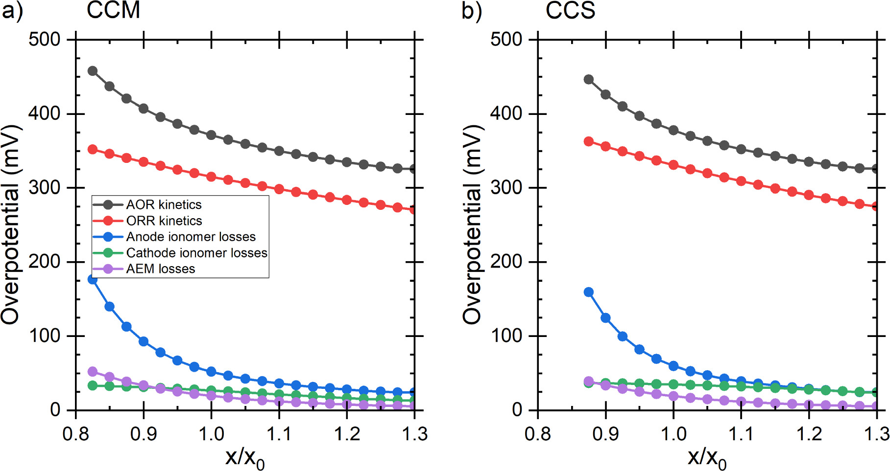
Figure 19. The voltage loss breakdown at 50 mA cm−2 for the simultaneous parameter value change for (a) CCM and (b) CCS. The missing lower range is due to those parameter combinations being limited to lower current densities.
Download figure:
Standard image High-resolution image
Discussion
We developed a 1D cross-section model of gas-fed DAFC that we verified against the experimental data and a model provided by Zhao et al. 23 While the temperature dependency of our model is clearly different from both their measurements and simulations due to the AEM and ionomer parametrization, at current densities below the maximum power point (or at over ca. 0.25 V voltage) the models were within 5% of each other in our comparisons. The error compared to experimental data at higher current densities is probably caused by the AOR kinetics parametrization slightly overestimating voltage losses. Compared to their model, we can study the effects of concentrations, or partial pressures, and mass transport phenomena everywhere in the cell, not only in the anode CL. The coupling of e.g. ionic conductivity to water uptake allows us to simulate the effects of the operating conditions both on the cell as a whole and on the spatial distributions in the cell.
Our simulations showed that the cell temperature and RH were the parameters that most affected the DAFC power, even with the reduced temperature sensitivity of ionic conductivity due to the AEM and ionomer parametrization (discussed in "Validation by literature comparison"). This result is generally similar to literature on AEM HFCs. 35,68 The AOR kinetics were the largest voltage loss component and the one that typically varied the most with changes to the operating conditions. While the ORR kinetics was the second largest voltage loss component, quite often the anode ionic transport losses were more sensitive to the operating conditions, which is most likely due to their coupling to the AOR kinetics. The major difference between the electrode structures was the higher sensitivity to the catalyst loading with the CCS, or the lack of effect due to ionic transport losses with the CCM. Another difference is that the optimal ionomer loading of a CCS could be lower than that of a CCM to avoid constricting gas transport due to the difference in the thickness of the ionomer-containing layers. In principle, the optimal ionomer loading (and more generally, electrode porosity and other properties) could also depend on the expected maximum current density, as higher reaction rates would require higher mass transport rates. Due to the higher catalyst loadings and lower current densities compared to HFCs, the optimal ionomer loading of a DAFC could be therefore somewhat different than in a HFC.
Although the simulations suggest that reduced anode gas flow rate could increase the power density through increased RH and ionic conductivity, this most likely will not happen in a real DAFC. (The cathode flow rate had practically no effect, except for constricting the cell operation at too low O2 supply rates.) Our model is effectively a point model when considering the geometric electrode area and, in reality, the higher sensitivity to the downstream composition changes should reduce the power when the gas flow rate is decreased. This could also make the DAFC performance more sensitive to the gas composition and flow rate changes than our simulations indicate. More accurate studies about the flow rate effects would need a model that can properly describe the downstream composition changes, including the RH, because flooding at high RHs could significantly reduce the average power density.
The reaction stoichiometries make the DAFC more sensitive to the anode than to the cathode. This was quantified by the anode concentration polarization changes being about twice as high as the cathode concentration polarization changes, and ammonia causing about 50% higher losses than oxygen, when the gas flow compositions were varied. The remaining part of the anode component was due to the change in the nitrogen partial pressure because N2 is produced by the AOR, and we used it as the non-reactant component of the gas mixtures. Similarly to the AEM HFCs, and contrary to PEM HFCs, water management is complex. Water generation by the AOR and electro-osmotic drag bias the maximum RH towards the anode and water removal from the cathode is very limited, unless the cathode RH is significantly reduced. Although a very minor effect of the RH, also the anode RH affects the thermodynamic voltage more than the cathode RH, which is magnified by the peak RH being located in the anode. Because it is likely necessary to supply more gas to the anode than to the cathode, DAFC being more sensitive to NH3 than to O2, using dry anode gas could be useful to limit the maximum RH, but this would also severely reduce the power output. Despite receiving almost none of the produced water, the cathode RH impacts the DAFC power almost as much as the anode RH (or even more with the CCM), so the best water management strategy could to some extent be case by case, and a more specific study would be needed for more precise conclusions. As with the effects of the gas flow rate, this is of course subject also to the downstream gas composition changes and their effect on water removal in a real DAFC.
As the effect of the catalyst loadings on the kinetic overpotentials showed, water transport couples the electrodes together and, technically, they cannot be optimized fully separately. Because the dependence of the AOR losses on the cathode catalyst loading was noticeable only at high catalyst loadings and relatively small in magnitude, in practice this can be safely neglected in almost all cases. Nevertheless, it serves as a reminder that changes to any part of the cell affect all other components as well, to some degree, through the transport processes in the cell.
While there might not be any simple ways to increase the DAFC power, mapping the operating conditions and the most important cell parameters helps to prioritize those with the most impact over the less effective ones. Similarly, the relative sensitivity of the voltage losses, basically the anode being more sensitive than the cathode, helps to direct the research and development to the parts of the cell that most affect its performance. Except for the clear priority of the AOR catalysts and increased sensitivity to the anode ion transport, the most important factors seem similar to AEM HFCs. 35,68 Quite surprisingly, in some cases the catalyst loading could have only little effect on the power. Therefore, the electrode structure is also an important parameter when considering how to optimize the DAFC performance. Sometimes changes that intuitively should increase the cell power might not accomplish that, and device modeling can help to understand the physics and chemistry involved.
Conclusions
We have developed a one-dimensional model of the DAFC cross-section to study the operation, specifically interactions between reaction kinetics and different transport phenomena. The model was validated against another that had also been calibrated with experimental data. We used the model to perform a sensitivity analysis for several parameters related to the cell operating conditions (e.g., temperature, relative humidity) and properties (e.g., catalyst loading). Clear differences in the effects of parameters in our study already indicate, for instance, temperature and relative humidity (RH; via reaction kinetics and ion transport losses) having the highest impacts on the DAFC power density. Also, electrode kinetics being coupled to each other via water transport are not fully independent of each other, although the practical effect may be small. CCS is more sensitive to catalyst loading and less sensitive to cathode relative humidity than CCM. A more comprehensive model would be needed to fully quantify, for instance, the effects of the gas flow rate and downstream composition changes, and thus optimal humidity management strategies.
Acknowledgments
This research was done under the TELEGRAM project. This project has received funding from the European Union's Horizon 2020 Research and Innovation programme under grant agreement No 101006941. The project started on the 1st of November 2020 with a duration of 42 months.
Supplementary data (1.7 MB PDF)