

Abstract
As the most routine work practice in an aluminum reduction cell, anode change introduces substantial perturbations that adversely affect the mass and heat balance of the cell which may lead to loss of process efficiency and increased energy consumption. The literature lacks a dynamic mathematical model that describes the interactions among cell variables (e.g., electrolyte temperature and flow, anode current distribution, and cell heat loss) during and following this operation, which could otherwise be used to understand the process in greater depth and to develop changes that improve process operations and control. This paper presents a spatially-discretised dynamic model for anode replacement that integrates mass balance, thermal balance and cell voltage to describe and predict local cell variables. It was experimentally validated with an industrial cell undergoing an anode change procedure. This generic model can be applied to different cell design or process conditions by using appropriate parameters (e.g., heat transfer coefficients, conductivities, and flow patterns). The model can be used to improve existing process operations or control strategies for higher process efficiency, lower energy consumption, and lower emissions.
Export citation and abstract BibTeX RIS
| List of Symbols | |
| A | Cross-sectional surface area |
| accum | Rate of metal accumulation |

| Effective anode surface area |
| BM | Beam movement control action |
| c | Heat capacity of subsystem |
| C | Mass composition of electrolyte |
| consum | Rate of carbon consumption |
| D | Anode-to-cathode distance (ACD) |
| EE | Cell reversible potential |
| expand | Rate of thermal expansion of anode and assembly |
| F | Faraday's constant |
| h | Heat transfer coefficient (HTC) |
| Han | Height of anodes |
| ΔHfus | Heat of fusion of cryolite |
| I | Line current |
| Ian | Anode current |
| k | Thermal conductivity |
| kdiss | Alumina dissolution rate |
| L | Length through which heat conducts |
| m | Mass |
| M | Molecular weight |
| mfed | Mass of alumina fed |

| Rate of aluminum production |

| Rate of alumina transferred by electrolyte flow |
| Q | Rate of heat transfer between two subsystems |
| r | Proportion of quick dissolving alumina in feed |
| R | Thermal resistivity |
| t | Time |
| T | Temperature |
| Tliq | Liquidus temperature |
| v | Electrolyte flow velocity |
| V | Volume of subsystem |
| Vcell | Cell voltage |
| Vext | External voltage drop |
| z | Number of charges transferred |
| Greek | |
| η | Current efficiency |
| ηover | Cell overpotentials |
| ρ | Density of material |

| Electrical resistivity of anodes |
| Subscripts | |
| an | Anode |
| amb | Ambient potroom air |
| elect | Electrolyte |
| bub | Bubble |
| ca | Cathode |
| fr | Freeze |
| hood | Hooded environment in cell |
| s | Surface |
| ∞ | Far away from surface |
| in | Received by subsystem |
| out | Leaving subsystem |
| gen | Generated in subsystem |
Since 1889, the Hall-Héroult process has remained as the only method to commercially produce aluminum via the electrolysis of an alumina-cryolite melt, 1,2 with its electrochemical extraction being dominated by the following overall chemical reactions where carbon anodes are continuously consumed during the process: 3


According to the International Aluminium Institute, 4 the total global primary aluminum production has reached 65.3 million tonnes in 2020. Among other limitless applications, the transport sector continues to drive this demand to improve fuel efficiency and reduce emissions by having lighter vehicles. 3 The demand is predicted to double or triple by the year 2050. 5 Aluminium production has been steadily increased to meet this rising demand, but the scalability of the industry is mainly challenged by the inefficiencies in the energy-intensive process. Virtually all present operating technologies require electrical energy of between 13 and 16 kWh/kg Al. 3 However, only between 6.5 and 6.65 kWh/kg is used for the process; the remainder being wasted through cell heat loss, Faradaic and other inefficiencies arising from cell design, anode carbon reactivity, and operating work practices. While the scientific knowledge established from experience enables optimisation of process conditions for any given cell design and operating line current, all cells are subject to a substantial perturbation of the thermal balance of the cell by the regular practice of anode replacement. 6 Typical anode sizes used in modern technology remove a minimum of 50 kWh of stored energy from a localised zone and introduces a demand for more than 160 kWh to reinstate optimum cell conditions at its required operating temperature of near 960 °C. This substantial perturbation occurs every 30 to 36 h. 7 With the growing need to move to an electrical energy source society, there is a greater need for both increased productivity and high energy efficiencies in aluminum smelting since it is such a high electrical energy consumer. While complex CFD models have been developed to improve process understanding and design (e.g., 8–12 ), and model-based process monitoring and control approaches have been developed to improve operation performance based on target conditions (e.g., 13–18 ), more advanced dynamic models that can enable simultaneous optimisation of both the process and the energy consumption are needed, especially during and following the anode change operation.
As anodes at their end of service life are replaced with new anodes, each newly inserted cold anode preferentially solidify cryolite from the solvent electrolyte mixture, forming a current-blocking layer of freeze that soon extends down to the molten aluminum (cathode), impeding the flow of the electric current through the new anodes (see Fig. 1). As cryolite freezes selectively, this alters the chemical composition and therefore the liquidus temperature, as well as affecting the electrolyte temperature and changing the driving force for heat transfer. The resulting change in localised conditions simultaneously and adversely affect the thickness of a similar cryolite-based freeze lining of the cell wall known as the ledge, which is required to protect the materials of construction from the corrosive environment and minimize cell heat loss. As a cell typically has at least 16 anodes or anode pairs connected in parallel, the regulated current is redistributed to the other anodes in the cell, which leads to further non-uniformity in material consumption and heat generation. Over the years, numerous adverse effects can be directly attributed to inappropriate operating response to anode changes, including improper feed dissolution, sludge formation, and anode spike formation, 7,19 leading to short-circuiting and all contributing to loss of process efficiency and an increase in energy consumption.

Figure 1. Anode freeze (frozen electrolyte underneath an anode) impeding the flow of current through that anode.
Download figure:
Standard image High-resolution imageWhile numerous dynamic reduction cell models exist (e.g., 20–22 ), the operating conditions and energy and productivity priorities during an anode change event are not well served by the previous approaches. In this manuscript, based on our previous work 23 that investigated how various mechanisms affect the pickup of anode current after anode replacement, we present a model with integrated mass and energy balances to describe the freeze dissolution and heat transfer from the first principle with less reliance on empirical relations. This model can improve existing anode replacement operations or control algorithms by providing insights into this routine operation, for example by deciding any necessary adjustments to the height at which anodes are clamped in order to achieve a desirable rate of anode current pickup based on predictions of its future trajectory. By limiting the disturbance to the process and thereby increasing the energy efficiency, this model plays an important role in helping us use energy more thoughtfully and responsibly as the industry scales up the production.
Model Development
Coupled model features
A spatially-discretised mass balance model, thermal balance model, and cell voltage model must be integrated together to capture the strong coupling effects between process variables, which are mostly left out of previous spatial models. Some important considerations include:
- Alumina consumed during the reaction is replenished by feeders in the cell. Each dump of alumina feed absorbs energy from the electrolyte for preheating and dissolution.
- The freeze (anode freeze and side ledge) can be assumed to be pure cryolite. Therefore, as they form from or dissolve back into the electrolyte, the composition of electrolyte changes.
- Due to the formation or dissolution of freeze, the height of electrolyte changes, which changes the area for heat transfer and therefore affects the thermal balance. The change in electrolyte height depends on the difference between cryolite and electrolyte densities, as newly-formed freeze displaces the electrolyte and vice versa.
- Change in electrolyte composition affects the liquidus temperature, which helps drive the freeze dynamics. The side ledge insulates the cell from further heat loss, so changes in ledge thickness further affects the thermal balances.
- Presence of freeze underneath a new anode acts as additional path resistance which impedes current flow, which has to be redistributed to the other anodes. As the freeze dissolves, more anode area will be exposed and path resistance will decrease and restore to previous value.
- The dissolution of freeze underneath a new anode reduces the local electrolyte temperature, and hence the heat transfer out the sidewall in that zone. This causes a growth in the local side ledge thickness.
- The redistribution of anode current causes the local alumina and carbon anode to be consumed at different rates as per Faraday's law of electrolysis. This changes the mass composition as well as the anode-to-cathode distance (ACD).
- Changes in electrolyte composition, anode height, or ACD due to material consumption changes the total path impedance, which causes anode current to redistribute and cell voltage to change. Both of these consequently affects the heat generation.
- The temperature of the electrolyte also affects cell voltage, which affect heat generation, freeze dissolution, and ultimately electrolyte composition.
Spatially-discretised thermal model
The measurement of individual anode currents in a cell is unconventional, but has shown great benefits for cell monitoring and control. 24–34 As the heat generation in a cell is primarily ohmic, the anode current distribution readily represents the spatial distribution of energy in a cell. Therefore, similar to the work first presented by Cheung, 26 regions in the cell are discretised according to anode locations as shown in Fig. 2 in order to capture the dynamics of local thermal variables during anode change.
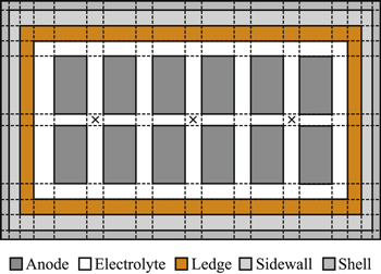
Figure 2. Illustration of spatial discretisation of the thermal model using a simplified cell with 12 anodes and 3 alumina feeders (×).
Download figure:
Standard image High-resolution imageThe vertical layers of electrolyte and aluminum metal are not further discretised in this approach as the magnitude of anode current already reflects the total interelectrode path impedance due to electrolyte resistance, bubble layer resistance, as well as overpotentials in the electrochemical reaction. 21,26 Therefore, local heat generation can be easily calculated from the cell voltage and anode current. By eliminating empirical Eq.s. and constants for electrical resistances from the thermal model, this increases the versatility of the thermal model as actual measurements of cell voltage and anode currents can also be used as model inputs, while for simulation studies, cell voltage and anode current distribution can still be calculated as shown in a later section.
The governing thermal equations, as well as the domains they are applicable in, are summarised in Table I, and more details are provided in the following sections. The key model parameters used in this paper are provided in Tables II and III, and they are specific to the cell technology, cell design and process conditions in this work. As the temperature of an anode changes drastically after replacement, its thermal conductivity is provided as an equation in Table II.
Table I. Common governing thermal Eq.s. in the model.
| Parameter | Domain | Governing equation | |
|---|---|---|---|
| Heat transfer | |||
| Conduction | Electrolyte, metal, ledge, sidewall, shell, ledge–sidewall, sidewall–shell, anode–crust, electrolyte–crust, freeze–anode, anode–assembly, bottom insulation–shell. |

| [3] |
| Convection | Anode-electrolyte, electrolyte–ledge, metal–ledge, electrolyte–freeze, metal–freeze, shell–ambient, crust–hood, assembly–hood, rod–ambient. | Q = hA(Ts − T∞) | [4] |
| Advection | Electrolyte flow | Q = ρ Avc(T1 − T2) | [5] |
| Thermal resistance | |||
| Heat flow | All subsystems. |

| [6] |
| Conduction | Same as conduction above. |

| [7] |
| Convection | Same as convection above. |

| [8] |
| Derivative of state | |||
| Temperature | All subsystems. |
| [9] |
| Mass of frozen electrolyte | Ledge and anode freeze. |

| [10] |
| Mass of electrolyte | Electrolyte. |

| [11] |
| Other | |||
| Faraday's law of electrolysis | Anode consumption, alumina consumption, metal production. |

| [12] |
Table II. Thermal conductivities of materials in the model.
| Material | K | References |
|---|---|---|
| (W/(m K)) | ||
| Anode 3 × 10⁻⁶ T2 − 0.001T + 4.9624 | Industry | |
| Electrolyte | 1000 | 26 |
| Metal | 1000 | 26 |
| Cryolite (Freeze/ledge) | 1–1.5 | Industry |
| Graphitised block (sidewall) | 58-77 | Industry |
| SiC block (sidewall) | 22–31 | Industry |
| Steel shell (side) | 42–47 | Industry |
| Cast steel (yoke) | 38.6 | Industry |
| Rod | 210 | Industry |
| Crust | 2.6 | Industry |
| Collector bar | 30 | Industry |
| Firebricks | 1.50 | 26 |
| High-density vermiculite | 0.30 | Industry |
| Low-density vermiculite | 0.14 | 26 |
| Steel shell (bottom) | 31 | 26 |
Table III. Heat transfer coefficients (HTC) in the model.
| Material | h | References |
|---|---|---|
| (W/(m2 K)) | ||
| Electrolyte—anode | 1100 | 26 |
| Electrolyte—ledge | 600 | Industry |
| Metal—ledge | 1250 | Industry |
| Side shell—ambient | 22 | Industry |
| Bottom shell—ambient | 20–30 | Industry |
| Rod—ambient | 40 | Assumed |
| Rod/yoke—hooded ambient | 40 | Assumed |
| Crust—hooded ambient | 20-40 | Industry |
Heat generation
The local electrical power input into the cell can be calculated from the anode current, Ian , and cell voltage, Vcell . However, the energy lost due to voltage drop across bus bar external to the cell, Vext , and the electrochemical energy used for process reactions do not contribute toward cell heating. The latter amounts to about 6.60 kWh/kg Al (see Table IV), based on a net and gross anode carbon consumption that of a modern technology of 0.40 kg/kg Al and 0.50 kg/kg Al respectively. 35 As this model computes the local heat requirement for the feed and anode only when they are introduced into the electrolyte, the energy that is not used for heat generation reduces to 5.294 kWh/kg Al. Thus, the local heat generation rate at each anode, Qgen , is given as

where  is the rate of metal production as given by Faraday's law of electrolysis (Eq. 12). In the equation, η is the current efficiency, M is the atomic mass of aluminum (26.98u), F is the Faraday's constant (96,485 C/mol), and z is the number of charges transferred (3). A portion of this heat energy is generated in the anode, with a rate of Qgen,an
, given by
is the rate of metal production as given by Faraday's law of electrolysis (Eq. 12). In the equation, η is the current efficiency, M is the atomic mass of aluminum (26.98u), F is the Faraday's constant (96,485 C/mol), and z is the number of charges transferred (3). A portion of this heat energy is generated in the anode, with a rate of Qgen,an
, given by

where Han
is the anode height,  is the electrical resistivity of anode, and Aan
is the bottom surface area of the anode.
is the electrical resistivity of anode, and Aan
is the bottom surface area of the anode.
Table IV. Breakdown of energy that does not contribute toward maintaining cell temperature.
| Energy Use | kWh/kg Al | References |
|---|---|---|
| Local heat requirement for feed and anode | 1.306 | |
| Preheating feed (alumina and impurities) | 0.575 | 36 |
| Dissolution of feed | 0.551 | 37 |
| Preheating anode (carbon and sulfur) | 0.180 | 35,36 |
| Other energy not used for heat generation | 5.294 | |
| Preheating other materials and impurities | 0.100 | 35 |
| Enabling and completion of reactions | 5.194 | Difference |
| Total | 6.60 | 35,36 |
Other Heat Gain by Anode
The area around an anode is where ohmic heat generation occurs, but the anode also acts as a heat sink through which heat energy from the electrolyte escapes to the atmosphere. Due to the huge vertical thermal gradient between the electrolyte region and the cell exterior, the heat flow is largely one-dimensional. Therefore, further discretisation of the anode is not necessary, and vertical heat flows will be dealt with by using thermal resistances. Apart from the internal heat generation, an anode also receives thermal energy from three other sources:
- When a cold anode is immersed, cryolite freezes out of the electrolyte and forms around the anode exothermically. Every kilogram of cryolite releases 0.57 MJ of heat energy. 37 As the ACD is very small compared to the anode dimensions, it can be assumed that all the electrolyte under the anode freezes.
- Heat transfer by convection from the electrolyte to the anode.
- Heat transfer by conduction from the freeze to the anode.
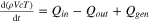
Figure 3 shows the heat transfer from the electrolyte with temperature Telect and the freeze with temperature Tfr to the anode with temperature Tan at the top. As two different thermal gradients exist, Kirchhoff's circuit laws are used by applying the electrical-resistance analogy, 38 and the equivalent thermal resistance circuit is represented in Fig. 4a. It can be further reformulated as Fig. 4b, so loops can be drawn and analysed. Relect−an is the thermal resistance due to convection between electrolyte and anode surface, Rfr is due to conduction from freeze to the anode surface, while Ran is due to conduction along the height of the anode. The formula for these resistances can be found in Table I. The solution to the thermal resistance circuit in Fig. 4b yields
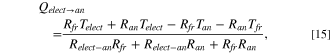

where Qelect→an and Qfr→an are respectively the heat transferred to the bottom anode surface from the electrolyte and the freeze, while Qelectfr→an is the total heat transferred up the anode.

Figure 3. Heat transfer to an anode from the surrounding electrolyte and freeze.
Download figure:
Standard image High-resolution image
Figure 4. (a) Equivalent thermal resistance circuit for heat transfer to the anode. (b) Rearranged thermal resistance circuit for heat flow calculations.
Download figure:
Standard image High-resolution imageHeat loss by anode
As Fig. 5 shows, the thermal energy lost from the top of the anode through the rod and yoke can be separated into two parts, since a portion of the assembly is hooded inside the cell and the rest is exposed to external potroom air. It is estimated that more than 45% of heat is lost through the top crust and anode, 19 amongst which 25% is lost through the stub and rod alone. Despite this, the stub and the rod were not considered in previously published spatial models.
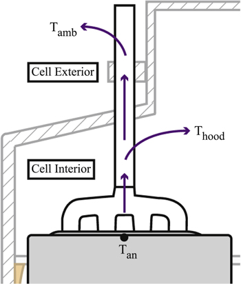
Figure 5. Heat loss through the rod and yoke of an anode
Download figure:
Standard image High-resolution imageThe thermal resistance circuit is represented in Fig. 6a, consisting of a parallel conduction network up the yoke, followed by conduction up the rod to midpoint of the assembly in the hooded environment. Some heat is lost by convection from the surface area of the internal yoke and rod to the hooded environment inside of the cell. The remaining heat energy conducts up the rod and is lost by convection to the ambient potroom air. Similarly, this circuit can be reformulated as Fig. 6b, where the R1 is the thermal resistance associated with conduction through the yoke and rod in the hooded environment, R2 is associated with heat convection to the hooded environment, and R3 is associated with heat conduction up along the rod to the portion outside of the cell, followed by heat convection to the potroom ambient air. The heat loss from the anode, Qan→hood,amb , is therefore given by one of the loops in Fig. 6b, which is

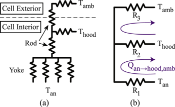
Figure 6. (a) Equivalent thermal resistance circuit for heat transfer from the yoke and rod. (b) Rearranged thermal resistance circuit for heat flow calculations.
Download figure:
Standard image High-resolution imageAdditionally, an industrial practice to mitigate carbon anode burnoffs involves dressing the top of the anodes with crushed frozen electrolyte materials. This is modelled with thermal conduction through the crust and convection to the hooded environment. 26 However, anodes that are newly-set are only dressed about 8 h into their service life, depending on operational procedures. Thus, dressing materials or top crusts are not found in new anodes, so are not included in the anode change model.
Heat balance around anode freeze
The freeze is modelled as an electrically-insulating cuboid that forms under a new anode in the entire interelectrode region, as the ACD is small relative to the anode dimensions. This cuboid changes dimensions as it dissolves back into the electrolyte, thereby exposing more surface area underneath the anode for electric conduction. The heat balances around an anode freeze are as follows:
- Vertical heat conduction from the centre of the freeze to the anode surface, Qfr→an .
- Heat convection from the metal pad below to the freeze, followed by vertical heat conduction to the centre of the freeze.
- The surfaces where the freeze contacts the electrolyte are at liquidus temperature. Heat from the electrolyte reaches this surface by convection, and leaves this surface for the centre of the freeze by conduction. The heat imbalance causes dissolution of freeze as shown in Eq. 10. 26
Therefore, the freeze shrinks only in the four sides that it interfaces with the electrolyte. It does not melt nor dissolve in the metal pad below, as the melting point of cryolite is higher than the operating temperature, and cryolite is not very soluble in aluminum. 39
An experiment was conducted to observe the freeze underneath new anodes. Newly-set anodes were pulled up three h into their service life, and the freeze observed was photographed from various angles for analysis. It was found that the four sides of the freeze dissolve at different rates, as shown by Fig. 7:
- The side facing the centre channel of the cell dissolves the quickest, aided by the extra electrolyte volume in the region and turbulence induced by bubbles from the opposing anode.
- The side facing the back wall of the cell dissolves slowly, as it is closest to the side ledge and experiences a large heat loss.
- In modern cell operations, anodes are set in pairs. The side facing the other new anode will also dissolve slowly due to the low temperature in the region.
- The remaining side that faces an older anode dissolves at a medium rate, owing to heat generation and bubble turbulence from the older anode.

Figure 7. (a) Anode freeze observed underneath an anode three h after change. (b) Surface underneath the anode covered by freeze, as obtained with image processing.
Download figure:
Standard image High-resolution imageThe dissolution rate also depends on the location of the anodes as well as electrolyte flow patterns. It can be modelled by using different HTC values for each side of the anode freeze.
Other heat balances
As summarised in Table I, heat transfer exists between other domains in the model:
- Alumina feed is introduced into the electrolyte with feeders along the centre channel of the cell as illustrated in Fig. 2. Near the feeding zone, energy is required to preheat the alumina feed to 960 °C and dissolve it in the electrolyte. The mass of alumina fed and dissolved comes from the mass balance, and the energy requirement per mass of alumina can be stoichiometrically calculated from the values provided in Table IV.
- Heat is transferred between the electrolyte regions by conduction as well as advection, due to its bulk flow.
- Similar to the anode freeze, there is convective heat transfer from the electrolyte to the surface of side ledge, and conductive heat from the surface into the midpoint of side ledge. The difference between the energy transferred governs the formation or dissolution of side ledge.
- There is heat conduction outwards from the ledge to the sidewall and shell. There are also heat conduction between similar subsystems, i.e. ledge-ledge, sidewall-sidewall, and shell-shell.
- Vertically, there is heat conduction from the metal through the bottom insulation layers to the shell. As the model is not discretised vertically, these are treated as thermal resistances.
- Finally there is convective heat transfer from the outer shell to the ambient air. Radiative heat transfer is accounted in the effective HTC for heat convection.
Spatially-discretised mass model
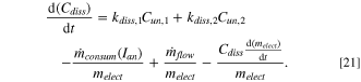
Alumina
Feeders in the cell consecutively dump alumina at a frequency determined by the feeding controller. Each alumina dump is assumed to have dispersed among the feeder zone and the eight subsystems surrounding it. A large portion of the alumina powder, r, dissolves quickly in the electrolyte, while the rest forms agglomerates that dissolve at a slower rate. 40 The dissolution of alumina in each of the subsystems around the feeding zone can therefore be modelled as a first-order model with 40


where Cun,1 and Cun,2 are the concentrations of solid alumina that dissolves at a rate of kdiss,1 (0.099 s−1) and kdiss,2 (0.005 s−1) respectively,
40
while  is the mass feeding rate of alumina with portion r (0.75) dissolving quickly. It is assumed that the alumina fed by the point feeder is dispersed among the four surrounding subsystems. In general, the mass balance of dissolved alumina in each subsystem depends on four components:
- Dissolution of alumina in the electrolyte (Eqs. 19 and 20).
- Consumption via process reactions (Eqs. 1 and 2). This is modelled with Faraday's law of electrolysis (Eq. 12).
- Advective mass transfer of alumina,
 , due to bulk flow of electrolyte (Eq. 5). The electrolyte velocities used in this study was provided courtesy of our industrial partner who performed computational fluid dynamics studies. Details of similar calculations can also be found in Feng et al.
41
and Zhu et al.
42
.
, due to bulk flow of electrolyte (Eq. 5). The electrolyte velocities used in this study was provided courtesy of our industrial partner who performed computational fluid dynamics studies. Details of similar calculations can also be found in Feng et al.
41
and Zhu et al.
42
. - Dilution as electrolyte mass increases due to the dissolution of freeze, or vice versa. This rate of change in electrolyte mass is given by Eq. 11.

Therefore, the mass balance equation for dissolved alumina in each subsystem is given by
Fluorides
Apart from alumina and cryolite, other electrolyte components include AlF3, CaF2, MgF2, LiF, and KF. Dissolution models similar to that of alumina can be considered for the fluorides, but the rate of fluoride loss from a cell is significantly less compared to alumina. With proper feeding of aluminum fluoride to compensate the loss of fluorides, it can be regarded that the net loss of fluorides is negligible. Therefore, the model can be simplified by considering only the advective mass transfer due to electrolyte flow and the changes in concentration due to evolution in freeze and ledge profile. Therefore, the mass balance of each fluoride species can be represented with an equation like the one below.

As aforementioned, the change in electrolyte composition affects the liquidus temperature. It is an important variable as the difference between electrolyte temperature and liquidus temperature, or superheat, represents the driving force for the formation or dissolution of freeze. The local liquidus temperature can be calculated with the empirical equation below: 43
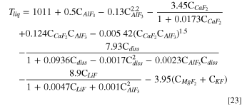
where Tliq is in °C and all the concentration terms in this equation are in wt%.
Anode-to-Cathode Distance (ACD)
The ACD is an important variable as it represents the interelectrode electrolyte resistance, which partially governs the amount of anode current flowing through the path, and therefore, local heat generation. There are four sources for the dynamics of ACD:
- Carbon anodes are consumed continuously during the reduction process, decreasing the anode height and increasing the ACD.
- Metal is produced and accumulated at the bottom of the cell during the reduction process, decreasing the ACD.
- After an anode change, the anodes and their assemblies, which were at ambient temperature, warm up considerably. Since the anodes are clamped and suspended in place at the rod (Fig. 5), any thermal expansion decreases the ACD.
- Beam movements as determined by a cell controller to maintain cell pseudo-resistance. Beam movements during metal tapping and anode raise events are not included, as these movements are done to maintain an overall ACD.
Therefore, the dynamic Eqs. for the anode height, Han , and ACD, D, are


where consum(Ian ) and accum(I) are the rate of anode height decrease and the rate of metal height accumulation respectively, which can be obtained from Faraday's law of electrolysis (Eq. 12). BM is the distance of beam moved due to cell control action, and expand(Tan ) is the vertical thermal expansion of the anode with its assembly. The typical thermal expansion formula only applies as an approximation for a linear expansion over a small temperature range. However, for a larger range and a varying thermal expansion coefficient expressed as AT + B, the new length of a material with initial temperature, T0, and initial length, L0, can be solved by integration, giving

where the thermal expansion coefficients for aluminum anode rods, steel yokes and stubs, and carbon anodes are provided in Table V. Initial lengths are also provided in the table but they are dependent on cell design.
Table V. Coefficient of Thermal Expansion.
| Material | A | B | Ref | L0 (cm) | T0 (°C) |
|---|---|---|---|---|---|
| Aluminium | 1.997 × 10⁻⁸ | 1.701 × 10⁻⁵ | 44 | 100 | 25 |
| Steel | 0 | 1.436 × 10⁻⁵ | 45 | 45 | 25 |
| Carbon | 2.709 × 10⁻⁹ | 2.9744 × 10⁻⁶ | 45 | 65 | 25 |
Finally, work practices also affect how the beam will be moved. During anode change, the beam is usually raised to increase the ACD, such that more heat will be generated to replenish the deficit energy caused by the changing of anodes. 46 New anodes are set also with ACDs that are a couple of centimetres higher than the old anodes they replace. This is mainly done in anticipation that the new anodes are consumed less as they are not carrying full current capacity.
Cell Voltage and Anode Current Distribution
As previously explained, the mass and thermal balance model can use actual measurements of cell voltage and anode currents, for applications such as simulating the local conditions of the cell. However, for simulation studies of behaviours of the local thermal variables, it is important to be able to compute the cell voltage as well as the anode current distribution.
The detailed and well-established cell voltage Eqs. have been published elsewhere, 32,47 so will not be repeated here for brevity. In short, cell voltage consists of the external voltage drop Vext , reversible potential EE , overpotentials arising from the alumina concentration gradient and the electrode surface reactions ηover , as well as the ohmic voltage drop due to electrolyte resistance Relect , bubble resistance Rbub , anode resistance Ran , and cathode resistance Rca . The general equation for cell voltage is given by

where C represents electrolyte composition and  is the total effective exposed anode area through which current flows. Virtually all the terms on the right-side of the equation are functions of temperature, and therefore they are not expressed as such for simplicity.
When the line current, I, is used for the computation,  is the sum of the bottom surface area of all the anodes. In the context of anode change, Eq. (27) is instead used with individual anode currents, while
  refers to the effective surface area of anode not covered by freeze. This includes any exposed area on the sides of the anode which allows any flowing current to fan out when the bottom surface is all covered. As the array of anodes in the cell are in an electrical parallel connection, the voltage through each path must be the same and all the anode currents must sum up to line current. Therefore, for N anodes, the anode currents and cell voltage at each time point can be computed by simultaneously solving
13
refers to the effective surface area of anode not covered by freeze. This includes any exposed area on the sides of the anode which allows any flowing current to fan out when the bottom surface is all covered. As the array of anodes in the cell are in an electrical parallel connection, the voltage through each path must be the same and all the anode currents must sum up to line current. Therefore, for N anodes, the anode currents and cell voltage at each time point can be computed by simultaneously solving
13
In this work, while the cell voltage equation considered traditional non-slotted anodes, slotted ones are also used in the industry for benefits such as reducing anode thermal stress and helping the release of gas bubbles from underneath the anode. 48 Slotted anodes are not considered in this work because calculations show that the electrolyte resistance dominates, as it is in the order of ten times larger than the bubble resistance. If included, the equation will also be highly empirical as there are many ways of slotting an anode, including different slotting orientations, widths, depths, angle of inclination, and profile. 48 This is outside the scope of this work, and we therefore consider that the bubble layer thickness and coverage is already representative for slotted anodes. Arkhipov et al. 49 have also found that slotted anodes have negligible impact on the anodic voltage drop.
Simulation Setup
Due to the coupling effects between process variables in this anode change model, Eqs. 3–28 have to be solved simultaneously. With suitable initial conditions, the numerical solution to the differential Eqs. can be found in Mathworks MATLAB®, giving the time-series value of the various process variables. The simulation starts after the freeze formation underneath both of the recently changed anodes.
Realistic initial conditions are used so the simulation results can be validated with measurements from an industrial cell. For example, the initial anode heights used are shown in Fig. 8; they are based on carbon consumption rate consum (Ian ), total anode service life, and anode replacement rota. This is so the distribution of anode current also reflects the anode resistance, and the thermal capacity and generation of each zone is realistic. The ACD, D, is initialised to 2.75 cm for all the anodes, except the new ones which are set 3 cm higher in this study. In this simulation, the alumina concentration is initialised with a value of 4.8 wt%, which is higher than the normal operating band. This is because firstly, the cell is overfed in preparation for the anode replacement to reduce the risk of anode effects, and secondly, lumps of crusts and other materials can fall into the electrolyte during the removal of spent anodes. 50 The initial undissolved alumina concentration is assumed to be zero; this value does not significantly change the results.
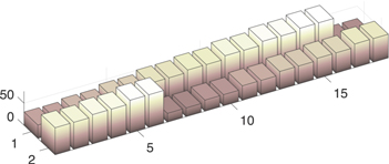
Figure 8. Height of the anodes in the simulated cell.
Download figure:
Standard image High-resolution imageThe different sides of the anode freeze that is in contact with the electrolyte will dissolve at varying rates subject to local thermal gradients and local cell conditions as previously explained. The latter can be modelled with different, but constant, HTC values for each face, since experiments have shown that a vertical freeze with gradual or steady dynamics does not significantly change the HTC. 51 The HTCs used for the cell studied are expressed as multiples of the nominal HTC between the electrolyte and the side ledge in Table VI.
Table VI. Assumed HTC between electrolyte and anode freeze at four sides for anodes 29 and 30.
| Position | HTC |
|---|---|
| Back wall | 1.5 helect−ledge |
| Centre channel | 10 helect−ledge |
| Facing older anode | 9 helect−ledge |
| Facing newer anode | 5 helect−ledge |
Experimental Setup
The industrial cell used for model validation has 36 anodes and 5 feeders, as shown in Fig. 9. Anodes 29 and 30 of this cell were replaced in an operation that started from 08:30 and lasted for more than half an hour, as the anodes had to be replaced one after another since the crane in this potroom is not capable of replacing both at once.

Figure 9. Layout of the industrial cell with 36 anodes and 5 alumina feeders (×). Anodes 29–30 are being changed. Electrolyte temperature measured at ⊙.
Download figure:
Standard image High-resolution imageProcess data collected includes individual anode currents, alumina feeding rate, electrolyte samples, and electrolyte temperatures. The last were measured at the tap-end, duct-end, between anodes 29 and 30 (new anodes), and between anodes 7 and 8 (opposite anodes), as indicated in Fig. 9. While measurements of anode current and feeding rates were automatically recorded at a frequency of 1 minute, the electrolyte samples and temperature measurements had to be manually taken. This was done by first breaking a hole in the crust to expose the electrolyte, and then waiting for a few minutes, as the materials that fell in would have affected the local process variables. The holes in the crust can close by themselves, and would have to be kept open by cell operators. The electrolyte samples were acquired hourly with a pair of preheated tongs, after which they were air-cooled and sent for laboratory analysis. The electrolyte temperatures were measured at a 15 min frequency with a mixture of Heraeus FiberLab TM and Marshall tip thermocouple TM due to limitations in measurement time and battery capacity of the FiberLab. A test-run was also conducted where both devices were simultaneously used at the same electrolyte location, and readings from both sensors were found to be consistent. Figure 10 shows the crust holes opened at the tap-end and between anodes 29–30, through which electrolyte samples or temperature measurements were taken.
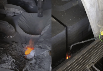
Figure 10. Photos showing the crust holes created in the tap-end and in the region of new anode to expose the electrolyte underneath. A probe with Marshall tip thermocouple is used to take the readings.
Download figure:
Standard image High-resolution imageResults and Discussion
In this section, the proposed model is validated by comparing its open-loop computations with real process data gathered from an industrial cell that was undergoing an anode change procedure.
Alumina concentration
As the dissolved alumina concentration is not continuously measured in an industrial cell, the commonly used "demand feed" algorithm 52 controls the alumina concentration within a band based on measurements of cell voltage and line current. In this algorithm, the feeding rate of alumina is cycled between over-feeding, base-feeding, and under-feeding, so the trajectory of cell voltage can be used to gauge the level of alumina concentration dissolved in the electrolyte. Although this feeding control algorithm has been added to the model such that feeding control actions can be completely simulated, the best way to validate the mass balance model is to use the actual feed rates from the industrial cell as model input.
Due to the feeding algorithm, feeder position, and the electrolyte flow, there will be spatial and temporal variations in the electrolyte. Figure 11 shows a heat map of the alumina concentration in the cell before anode change, immediately after, and 3 h after anode change. It can be seen that immediately after anode change, the concentration in the proximity of the new anodes is very high, since the electrolyte mass in those regions is assumed to drop dramatically due to rapid freezing. It is also observed that there is a difference in the distribution of alumina concentration before the anode change and 3 h after. One of the contributing factors is the redistribution of anode currents leading to different rates of alumina consumption at different locations.
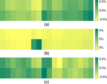
Figure 11. Heat map of dissolved alumina concentration as deviation from average initial percentage value (a) before anode change, (b) immediately after anode change, (c) 3 h after anode change.
Download figure:
Standard image High-resolution imageThe temporal variation can be validated by comparing the simulated and measured concentration level at the tap-end of the cell, as it changes according to the feed rate recorded from the industrial cell, as shown in Fig. 12.
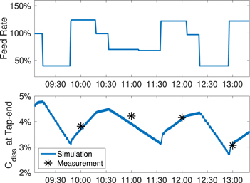
Figure 12. Alumina feeding rate and comparison of simulated and real alumina concentration at the tap-end.
Download figure:
Standard image High-resolution imageElectrolyte temperature
The electrolyte temperature also experiences spatial and temporal variations. Similar to the alumina concentration, Fig. 13 shows a heat map of the temperature distribution before, immediately after, and 3 h after the anode change operation. It is observed that while the electrolyte temperature before anode change is relatively even, the distribution changes very drastically after the operation with effects lasting for h. This again demonstrates how the anode change operation causes a massive disturbance to the thermal balance.
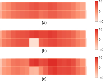
Figure 13. Heat map showing the temperature distribution as deviation from average initial temperature (a) before anode change, (b) immediately after anode change, (c) 3 h after anode change.
Download figure:
Standard image High-resolution imageIn order to validate the results obtained, the simulated and measured electrolyte temperatures at the tap-end, duct-end, between anodes 29–30, and between anodes 7–8 are compared in Fig. 14. The electrolyte temperature between anodes 29–30 is very low due to the deficiency in thermal energy caused by the cold anodes. The electrolyte temperature at the duct-end is also higher than at the tap-end, because the anodes are slightly older at the duct-end, and therefore are shorter with less resistance, assuming that they share the same ACD. Both the simulation and measurements show that the local electrolyte temperature can vary by as much as 13 °C. across the cell, which highlights the importance of having a distributed cell model, especially as superheat can be less than 10 °C. The oscillations observed in the electrolyte temperature are due to the cycling feeding rate shown in Fig. 12. The discrepancy in the duct-end electrolyte temperature in the first hour may be attributed to the changing electrolyte flow pattern upon the replacement of anodes 29–30, as it is observed that the measured temperature in the region remains high within the first hour, while a rising trend like that of the duct-end is expected. It is possible that the electrolyte flow at the duct-end may have temporarily changed as the freeze underneath anodes 29–30 impedes regular flow.

Figure 14. Comparison between simulated and measured electrolyte temperatures at the region of new anode, opposing anode, duct-end, and tap-end. Error bars represent uncertainties in the measurement.
Download figure:
Standard image High-resolution imageFreeze dissolution
Figure 15 shows how the freeze underneath one of the newly-set anodes dissolves away with time. As it dissolves, more of the anode is exposed, and the effective surface area increases. This allows more current to pass through, as shown in Fig. 16. Similar to our previous work, 23 it is observed that the new anodes do not reach full current carrying capacity when all the freeze has dissolved. Instead, the rate of anode current pickup decreases abruptly at around 6–7 h when all the freeze has disappeared, and from this point onwards, the anode current slowly approaches full capacity, taking a minimum of 4 days. 53 This is because even when the freeze has completely dissolved away, the path resistance is still greater because the new anodes have ACDs larger than the other anodes. This is consistent with Cheung's analysis of anode currents, 26 in which it was also noted that at this stage, these anodes behave like the other old anodes. Differences in ACD will eventually get rectified as it has a self-regulating behavior—as the currents through these anodes are less than the other anodes, less carbon is consumed and ACD will decrease at a greater rate compared to the other anodes.

Figure 15. Anode 29: A series of diagrams showing the simulated dissolution of freeze at different rates from four sides. (BW = back wall, CC = centre channel).
Download figure:
Standard image High-resolution image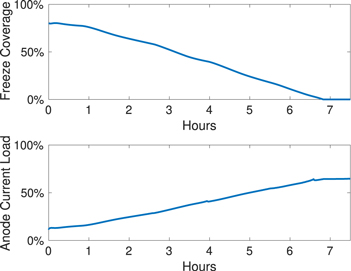
Figure 16. Anode 29: percentage of effective anode area covered by the freeze, and the amount of current flowing through the anode.
Download figure:
Standard image High-resolution imageThe freeze dissolution time will differ depending on cell technology, anode location, and local heat transfer conditions. In Cheung's work, 26 it takes on average around 6 h to reach full dissolution, with a standard deviation of 2.7 h. In order to illustrate this effect, another simulation is carried out where anodes at the cell corners (anodes 17–18) are changed instead. Parameters across the simulations are kept very similar to demonstrate just the effect of local heat conditions on the dissolution rate of the anode freeze. Hence, the same HTC as shown in Table VI are used, despite the likelihood that they will change according to anode location and electrolyte flow pattern. The only other difference is in the anode initial heights, since they should reflect the condition when anodes 17 and 18 are changed. The result is shown in Fig. 17; not only does the rate of freeze dissolution differ from the previous simulation study, but the freeze below the two anodes even dissolves at different rates. The freeze below anode 18 dissolves very slowly since it experiences greater heat loss and superheat is low in the area, as this anode is adjacent to two cell walls and more side ledge.
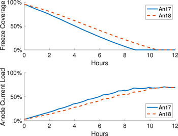
Figure 17. Alternate simulation replacing Anodes 17-18 (Corner anodes): Freeze dissolution rate differs for two anodes set simultaneously.
Download figure:
Standard image High-resolution imageThe results obtained are indirectly validated by comparing the simulated and measured current passing through anode 29 as it slowly picks up over several h, as shown in Fig. 18. Minor differences in the trajectories include the initial anode current load. This is because this model assumes that at the beginning, pieces of freeze at the sides of the anode have already broken off, and therefore has exposed some surface area for electricity conduction. Meanwhile, the bumps in anode current observed at around 11:30 and 14:30 are due to known and unrelated process disturbances elsewhere in the cell.

Figure 18. Anode 29: Comparison between simulated and measured anode current.
Download figure:
Standard image High-resolution image
This validation demonstrates that with suitable parameters and initial values, the model can be used to predict and study the overall trends of anode current distribution and local cell dynamic response during and after an anode change procedure. When the model is implemented online with feedback from actual process measurements like anode currents and cell voltage, process parameters and initial values can be recursively identified in real-time using online estimation techniques such as an Extended Kalman Filter 54 to achieve higher accuracy in the prediction of future process variables.
However, implementation of feedback-based correction is outside the scope of this paper, which focuses on the process mechanisms and model structure; process parameters vary across different cell technologies.
Conclusions
A coupled mass and energy balance model has been developed to describe the dynamics in local cell process variables and redistribution of anode current following an anode change operation. This integrated model accounts for the interactions between mass and thermal variables, for example, changes in electrolyte mass caused by the dissolution of freeze, which in turns affects heat generation. The model is spatially-discretised to capture dynamics in local process variables, and it has been shown that spatially, alumina concentration can differ up to 1 wt% and electrolyte temperature can vary by more than 10°C across the cell. This model is also generic and applies to a wide selection of prebaked cells, as differences in cell designs are accounted by model parameters. Experimental validation with electrolyte samples, electrolyte temperature measurements, and anode current measurements from an industrial cell undergoing anode change shows that the model can be used to predict the trends in local variables.
It is shown that anode change has a significant impact on the mass and thermal balance which will then negatively affect process efficiency. As the proposed model fills in the knowledge gap in aluminum reduction cell modelling, it can be used to improve operations and control which can minimize this impact of this operation. For example, it can be used to study the replacement of new anodes at unconventionally low ACD to limit the amount of freeze formed, which can increase the speed of anode current uptake. Another example is that the integration of the proposed model will allow other model-based monitoring and control techniques to be much more complete and more useful across the routine operations. More studies can be conducted with the model to optimize the anode change operation, which involves making the optimum control and operative decision for each anode location, such as alumina feeding rate and the height at which new anodes are placed. The optimum rates of freeze dissolution and current pickup can also be investigated. All of these will increase process efficiency, decrease energy consumption, and reduce emissions, which is the key to the scalability of the industry for the next few decades.
Acknowledgments
This project was supported by the Emirates Global Aluminium (EGA) and Australian Research Council (ARC) Research Hub IH180100020. The technical support from the EGA, Jebel Ali Operations are also gratefully acknowledged.