

Abstract
Electrochemical Impedance Spectroscopy was utilized to investigate the corrosion behavior of carbon steel in a salt spray test (SST) chamber. The salt spray was applied using 5% NaCl solution at 35 °C. A two-electrode cell comprising a pair of identical carbon steel electrodes embedded in epoxy resin were placed at six different angles (0°, 30°, 45°, 60°, 75°, and 90°) to the horizontal in the chamber. The corrosion rate (CR) of the carbon steel samples and the thickness of the solution film formed on the sample surface were evaluated from the impedances at low and high frequencies, respectively. The CR of carbon steel fixed horizontally (0°) exhibited a low value compared with that fixed at other angles. When the angle changed from 30 to 75°, the solution film thickness decreased greatly, but there was no significant difference in the CR. The CR of carbon steel under the employed SST conditions was more than five times higher than that in a bulk 5% NaCl solution under natural convection. The corrosion mechanism of carbon steel in the SST chamber is also discussed.
Export citation and abstract BibTeX RIS
Steel materials are applied in a wide range of fields due to their excellent mechanical properties, workability, and weldability. However, their susceptibility to corrosion in atmospheric environments, when used without paints, is a problem. This resulted in the development of corrosion-resistant steel, such as weathering steel. To develop corrosion-resistant steel materials and evaluate their corrosion resistance, several accelerated corrosion tests, such as the salt spray test (SST) and the cyclic corrosion test (CCT), are widely used. Such accelerated tests are preferred over long-term outdoor exposure tests in the development and selection of materials because of the convenience of reduced time required for the testing. For such accelerated corrosion tests, the test specimens are placed in a test chamber for a certain period of time and then evaluated on the basis of changes in appearance and/or amount of corrosion that are calculated from the thickness and/or mass losses observed after the tests. However, the results from accelerated tests frequently disagree with those acquired after long-term exposure tests in real atmospheric conditions. Moreover, in the case of tests such as CCT, one cycle comprises several steps such as salt spraying, drying, and wetting, and the way various phenomena occurring at each step affect the total corrosion values is not always understood. Therefore, corrosion monitoring is necessary during accelerated tests.
Several methods have been studied for monitoring the changes in corrosion rate (CR) due to environmental changes. The quartz crystal microbalance (QCM) method, based on the fact that the resonance frequency of a crystal unit changes with the change in mass due to corrosion, has been utilized for the monitoring of indoor corrosion.1–3 The method has a detection sensitivity of 1 to 10 ng cm−2 and can measure minute CRs that cannot be otherwise detected in exposed test specimens. Hosoya et al. applied QCM to measure the amounts of sea salts deposited on carbon steel and iron surfaces, and examined the effects of the composition and thickness of water films on their atmospheric CRs.3 This technique is very powerful for detecting trace amounts of corrosion such as that seen in the indoor corrosion of electronic components, but unsuitable for environments with a relatively high CR, such as during outdoor corrosion and accelerated tests.
An electric resistance (ER) technique has been also used for corrosion monitoring. This method quantifies the CR by measuring the increase in resistance of the material itself due to its thinning by corrosion. In recent years, suitably modified ER sensors have also been developed and used for monitoring atmospheric corrosion,4–6 as well as for corrosion monitoring in accelerated corrosion tests.7,8 ER is a very good method for atmospheric corrosion monitoring; however, to measure the CR of a material, it is necessary for the sensor material to be thin because the optimum thickness of a sensor depends on the CR and, therefore, thinner sensors are required for measuring relatively slow CRs. In other words, it is not possible to directly measure the CR of bulk material.
Electrochemical impedance spectroscopy (EIS) is another powerful method to monitor the corrosion of metallic materials in various environments9–25 because of its ability to estimate instantaneous CRs. This method offers the advantage of allowing bulk materials to be used as working electrodes (corrosion monitoring sensors). Nishikata et al. employed EIS for the first time to measure the CR of metals under a thin solution film (to mimic atmospheric corrosion), and successfully described its behavior by using a transmission line (TML)-type equivalent circuit.11 The method has also been successfully employed to monitor the corrosion of carbon and weathering steel samples exposed to many actual atmospheres.14 Therefore, applying this corrosion monitoring system to accelerated corrosion testing should provide valuable information for understanding the differences in corrosion behavior from in actual atmospheres. We are considering applying this monitoring system to CCT, which is an accelerated test of atmospheric corrosion. As a first step, in this study, we applied it to monitor the corrosion behavior of carbon steel in SST because salt spray is an important step in CCT. Special attention was paid during the SST to the effect of exposure angles on the corrosion of the carbon steel, as the solution film thickness has a significant effect on the CR.12
Experimental
Electrochemical cell
The corrosion monitoring was performed under SST conditions by using an EIS setup with a two-electrode cell, as shown in Fig. 1a. Carbon steel (SM490) plates of four different sizes, 10 mm × Xw (0.2, 0.5, 1, and 10 mm), were used as specimens. The chemical composition is shown in Table I. For the cell, a pair of identical carbon steel plates were embedded in epoxy resin with a gap of Xg = 50 μm. The cell surface was polished with emery papers up to #600 grade and then ultrasonically cleaned in ethanol.

Figure 1. Schematics of the electrochemical cell for measurements of (a) electrochemical impedance spectroscopy and (b) solution resistance.
Download figure:
Standard image High-resolution imageTable I. Chemical composition of carbon steel (SM490) (wt%).
| C | Si | Mn | P | S | Fe |
|---|---|---|---|---|---|
| 0.16 | 0.22 | 1.05 | 0.025 | 0.004 | Bal. |
SST
The corrosion test was conducted by using an SST instrument (Suga Test Instruments Co., Ltd model CASSER-IIR-ISO-3 type). The electrochemical cells for EIS measurements and the coupon specimens for mass loss measurements were placed in the SST chamber. A 5% NaCl solution was sprayed on the cell and the specimen surfaces with 0.093 MPa of atomizing over pressure at 35 °C.
EIS measurement
The EIS measurements were taken in situ during the SST using the cell depicted in Fig. 1 with an electrochemical unit (Solartron 1280B), at an AC voltage amplitude of 10 mV and a frequency range of 10 kHz to 10 mHz. The obtained EIS was analyzed with a software (Scribner Associates, Inc. ZView version3.5e). In EIS measurements under a thin solution film, the current distribution over the electrode should also be considered,11 and the width of the electrode (Xw in Fig. 1) is an important factor in determining this current distribution. First, to determine the optimum electrode size, EIS measurements were obtained from the SST chamber using four electrochemical cells, each containing an electrode of different width (Xw = 0.2, 0.5, 1, and 10 mm), with the cells placed at an angle of 75°. Later, using measurements obtained from the cell with the optimum electrode size, the corrosion behavior of carbon steel was investigated by using EIS. Special attention was paid to the angles at which the cells were fixed: 0° (horizontal), 30°, 45°, 60°, 75°, and 90° (vertical). The corrosion test duration was 24 h.
Corrosion mass loss measurement
Using the same carbon steel type as that used in the EIS measurements, the average CR of a plate (50 mm × 50 mm × 2 mm) was determined by measuring the mass loss after a 24 h exposure to salt spray. For this test, the specimen surface was first ground to #600 grit finish using SiC papers. The specimens were then mounted on 70 mm × 150 mm × 2 mm polyvinyl chloride boards. The exposure angles of the specimens were 0°, 30°, 45°, 60°, 75°, and 90° to the horizontal, same as those used in the EIS measurements. The test duration was 24 h. The rust was removed by the immersion in solution of 10% diammonium hydrogen citrate C6H14N2O7 + 0.3% inhibitor (Asahi Chemical Co., Ltd, IBIT No. 30AR).
Estimation of solution film thickness
The average solution film thickness Xf at each exposure angle was roughly estimated by measuring the solution resistance Rsol between the gap distance of the two electrodes by EIS, assuming that a uniform liquid film was maintained on the electrode surface under SST. For Rsol measurement, a two-electrode cell shown in Fig. 1b was employed, with electrodes of 10 mm × 0.5 mm (Xw = 0.5 mm) dimensions, and with a gap of 10 mm between the two electrodes. To accurately measure the Rsol value, we employed electrodes with a smaller Xw and a larger gap than in those used in the corrosion monitoring cell (Fig. 1a). The surface of the electrode cell was ground to #600 grit finish using SiC papers.
The relationship between the Rsol and Xf values of the cell of Fig. 1b was obtained in advance as follows. The 5% NaCl solution films of various thicknesses, with the same concentrations as used in the SST, were laid on the horizontally fixed cell surface in a chamber at 35 °C. Rsol was obtained from the impedance at 10 kHz. The Xf value was calculated from the volume of the solution film placed on the cell surface, assuming that the shape of the solution film can be approximated by a disk with a diameter of 30 mm (=diameter of epoxy resin), since Xf (100 μm ∼ 2 mm) of the solution film employed was sufficiently smaller than the diameter. Using the obtained relation between the Rsol vs Xf, the Xf value for each angle of the electrode in the SST was roughly estimated from the monitored Rsol during SST.
Results and Discussion
Optimum electrode size
Figure 2 shows the EIS measurements after 24 h exposure in the SST chamber using cells with the four different Xw values exposed at 75°. Note that the absolute value of impedance Z is not normalized by the electrode surface area, as it may be necessary to consider non-uniform current distribution. The electrode and solution film interface can be expressed by a one-time constant equivalent circuit comprising the solution resistance in series with a parallel circuit of charge transfer resistance Rct and double layer capacitance. In this equivalent circuit, Rct is given by the impedance at the low frequency limit ZLow and the reciprocal of Rct is proportional to the corrosion current icorr.26 Accordingly, for all the electrodes illustrated in Fig. 2, the converted value of ZLow (Ω cm2) value per unit surface area must be equal. Indeed, it can be observed that the converted ZLow (Ω cm2) values at 10 mHz for Xw = 0.2, 0.5, or 1 mm are almost equal. However, the converted ZLow (Ω cm2) value for Xw = 10 mm is approximately four times larger, which means that at the low frequency limit, the current was evenly distributed for Xw values of 0.2, 0.5, or 1 mm, whereas it was unevenly distributed for Xw = 10 mm. The current distribution can be evaluated from the phase shift θ because it strongly depends on the frequency.11,12,15 As the frequency increases, the current tends to concentrate near the edges between the two electrodes (Fig. 1), and as the frequency decreases, the current becomes more evenly distributed over the electrodes. In the previous papers,11,12 it was reported that when the θ exceeds 45° at a certain frequency fcrit, the current distribution changes from non-uniform to uniform at the fcrit. In a lumped constant equivalent circuit with uniform current distribution, the impedance Z can be expressed as Z ∝ exp (jθ). In this case, θ varies from 0 to 90 °. On the other hand, Z is given by Z ∝ exp (jθ/2) in a 1D distributed constant equivalent circuit with non-uniform current distribution. In this case, θ varies from 0 to 45 °. Therefore, if θ exceeds 45 °, the current will be evenly distributed over the electrodes. It can be observed from Fig. 2 that θ exceeds 45° except for Xw = 10 mm. This indicates that the current distributions for Xw = 0.2, 0.5, and 1 mm became uniform in the lower frequency region than the fcrit and an accurate Rct can be obtained from ZLow. Conversely, in case of Xw = 10 mm, it indicates that the current was unevenly distributed at the low frequency limit because the θ value was smaller than 45° in the whole frequency region. Thus, in case of Xw = 10 mm, icorr will be underestimated if ZLow is assumed as Rct.
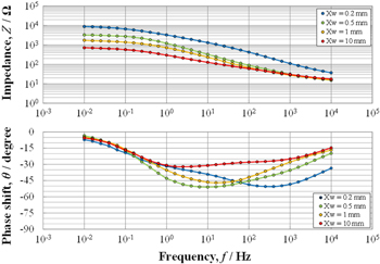
Figure 2. EIS readings of carbon steel measured at the corrosion potential in the SST chamber using the electrochemical cells described in Fig. 1a. The symbols and lines are the experimental and fitting results, respectively; Xw = 0.2, 0.5, 1, and 10 mm; exposure angle = 75°.
Download figure:
Standard image High-resolution imageIn case the solution film thickness over the electrodes is very less, as in the SST environment, a TML equivalent circuit that takes into account the current line distribution should be used to determine Rct.11,15 The TML equivalent circuit is shown in Fig. 3, where, Xw: width of the electrode in Fig. 1; Rct*: charge transfer resistance per unit length; CPE*: constant phase element per unit length; Rs*: solution resistance per unit length; and Rsol: solution resistance between the two electrodes. The results of curve-fitting the EIS data to the TML are represented by the lines in Fig. 2. It is evident that the fitting curves are in good agreement with the experimental data (symbols). The obtained parameters from the curve-fitting are summarized in Table II. The obtained Rct value for Xw = 10 mm almost accorded with that for Xw = 0.2, 0.5, or 1 mm.

Figure 3. Transmission line type equivalent circuit. Xw: width of electrode in Fig. 1a; Rct*: charge transfer resistance per unit length; CPE*: constant phase element per unit length; Rs*: solution resistance per unit length; Rsol: solution resistance between two electrodes.
Download figure:
Standard image High-resolution imageTable II. Parameters used in the equivalent circuit of Fig. 3.
| Xw | Rsol /2 | Rct* | CPE* | α | Rs* |
|---|---|---|---|---|---|
| (mm) | (Ω) | (Ωcm) | (F cm−1s(α−1)) | (Ω cm−1) | |
| 0.2 | 7 | 188 | 0.0026 | 0.57 | 1.8E-07 |
| 0.5 | 13 | 185 | 0.0027 | 0.77 | 3.6E-02 |
| 1 | 14 | 184 | 0.0019 | 0.89 | 9.2E-02 |
| 10 | 12 | 186 | 0.0077 | 0.79 | 2.7E + 03 |
As mentioned above, an accurate Rct can be obtained by curve-fitting the obtained EIS data to the TML equivalent circuit, even if large electrodes (large Xw) are employed. However, the curve-fitting becomes extremely difficult if the current distribution is significantly concentrated on the near edges between the two electrodes, and if the electrode surfaces are covered with thick rust layers. To save time, the impedance observed at 10 mHz was adopted as Rct without curve-fitting and by using a smaller electrode.
From the viewpoint of current distribution, a smaller electrode is better. However, if Xw is smaller than the solution film thickness Xf, the oxygen diffusion through the solution film changes from one-dimensional to two-dimensional, which may accelerate the CR. In addition, smaller electrodes increase the external noise during EIS measurement. Thus, Xw = 0.5 mm was selected as the optimum electrode size.
EIS characteristics
Based on the above discussed examination, electrochemical cells with Xw = 0.5 mm and Xg = 0.5 mm were fabricated, and EIS measurements were obtained at cell exposure angles of 0° (horizontal), 30°, 45°, 60°, 75°, and 90° (vertical) in the SST chamber. Figure 4 shows the EIS measurements after 24 h of exposure. Comparing the high-frequency impedance at 10 kHz (Z10kHz), the horizontal installation (0°) displayed the smallest value probably because the solution film covering the surface was the thickest. For the cell angle range of 0°–60°, Z10kHz increased with the angle because the solution film became thinner and the value decreased even more with a further increase in the angle from 75° to 90°. Z10kHz increased in the order Z(0) < Z(30) = Z(75) < Z(90) < Z(45) < Z(60), but there were no significant differences. The details are discussed in later sections.
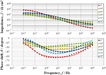
Figure 4. EIS measurements of the electrochemical cells given in Fig. 1b exposed at different angles (0°, 30°, 45°, 60°, 75°, 90°) in the SST chamber.
Download figure:
Standard image High-resolution imageThe current distribution on the electrode was evaluated with θ. As θ at 0°, 75°, and 90° exposure angles exceeded 45°, it can be concluded that the current distribution is uniform at the low frequency limit. On the other hand, θ at 30°, 45°, and 60° exposure angles did not exceed 45°. This is not due to the onset of uneven current distribution, but rather to the formation of a thick rust. If the CPE parameter α is unity, the critical phase shift θcrit required for judging whether the current is even or uneven is 45°. In other words, if θ exceeds 45°, the current distribution will be uniform at the low frequency limit, otherwise it will be considered non-uniform. However, if α is smaller than 1, the θcrit value decreases as α is smaller.27 In the EIS values shown in Fig. 4, as the electrode surface was covered with a thick rust, the value of α should be significantly small and θcrit is expected to be significantly lower than 45°. As will be shown later, the CRs estimated from the impedance at 10 mHz (≈ Rct) and from corrosion mass loss values agree very well. Therefore, it can be concluded that the current distribution in the low frequency limit was uniform at all angles.
In this study, the impedance at 10 mHz was taken as the charge transfer resistance Rct. The corrosion current density icorr (A cm−2) at each angle was estimated with the Stern-Geary equation (Eq. 1) by using Rct (Ω cm2) and a proportional constant k of 20 mV,28

Then, the icorr value was converted into the CR (mm y−1). The CR observed after 24 h of exposure was 0.36 mm y−1 at 0°, 2.53 mm y−1 at 30°, 2.45 mm y−1 at 45°, 1.77 mm y−1 at 60°, 1.83 mm y−1 at 75°, and 1.12 mm y−1 at 90°. The CR of horizontally fixed carbon steel was the lowest, the CRs for specimens at 75° and 90° angles were the next lowest, and the CRs for 30°, 45°, and 60° were similar. The CR in the SST chamber seemed to be significantly higher than that in the bulk NaCl solution under static conditions. The details of the corrosion mechanism are discussed in a later section.
Surface appearance and corrosion mass loss
To measure the corrosion mass loss at the same cell angles as those used for the earlier tests, coupon specimens created from the same carbon steel as that constituting the electrodes were fixed on polyvinyl chloride boards in the SST chamber. After 24 h exposure, the coupons were removed from the chamber, the photos of the surface appearance were taken, and then the corrosion mass loss was measured after removing the corrosion products.
The surface appearance at different angles is shown in Fig. 5. It can be seen that the corrosion morphology is significantly different for various exposure angles. The specimen surface exposed at 0° (horizontal) angle was completely covered with a relatively thin red rust. It was visible from the amount of corrosion products that the CR was much lower than that for the other angles (30°–75°). The surfaces at 30° and 45° angles were partially covered and almost completely covered with thick red rust at 60° and 75°, with a striped form. Probably, during the SST, the solution film drifted downward on the surfaces at 30–75° angles. On the surface exposed at 90° (vertical) angle, several dots of red rust were observed, where the solution may have remained in the form of droplets. The different morphologies may have resulted from the different states of the solution film on the specimen surfaces.

Figure 5. Surface appearance of the coupon specimens after 24 h of exposure at different angles in the SST chamber. (a) 0°, (b) 30°, (c) 45°, (d) 60°, (e) 75° and (f) 90°.
Download figure:
Standard image High-resolution imageFigure 6 shows the average CRs determined from the corrosion mass loss of specimens exposed at different angles during 24 h of exposure in the SST. The specimen fixed horizontally (0°) had the lowest CR of approximately 1 mm y−1. The CR of the specimen fixed vertically (90°) was the second lowest (approximately 1.5 mm y−1). The CRs for specimens fixed at 30°, 45°, 60°, and 75° were similar (approximately 2 mm y−1). The CRs calculated from the Rct value are also shown in Fig. 6. The tendency of the angle dependency agreed well between the mass loss and EIS results. The absolute CR values for all angles were similar except for 0°. The CR determined with EIS was less than half of that calculated from the mass loss at 0°. Notably, the CR obtained from the mass loss observations is the average value for 24 h SST, whereas the CR obtained from EIS measurements is the instantaneous rate observed just at the completion of 24 h exposure, which suggests that the CR decreased with exposure time at 0° and did not change with time at the other angles.

Figure 6. Corrosion rate plots of carbon steel vs exposure angle determined from corrosion mass loss and charge transfer resistance.
Download figure:
Standard image High-resolution imageSolution film thickness
The Rsol measurements with the cell described in Fig. 1b are shown in Fig. 7. At angles of 0°, 30°, 45°, 60°, and 75°, the Rsol value declined rapidly during the initial 3 ∼ 5 h and then reached a steady state. This decrease is due to the surface wetting by the salt spray. On the other hand, at 90°, Rsol fluctuated greatly during monitoring, indicating that the solution film was unstable in a vertical position. Therefore, vertical exposure was excluded from the analysis of solution film thickness.

Figure 7. Changes in solution resistance with time as a function of exposure angle.
Download figure:
Standard image High-resolution imageFigure 8 shows the relation between Rsol and Xf measured for samples with thicknesses ranging from 200 to 2000 μm, using the cell described in Fig. 1b. The dotted line in the figure is the result obtained from the electrical conductivity (к = 0.086 S cm−1)29 of 1 M NaCl (5.9%) solution at 25 °C. For the calculation, the length, width, and height of the solution were 1 cm, 1 cm, and Xf, respectively (Fig. 1b). As shown in Fig. 8, the measured points are on the dotted line when the solution film is thick, but deviate from the dotted line for a thin film. At this point, the deviation cannot be clearly explained, but using this standard curve, the thicknesses of the solution films in SST, estimated roughly from the Rsol values at 6 h in Fig. 7, were obtained as approximately 3000 μm at an exposure angle of 0°, 500–600 μm at 30°, 100 μm at 45°, and 60 μm at 60°. It may be difficult to estimate it at 75° because Rsol (approx. 2 × 10⁴ Ω) at that angle was significantly out of the standard curve range. Assuming that there is a linear relationship between Rsol and Xf on the thinner side of the film, the extrapolation of the straight line provides an estimate of a few tens of a micrometer for Xf.

Figure 8. Relationship between solution resistance and solution film thickness determined by using the cell described in Fig. 1b.
Download figure:
Standard image High-resolution image
Corrosion mechanism
It is well known that the corrosion of carbon steel in a neutral environment proceeds by following a combination of anodic iron dissolution reaction (Eq. 2) and oxygen reduction reaction (Eq. 3).


The rate-determining step (rds) of the corrosion process is the oxygen diffusion. During the atmospheric corrosion of carbon steel, the rate of oxygen reduction reaction (ORR) is controlled by diffusion through a solution film on the surface. Nishikata et al. have also previously reported on atmospheric corrosion mechanism.12 When the solution film reaches a thickness of approximately 300 μm or more, the CR is independent of Xf. This is because the thicker solution film is composed of two layers: an inner diffusion layer and an outer convection layer. An increase in Xf only increases the convection layer thickness. On the other hand, a solution film thinner than approximately 300 μm is composed of only a diffusion layer, and a decrease in Xf promotes the diffusion of oxygen. The CR increases almost proportionately to the reciprocal of the solution film thickness (Xf−1).12 However, the CR shows a maximum value of a few tens of a micrometer, and when the solution film is further thinned, the CR starts to decrease. It is considered that this decrease may be due to the fact that the rate of anodic dissolution reaction (Eq. 2),30 that is, the ionization reaction of Fe, is strongly suppressed. Simultaneously, when Xf is a few tens of a micrometer or less, the rds of the ORR also changes from being a diffusion process in the solution film to being a dissolution process of oxygen molecules at the air/solution film interface. Thus, the ORR rate becomes independent of Xf.12
The corrosion mechanism in SST should be considered from the point of view of its dependence on the solution film thickness. It is clear from the Rsol results given in Fig. 7 that Xf changes by changing the exposure angle. Conversely, looking at the dependence of the CR on the exposure angle in Fig. 6, Xf is approximately 3 mm at 0° (horizontal) from Fig. 8, and the CR is the lowest among all the angles (approx. 1 mm y−1). For the other angles, Xf was roughly estimated to be 500–600 μm at 30°, approximately 100 μm at 45°, 60 μm at 60°, and a few tens of a μm at 75°. Although Xf seemed to have changed greatly, the CR exhibited an almost constant value of roughly 2 mm y−1. The dependence of CR on Xf during the SST was different from that under static solution film conditions.12 This may be attributed to differences in the way oxygen is supplied to the specimen surface; that is, under static conditions, oxygen is supplied to the specimen surface by diffusion through the solution film, whereas in SST, fresh oxygen-containing solution is constantly supplied to the specimen surface. This suggests that in SST, the diffusion process of oxygen through the solution film is not completely rate-determining. In other words, the dependence of the CR on Xf in SST is lower than that in stationary solution film test. This can also be confirmed from the fact that the obtained CR in SST was significantly higher than that under static conditions. For example, the horizontal specimen set had an average CR of 1 mm y−1, which was the lowest among all angles. The horizontal specimen was covered with an approximately 3 mm-thick solution film of 5% NaCl in SST. If a 3 mm-thick solution film is present on the surface in a static condition, the CR should be almost the same as that in a bulk solution under natural convection.29 The CR of carbon steel in 5% NaCl solution at 35 °C for 24 h was determined as 0.19 mm y−1 after mass loss measurement. It is evident that the CR of carbon steel under the employed SST conditions was more than five times higher than that under the stationary system, which means that there is an extremely high supply of oxygen to the specimen surface in SST.
In the above corrosion mechanism, the effect of rust was not considered. The low angular dependence of CR and accelerated corrosion can also be explained by the formation of rust, if FeOOH acts as the main oxidant of steel corrosion. In CCT, which includes a drying step in each cycle, electrochemically active FeOOH is formed in the drying step and promotes corrosion by acting as a strong oxidant in the subsequent wetting step.31,32 Also, since the main oxidant changes from O2 to FeOOH, the CR may be independent of the solution film thickness. However, in SST without the drying step, it may be difficult to form active FeOOH because the sample surface is always wet.
Conclusions
The corrosion behavior of carbon steel fixed at different angles (0°, 30°, 45°, 60°, 75°, and 90°) in an SST chamber at 35 °C was studied through EIS and corrosion mass loss measurements, and the following conclusions were derived.
- 1.The optimum size of electrode width for the EIS measurement was determined to be 0.5 mm, considering the current distribution on the electrode, oxygen diffusion through the solution film, and external noise.
- 2.The corrosion rate estimated from the charge transfer resistance measured through EIS agreed well with that obtained through mass loss. In the SST chamber, the corrosion rate was successfully measured with EIS. The solution film thickness on the SST test piece was roughly estimated from the solution resistance determined by using EIS.
- 3.The corrosion rate was the lowest in horizontally fixed carbon steel (0°). There was no significant difference in the corrosion rates at 30° and 60°, although the solution film thickness changed considerably.
- 4.The corrosion rate of carbon steel under the employed SST conditions was more than five times higher than that observed in an NaCl bulk solution under natural convection.