Modeling Overcharge at Lithiated-Graphite Porous Electrodes: Plating and Dissolution of Lithium

Daniel Baker; Mark Verbrugge

doi:10.1149/1945-7111/ab90ab

List of symbols

${a}_{s}=\tfrac{3{\varepsilon }_{1}}{a}$	Surface to volume ratio of porous electrode, 1/cm
$a$	Spherical particle radius in porous electrode, cm
${a}_{Li},{a}_{H,j},{a}_{j}$	Activities of plated lithium, unoccupied and occupied sites of gallery j of the graphite
${c}_{2}$	Salt concentration in liquid phase, mol cm⁻³
${c}_{0}$	Value of ${c}_{2}$ at equilibrium, mol cm⁻³
${c}_{T}$	Maximum concentration of lithium in electrode, mol cm⁻³
$D$	Diffusion coefficient in solid phase, cm² s⁻¹
${D}_{2}$	Diffusion coefficient in liquid phase, cm² s⁻¹
${f}_{\pm }$	Activity coefficient of electrolyte salt
$F$	Faraday constant, Coulomb mol⁻¹
${i}_{1},{i}_{2}$	current density in the solid or liquid phase, A cm⁻²
${i}_{0,j}^{ref}$	exchange current density, gallery j of graphite A cm⁻²
${i}_{0,j}$	See Eq. 6, A cm⁻²
$I$	Total current density at 1-C rate
${j}_{1},{j}_{2}$	Current density of lithium insertion or lithium plating reactions, A cm⁻²
$L,{L}_{sep}$	Width of porous electrode or separator, cm
$Q$	Specific (volumetric) amount of plated and intercalated lithium, C cm⁻³
$\bar{Q}=\tfrac{Q}{F{c}_{T}{\varepsilon }_{1}}$	Dimensionless total charge of intercalated plus plated lithium, Eq. 17
${r}_{T}$	Reaction rate of reaction 13, see also Eq. 16, mol cm⁻²-s⁻¹
$r$	Radial coordinate in spherical particles, cm
$R$	Gas constant, J cm⁻³-K⁻¹
$\begin{array}{l}{R}_{e},{R}_{s},{R}_{e,diff},{R}_{sep}\\ {R}_{d},{R}_{k},{R}_{Li},{R}_{1-2}\end{array}$	Electrode resistances, see Eq. 37, Ohm-cm²
$s$	transformation variable, Eq. 25
$t$	Time, s
${t}_{0}$	Diffusion time ${a}^{2}/D,$ s
${t}_{+}^{0}$	Transference number
$T$	Temperature, K
${U}_{1}$	Open circuit voltage of intercalation reaction, V
${U}_{2}$	Open circuit voltage of plating reaction
${U}_{j}^{0}$	See Eq. 2, V
$V$	Electrode voltage with respect to a lithium reference, V
$x,{x}_{j},{x}_{H,j}$	Total mole fraction of lithium, occupied and unoccupied site fraction in solid phase, respectively
${X}_{j}$	Maximum mole fraction of species j, see Eq. 2
$z$	Coordinate in porous electrode, cm
${\beta }_{j}$	Symmetry factor for the jth intercalation reaction 1
${\beta }_{Li}$	Symmetry factor for reaction 8
$\gamma$	Dimensionless parameter, see Eq. 38
${\rm{\Gamma }}$	See Eq. 9, surface coverage of plated lithium, mol cm⁻²
${{\rm{\Gamma }}}_{ref}$	See Eq. 9, mol cm⁻²
${\rm{\Theta }}={\rm{\Gamma }}/{{\rm{\Gamma }}}_{ref}$	See Eq. 9
${\tau }_{1},{\tau }_{2}$	Tortuosities of the solid, and liquid phases in the electrode
${\varepsilon }_{1},{\varepsilon }_{2}$	Porosity of the solid or liquid phase
${\eta }_{s,1}$	Surface overpotential of the intercalation reaction 1, V
${\eta }_{s,2}$	Surface overpotential of the Li plating reaction 8, V
$\kappa$	Conductivity in liquid phase, S cm⁻¹
${{\rm{\Phi }}}_{1},{{\rm{\Phi }}}_{2}$	Potential in the solid or liquid phase, V
$\tau =\tfrac{t}{{t}_{0}}$	Dimensionless time
${\omega }_{j}$	Thermodynamic parameters, see Eq. 2
Overbar ${\rm{\unicode{x000AF}}}$	Dimensionless form

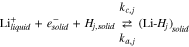
In the prior two publications associated with this work, major elements of the equation system to be described in this paper were used to examine a single-particle model of lithiated graphite along with Li plating and dissolution¹ and to examine the influence of inhomogeneities along the graphite surface in terms of promoting localized Li plating.² References 1 and 2 provide relevant literature reviews of models for Li plating as well. In this work, we extend the analyses to treat porous electrodes.

The first treatment of porous electrode models to consider Li plating during overcharge was provided by Arora, Doyle, and White.³ Several studies using variants of Ref. 3 have since appeared.^4–14 Quite recently, Lin¹⁵ employed a trained "long short-term memory (LSTM) neural network" to predict the anode electrode potential so as to avoid Li plating; Lin also provides a brief review of relevant Li plating literature. Campbell et al.¹³ detail the use of differential voltage spectroscopy for determining the onset of Li plating, which we also employ in this work (cf. Figs. 2 and 9). Campbell et al.¹³ also provide a thorough review of the experimental literature associated with the electrochemical detection of Li plating.

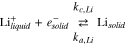
References 1 and 2 focused on two new additions to the literature. First, the treatment of possible exchange reactions between plated Li and galleries in the graphite host were introduced, (cf. the reaction rate (16) below and the corresponding resistance ${R}_{1-2}$ defined in Eq. 37). Second, previous studies of the lithium plating reaction^3–14 assumed that the activity coefficient of plated lithium was the same as that of bulk Li; when this assumption is used in a conventional charge-transfer relation (a Butler–Volmer equation), it yields the paradoxical result that the reverse of lithium plating (electro-dissolution) can occur, even when no plated lithium is present. The paradox was resolved by recognizing that small amounts of plated lithium (on the order of monolayers) interact with the graphite host, giving rise to an activity expression differing from that of bulk lithium, of the form in Eq. 9 below. In particular, the open-circuit voltage (OCV) of plated lithium becomes nonzero for these small amounts of plating, which prohibits complete depletion of the plated lithium in the Butler-Volmer equation.

The above modification to the activity of plated lithium comes at a price in complexity. The small surface coverage ${{\rm{\Gamma }}}_{ref}$ of plated lithium introduced in Eq. 9 dictates how large the surface coverage ${\rm{\Gamma }}$ must be, before its activity tends to that of bulk lithium, and ${{\rm{\Gamma }}}_{ref}$ is presumed to be on the order of monolayers. The resulting OCV ${U}_{2}$ of plated lithium thus becomes near singular, where it is essentially equal to zero until ${\rm{\Gamma }}$ decreases to approach ${{\rm{\Gamma }}}_{ref},$ at which point it rises rapidly for values of ${\rm{\Gamma }}\lt {{\rm{\Gamma }}}_{ref}.$ This near-singular behavior impacts solutions to the porous-electrode equations. In this work, we will consider lithiating a porous graphite electrode at constant current beyond the point at which plating starts to occur, followed by a period of open circuit, in which the plated lithium is re-absorbed into the graphite during equilibration. During constant lithiation, the plating first occurs on graphite particles at the electrode-separator interface. As the lithiation continues, the plating extends towards the copper current collector. This gives rise to two different regions of the electrode, separated by a moving boundary layer where, in the plated region, ${\rm{\Gamma }}\gg {{\rm{\Gamma }}}_{ref}$ and ${U}_{2}=0,$ whereas in the un-plated region ${\rm{\Gamma }}\ll {{\rm{\Gamma }}}_{ref}$ and ${U}_{2}\gt 0.$ The boundary layer is the thin region of the electrode where ${\rm{\Gamma }}$ and ${{\rm{\Gamma }}}_{ref}$ are approximately the same size. It is thus natural to consider solutions to the porous-electrode equations in the limiting case, for values of ${{\rm{\Gamma }}}_{ref}$ tending to zero.

The next section describes the porous-electrode equations and gives them in a dimensionless form. The dimensionless surface coverage $\bar{{\rm{\Gamma }}}$ (see Eq. 38) is the ratio of the amount of plating covering a spherical graphite particle of radius $a$ divided by the lithium capacity of the same particle at full intercalation. For a spherical particle of 5 micron radius, ${\bar{{\rm{\Gamma }}}}_{ref}={10}^{-3},$ which corresponds to 0.1 percent of the graphite capacity and about 2 monolayers of Li coverage. A set of equations is then derived for solutions to the limiting case, where ${\bar{{\rm{\Gamma }}}}_{ref}\,\to \,0.$ In the section on Simulation Results and Discussion, solutions to the equations will be shown for the value ${\bar{{\rm{\Gamma }}}}_{ref}={10}^{-3}.$ These solutions are compared to solutions of the limiting case, where ${\bar{{\rm{\Gamma }}}}_{ref}\,\to \,0.$ Finally, an Appendix describes some details of the numerical solution process.

Model Description

The porous electrode is modeled in a one-dimensional fashion using the coordinate $0\leqslant z\leqslant L,$ where the current collector is assumed to be at $z=0,$ and the separator interface is assumed to be at $z=L.$ For simplicity, we assume that the separator has zero thickness and the reference and counter electrode are placed at $z=L.$ At each point $z$ in the porous electrode, solid-phase diffusion occurs in a spherical graphite particle of radius $a,$ where both plating and lithium intercalation can occur at the interface between the electrolyte and the particle surface. As such, the geometric coordinates of this model correspond to $0\leqslant z\leqslant L,\,0\leqslant r\leqslant a.$ Figure 1 shows a schematic of the electrode and the coordinate system.

**Figure 1.** Schematic of the porous electrode. Dimensionless coordinates are $\bar{r}=r/a$ and $\bar{z}=z/L.$
Download figure:
Standard image High-resolution image

**Figure 1.** Schematic of the porous electrode. Dimensionless coordinates are $\bar{r}=r/a$ and $\bar{z}=z/L.$
Download figure:
Standard image High-resolution image

Thermodynamics and kinetics of the intercalation of lithium into graphite

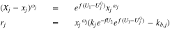
As was done in Refs. 1 and 2, the different galleries of intercalated lithium are assumed to be in thermodynamic equilibrium, so that their open-circuit potentials ${U}_{j}={U}_{1}$ for some common equilibrium potential ${U}_{1}$ of the graphite. A listing of parameters and properties can be found in Table I. The intercalation reaction in each gallery is represented as.

$\begin{eqnarray}&&{{\rm{Li}}}_{liquid}^{+}+{e}_{solid}^{-}+{H}_{j,solid}\,\begin{array}{c}{k}_{c,j}\\ \rightleftarrows \\ {k}_{a,j}\end{array}\,{\left(\mathrm{Li} \mbox{-} {H}_{j}\right)}_{solid}\end{eqnarray} \tag{ 1 }$

where ${H}_{j,solid}$ and ${\left(\mathrm{Li} \mbox{-} {H}_{j}\right)}_{solid}$ represent vacant and occupied sites for lithium in gallery j, ${{\rm{Li}}}_{liquid}^{+}$ is a lithium ion in the electrolyte and ${e}_{solid}^{-}$ is an electron in the graphite. For each gallery j

$\begin{eqnarray}&&{U}_{1}={U}_{j}^{0}+\displaystyle \frac{{\omega }_{j}}{f}\,\mathrm{ln}\left(\displaystyle \frac{{X}_{j}-{x}_{j}}{{x}_{j}}\right),\,f=\displaystyle \frac{F}{RT},\end{eqnarray} \tag{ 2 }$

$\begin{eqnarray}&&{x}_{j}=\frac{{X}_{j}}{1+\exp \left[f\left({U}_{1}-{U}_{j}^{0}\right)/{\omega }_{j}\right]},\,x\left({U}_{1}\right)=\sum {x}_{j}\end{eqnarray} \tag{ 3 }$

$\begin{eqnarray}&&\displaystyle \frac{dx}{d{U}_{1}}=-\displaystyle \sum _{j=1}^{N}\displaystyle \frac{f}{{\omega }_{j}}\displaystyle \frac{{X}_{j}\exp \left[f\left({U}_{1}-{U}_{j}^{0}\right)/{\omega }_{j}\right]}{{\left(1+\exp \left[f\left({U}_{1}-{U}_{j}^{0}\right)/{\omega }_{j}\right]\right)}^{2}}\end{eqnarray} \tag{ 4 }$

$\begin{eqnarray}&&{i}_{s,j}={i}_{0,j}\left[{e}^{\left(1-{\beta }_{j}\right)f{\eta }_{s,1}}-{e}^{-{\beta }_{j}f{\eta }_{s,1}}\right],\,{j}_{1}=\sum {i}_{s,j}\end{eqnarray} \tag{ 5 }$

$\begin{eqnarray}&&\begin{array}{l}{\eta }_{s,1}={{\rm{\Phi }}}_{1}-{{\rm{\Phi }}}_{2}-{U}_{1}\left(x\right)\,{\rm{and}}\\ {i}_{0,j}=\,{i}_{0,j}^{ref}{\left({x}_{j}\right)}^{{\omega }_{j}{\beta }_{j}}{\left({X}_{j}-{x}_{j}\right)}^{{\omega }_{j}\left(1-{\beta }_{j}\right)}{\left(\displaystyle \frac{{c}_{2}}{{c}_{0}}\right)}^{1-{\beta }_{j}}\end{array}\end{eqnarray} \tag{ 6 }$

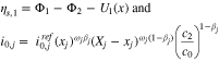
${{\rm{\Phi }}}_{1}$ is the solid-phase potential of the graphite, ${{\rm{\Phi }}}_{2}$ is the potential of the adjacent electrolyte, both with respect to the lithium reference electrode, and ${c}_{2}$ is the salt concentration in the electrolyte. Equation 6 can become singular when ${\omega }_{j}$ is close to zero and ${X}_{j}-{x}_{j}$ tends to zero as well. To avoid this, we rewrite Eq. 6 using

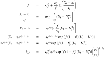
$\begin{eqnarray*}\begin{array}{rll}{U}_{1} & = & {U}_{j}^{0}+\displaystyle \frac{{\omega }_{j}}{f}\,\mathrm{ln}\left(\displaystyle \frac{{X}_{j}-{x}_{j}}{{x}_{j}}\right)\\ \displaystyle \frac{{X}_{j}-{x}_{j}}{{x}_{j}} & = & \exp \left[\displaystyle \frac{f}{{\omega }_{j}}\left({U}_{1}-{U}_{j}^{0}\right)\right]\\ {X}_{j}-{x}_{j} & = & {x}_{j}\exp \left[\displaystyle \frac{f}{{\omega }_{j}}\left({U}_{1}-{U}_{j}^{0}\right)\right]\\ {\left({X}_{j}-{x}_{j}\right)}^{{\omega }_{j}\left(1-{\beta }_{j}\right)} & = & {{x}_{j}}^{{\omega }_{j}\left(1-{\beta }_{j}\right)}\exp \left[f\left(1-{\beta }_{j}\right)\left({U}_{1}-{U}_{j}^{0}\right)\right]\\ {{x}_{j}}^{{\omega }_{j}{\beta }_{j}}{\left({X}_{j}-{x}_{j}\right)}^{{\omega }_{j}\left(1-{\beta }_{j}\right)} & = & {{x}_{j}}^{{\omega }_{j}}\exp \left[f\left(1-{\beta }_{j}\right)\left({U}_{1}-{U}_{j}^{0}\right)\right]\\ {i}_{0,j} & = & {i}_{0,j}^{ref}{{x}_{j}}^{{\omega }_{j}}\exp \left[f\left(1-{\beta }_{j}\right)\left({U}_{1}-{U}_{j}^{0}\right)\right]{\left(\displaystyle \frac{{c}_{2}}{{c}_{0}}\right)}^{1-{\beta }_{j}}\end{array}\end{eqnarray*}$

Table I. Parameters and properties.

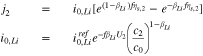
L, m	1.20E-04		${C}_{rate}$		1
a, m	5.00E-06		$I,$ A m⁻²		${C}_{rate}\tfrac{L{\varepsilon }_{1}{c}_{T}F}{3600\,{\rm{s}}}=73.454$
T, K	298		${{\rm{\Gamma }}}_{ref},$ mol m⁻²		$0.001{c}_{T}a/3=5.0753\,\times \,{10}^{-5}$
${c}_{0},$ mol m⁻³	1000		${U}_{1}\left(t=0\right),$ V		0.6
${i}_{0,Li}^{ref},$ A m⁻²	1		${t}_{+}^{0}$		0.4
${\beta }_{Li}$	0.5		${D}_{1},$ m² s⁻¹		$2\,\times \,{10}^{-14}$
${\beta }_{j}$	0.5		${i}_{0,j}^{ref},$ A m⁻²		1
${c}_{T},$ mol m⁻³	30452		$\gamma$		0.016757
${\varepsilon }_{2}$	0.25		${t}_{0},$ s		1250
${\tau }_{2}$	$1.8{\varepsilon }_{2}^{-0.53}$		Capacity, C m⁻²		$2.6444\,\times \,{10}^{5}$
${a}_{s}$	$3{\varepsilon }_{1}/a$		${R}_{e},$ Ohm-m²		$1.8014\,\times \,{10}^{-3}$
$\kappa ({c}_{0}),$ S m⁻¹	1		${R}_{s},$ Ohm-m²		$6.7087\,\times \,{10}^{-6}$
${D}_{2}\left({c}_{0}\right),$ m² s⁻¹	$2.58\,\times \,{10}^{-9}$		${R}_{d},$ Ohm-m²		$4.0463\,\times \,{10}^{-5}$
${\sigma }_{1},$ S m⁻¹	50		${R}_{k},$ Ohm-m²		$4.7555\,\times \,{10}^{-4}$
${\varepsilon }_{1}$	$1-{\varepsilon }_{2}$		${R}_{e,diff},$ Ohm-m²		$1.8583\,\times \,{10}^{-4}$
${\tau }_{1}$	$1.8{\varepsilon }_{1}^{-0.53}$


j=	1	2	3	4	5	6	7
${X}_{j}$	0.41336	0.23963	0.15018	0.05462	0.06744	0.05476	0.02
${U}_{j}^{0}$ (V)	0.08843	0.12799	0.14331	0.16984	0.21446	0.36325	0.088427
${\omega }_{j}$	0.08611	0.08009	0.72469	2.53277	0.09470	5.97354	1

We assume that all ${\beta }_{j}$ are equal, so one obtains from (5)

$\begin{eqnarray}&&{j}_{1}={i}_{0}\left[{e}^{\left(1-{\beta }_{j}\right)f{\eta }_{s}}-{e}^{-{\beta }_{j}f{\eta }_{s}}\right],\,{i}_{0}=\displaystyle \displaystyle \sum _{j}{i}_{0,j}\end{eqnarray} \tag{ 7 }$

Note that the same problem can in principle arise when ${x}_{j}$ becomes small, but this is less likely, as long as we stay away from zero intercalation. If it does occur, then one would have to use a special approximation for ${x}_{j}$ in the limit as it becomes small:

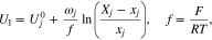
$\begin{eqnarray*}\begin{array}{lll}{x}_{j} & = & \displaystyle \frac{{X}_{j}}{1+\exp \left[f\left({U}_{1}-{U}_{j}^{0}\right)/{\omega }_{j}\right]}\approx \displaystyle \frac{{X}_{j}}{\exp \left[f\left({U}_{1}-{U}_{j}^{0}\right)/{\omega }_{j}\right]}\\ {{x}_{j}}^{{\omega }_{j}} & \approx & \displaystyle \frac{{X}_{j}^{{\omega }_{j}}}{\exp \left[f\left({U}_{1}-{U}_{j}^{0}\right)\right]}\end{array}\end{eqnarray*}$

Thermodynamics and kinetics of the lithium plating reaction

Lithium in the electrolyte can either intercalate into the graphite or plate on the graphite surface. The plating reaction is represented as

$\begin{eqnarray}&&{{\rm{Li}}}_{liquid}^{+}+{e}_{solid}^{-}\,\begin{array}{c}{k}_{c,Li}\\ \rightleftarrows \\ {k}_{a,Li}\end{array}\,{{\rm{Li}}}_{solid}\end{eqnarray} \tag{ 8 }$

The plated lithium is assumed to consist of a film of negligible thickness on the surface of the graphite particle, which can be characterized by a surface concentration ${\rm{\Gamma }}$ of plated lithium. Substantial lithium plating only occurs at cell potentials below zero with respect to a lithium reference, but sub-monolayer amounts of plated lithium are assumed to exist in an equilibrium state with intercalated lithium, even at higher cell potentials. As described in Refs. 1 and 2, we express the activity of Li as

$\begin{eqnarray}&&{a}_{Li}=1-\exp \left(-\displaystyle \frac{{\rm{\Gamma }}}{{{\rm{\Gamma }}}_{ref}}\right)=1-{e}^{-{\rm{\Theta }}},\,{\rm{\Theta }}=\displaystyle \frac{{\rm{\Gamma }}}{{{\rm{\Gamma }}}_{ref}}\end{eqnarray} \tag{ 9 }$

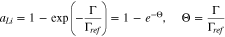
Thus, $\mathop{\mathrm{lim}}\limits_{{\rm{\Theta }}\to 0}{a}_{Li}={\rm{\Theta }}$ corresponds to the dilute-lithium, ideal-solution condition, and for ${\rm{\Theta }}\gg 1,$ ${a}_{Li}\,\to \,1,$ i.e., as the lithium surface concentration Γ grows larger than the reference value Γ_ref, the activity of the deposited Li rapidly (exponentially) approaches unity, which is the activity of bulk Li. The value of Γ_ref must be specified. For reasons outlined in Refs. 1 and 2, where the term relevant surface activity thickness is employed, we would expect Γ_ref to be a couple of monolayers of Li; for deposits of Li greater than this, we would expect the deposited Li to have the activity of bulk Li. The open-circuit potential ${U}_{2}$ for plated lithium can now be expressed as

$\begin{eqnarray}&&{U}_{2}=-\displaystyle \frac{1}{f}\,\mathrm{ln}\,{a}_{Li}=-\displaystyle \frac{1}{f}\,\mathrm{ln}\left(1-{e}^{-{\rm{\Theta }}}\right)=-\displaystyle \frac{{\mu }_{2}}{F}\end{eqnarray} \tag{ 10 }$

The chemical potential ${\mu }_{2}$ is relative to lithium metal. Large surface coverages of plated lithium, corresponding to values ${\rm{\Theta }}\gg 1,$ have the same potential as lithium metal, and ${U}_{2}$ tends to zero in this limit, but surface coverages less than ${{\rm{\Gamma }}}_{ref}$ develop positive potentials due to interactions with the graphite substrate. Based on formula 10, ${{\rm{\Gamma }}}_{ref}$ can be roughly viewed as the coverage at which lithium plating starts to occur. For example, when the plated lithium is equilibrated with intercalated lithium, ${U}_{1}={U}_{2};$ thus, at an equilibrium voltage of 1 mV and room temperature, the surface coverage is about $0.96\,{{\rm{\Gamma }}}_{ref},$ whereas at 1 V, the surface coverage drops to about ${10}^{-17}\,{{\rm{\Gamma }}}_{ref}.$

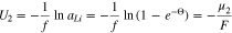
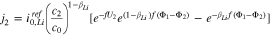
The kinetics of the lithium plating are given as

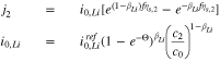
$\begin{eqnarray}\begin{array}{lll}{j}_{2} & = & {i}_{0,Li}\left[{e}^{\left(1-{\beta }_{Li}\right)f{\eta }_{s,2}}-{e}^{-{\beta }_{Li}f{\eta }_{s,2}}\right]\\ {i}_{0,Li} & = & {i}_{0,Li}^{ref}{\left(1-{e}^{-{\rm{\Theta }}}\right)}^{{\beta }_{Li}}{\left(\displaystyle \frac{{c}_{2}}{{c}_{0}}\right)}^{1-{\beta }_{Li}}\end{array}\end{eqnarray} \tag{ 11 }$

where ${\eta }_{s,2}={{\rm{\Phi }}}_{1}-{{\rm{\Phi }}}_{2}-{U}_{2}.$

If we use Eq. 10 to replace ${\rm{\Theta }}$ with ${U}_{2}$ in Eq. 11, we get

$\begin{eqnarray*}\begin{array}{lll}{j}_{2} & = & {i}_{0,Li}\left[{e}^{\left(1-{\beta }_{Li}\right)f{\eta }_{s,2}}-{e}^{-{\beta }_{Li}f{\eta }_{s,2}}\right]\\ {i}_{0,Li} & = & {i}_{0,Li}^{ref}{e}^{-f{\beta }_{Li}{U}_{2}}{\left(\displaystyle \frac{{c}_{2}}{{c}_{0}}\right)}^{1-{\beta }_{Li}}\end{array}\end{eqnarray*}$

$\begin{eqnarray}&&{j}_{2}={i}_{0,Li}^{ref}{\left(\displaystyle \frac{{c}_{2}}{{c}_{0}}\right)}^{1-{\beta }_{Li}}\left[{e}^{-f{U}_{2}}{e}^{\left(1-{\beta }_{Li}\right)f\left({{\rm{\Phi }}}_{1}-{{\rm{\Phi }}}_{2}\right)}-{e}^{-{\beta }_{Li}f\left({{\rm{\Phi }}}_{1}-{{\rm{\Phi }}}_{2}\right)}\right]\end{eqnarray} \tag{ 12 }$

We turn now to the case when a third reaction is occurring between the plated and graphite phases. At the interface between the lithiated graphite and the Li plating,

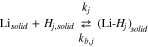
$\begin{eqnarray}&&{{\rm{Li}}}_{solid}+{H}_{j,solid}\,\begin{array}{c}{k}_{j}\\ \rightleftarrows \\ {k}_{b,j}\end{array}\,{\left(\mathrm{Li} \mbox{-} {H}_{j}\right)}_{solid}\end{eqnarray} \tag{ 13 }$

consistent with an elementary reaction when a Li deposit $\left({{\rm{Li}}}_{solid}\right)$ is on top of the lithiated graphite:

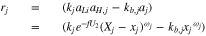
$\begin{eqnarray}\begin{array}{lll}{r}_{j} & = & \left({k}_{j}{a}_{Li}{a}_{H,j}-{k}_{b,j}{a}_{j}\right)\\ & = & \left({k}_{j}{e}^{-f{U}_{2}}{\left({X}_{j}-{x}_{j}\right)}^{{\omega }_{j}}-{k}_{b,j}{{x}_{j}}^{{\omega }_{j}}\right)\end{array}\end{eqnarray} \tag{ 14 }$

where there is one such reaction for each gallery. The activities are given as ${a}_{H,j}={\left({X}_{j}-{x}_{j}\right)}^{{\omega }_{j}}$ and ${a}_{j}={{x}_{j}}^{{\omega }_{j}}$ for vacant and occupied sites in gallery j. From Eq. 2,

$\begin{eqnarray*}\begin{array}{lll}{\left({X}_{j}-{x}_{j}\right)}^{{\omega }_{j}} & = & {e}^{f\left({U}_{1}-{U}_{j}^{0}\right)}{{x}_{j}}^{{\omega }_{j}}\\ {r}_{j} & = & {{x}_{j}}^{{\omega }_{j}}\left({k}_{j}{e}^{-f{U}_{2}}{e}^{f\left({U}_{1}-{U}_{j}^{0}\right)}-{k}_{b,j}\right)\end{array}\end{eqnarray*}$

Note that at equilibrium, ${U}_{1}={U}_{2},$ so that

$\begin{eqnarray*}&&\displaystyle \frac{{k}_{j}}{{k}_{b,j}}={e}^{f{U}_{j}^{0}}\end{eqnarray*}$

$\begin{eqnarray*}&&{r}_{j}={k}_{b,j}{{x}_{j}}^{{\omega }_{j}}\left({e}^{f\left({U}_{1}-{U}_{2}\right)}-1\right)\end{eqnarray*}$

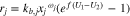
Summing all reactions together, one gets

$\begin{eqnarray}&&{r}_{T}=\displaystyle \displaystyle \sum _{j}{r}_{j}=\left(\displaystyle \displaystyle \sum _{j}{k}_{b,j}{{x}_{j}}^{{\omega }_{j}}\right)\left({e}^{f\left({U}_{1}-{U}_{2}\right)}-1\right)\end{eqnarray} \tag{ 15 }$

In what follows, for simplicity it is assumed that all ${k}_{b,j}=k,$ so that

$\begin{eqnarray}&&{r}_{T}=k\left(\displaystyle \displaystyle \sum _{j}{{x}_{j}}^{{\omega }_{j}}\right)\left({e}^{f\left({U}_{1}-{U}_{2}\right)}-1\right)\end{eqnarray} \tag{ 16 }$

The relevant thermodynamics for the problem formulation are depicted in Fig. 2, where the abscissa $\bar{Q}$ refers to

$\begin{eqnarray}&&\bar{Q}=\displaystyle \frac{Q}{F{c}_{T}{\varepsilon }_{1}}\end{eqnarray} \tag{ 17 }$

where $Q$ is the total charge (e.g., units of C cm⁻³) of plated and intercalated lithium. At equilibrium, ${U}_{1}={U}_{2}=U.$ For ${\bar{{\rm{\Gamma }}}}_{ref}$ below 0.001, which (for a particle radius of 5 micron) corresponds to the reference surface coverage of Li being 0.1 percent of the specific areal capacity for deposited Li, further reductions in ${\bar{{\rm{\Gamma }}}}_{ref}$ do not influence significantly the equilibrium results as plotted. The lower plot in Fig. 2 portrays the highly nonlinear behavior in $\tfrac{dU}{d\bar{Q}}$ and the dimensionless effective diffusion coefficient, relevant to the diffusion of lithium in the graphite discussed below, $-fx\left(1-x\right)\tfrac{d{U}_{1}}{dx}.$ In addition, we see that differentiation of the OCV curve ( $\partial U/\partial \bar{Q}\,{\rm{vs}}\,\bar{Q}$ ) yields a sharp valley (a pronounced minimum) as (i) the graphite fills with Li and $x\,\to \,1,$ leading to a sharp decline in the potential and $\partial U/\partial \bar{Q},$ followed by (ii) Li plating, causing $U\,\to \,0\,\,V,$ a constant, and causing $\partial U/\partial \bar{Q}$ to transition from a large, negative value to nearly zero. These observations underscore the relevance of evaluating $\partial U/\partial \bar{Q}$ to approximate the onset of Li plating (cf. Fig. 9).

**Figure 2.** Equilibrium potential (upper plot) and, in the lower plots, its differential vs dimensionless charge and the dimensionless, effective diffusion coefficient vs the fraction of Li-filled sites.
Download figure:
Standard image High-resolution image

Charge and material transport in a porous electrode

Plated lithium covers the surface of each graphite particle and a mass balance for this surface coverage implies that at $r=a$

$\begin{eqnarray}&&F{{\rm{\Gamma }}}_{ref}\displaystyle \frac{\partial {\rm{\Theta }}}{\partial t}=-{j}_{2}-F{r}_{T}\end{eqnarray} \tag{ 18 }$

that is, the rate of growth of the surface coverage is the difference between the rate at which lithium is plated and the rate at which it transports into the graphite under reaction 13.

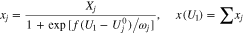
Diffusive transport of intercalated lithium in a spherical graphite particle is given as (Refs. 1 and 2)

$\begin{eqnarray}&&{c}_{T}\displaystyle \frac{\partial x}{\partial t}=-\displaystyle \frac{{c}_{T}}{{r}^{2}}\displaystyle \frac{\partial }{\partial r}\left({r}^{2}x\left(1-x\right)f{D}_{1}\displaystyle \frac{d{U}_{1}}{dx}\displaystyle \frac{\partial x}{\partial r}\right)\end{eqnarray} \tag{ 19 }$

where $x$ is the mole fraction of occupied lithium sites, $D$ is a solid phase diffusion coefficient, and ${c}_{T}$ is the total concentration of sites (occupied and unoccupied) in the graphite. Because the relation $x\left({U}_{1}\right)$ is given explicitly in Eq. 3, whereas the relationship ${U}_{1}\left(x\right)$ must be numerically inverted, it is convenient to reformulate Eq. 19 in terms of the dependent variable ${U}_{1}:$

$\begin{eqnarray}&&\displaystyle \frac{\partial x}{\partial {U}_{1}}\displaystyle \frac{\partial {U}_{1}}{\partial t}=-\displaystyle \frac{1}{{r}^{2}}\displaystyle \frac{\partial }{\partial r}\left({r}^{2}x\left(1-x\right)f{D}_{1}\displaystyle \frac{\partial {U}_{1}}{\partial r}\right)\end{eqnarray} \tag{ 20 }$

where $\partial x/\partial {U}_{1}$ is given by Eq. 4. The boundary condition at the particle surface $r=a$ is given as

$\begin{eqnarray}&&F{c}_{T}{D}_{1}x\left(1-x\right)f{\left.\displaystyle \frac{\partial {U}_{1}}{\partial r}\right|}_{r=a}={j}_{1}-F{r}_{T}\end{eqnarray} \tag{ 21 }$

Of particular interest is the case when the reaction rate ${r}_{T}$ is infinitely fast, that is, $k=\infty .$ In this case Eqs. 18 and 21 collapse and become redundant. The problem can be corrected replacing Eq. 18 by the difference of Eqs. 18 and 21:

$\begin{eqnarray}&&F{{\rm{\Gamma }}}_{ref}\displaystyle \frac{\partial {\rm{\Theta }}}{\partial t}=-{j}_{1}-{j}_{2}+F{c}_{T}{D}_{1}x\left(1-x\right)f{\left.\displaystyle \frac{\partial {U}_{1}}{\partial r}\right|}_{r=a}\end{eqnarray} \tag{ 22 }$

The boundary condition (21) continues to be valid, but in the limit $k\,\to \,\infty ,$ it reduces to the equilibrium condition

$\begin{eqnarray}&&{U}_{1}={U}_{2}\end{eqnarray} \tag{ 23 }$

at $r=a.$

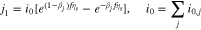
Just as there is a choice between the variables $x$ and ${U}_{1}$ in the graphite, there is also a choice between the variables ${\rm{\Theta }}$ and ${U}_{2}$ in Eq. 22, where the transformation (10) relates the two variables. Unfortunately, neither of these choices is optimal for numerical calculations. When starting to charge an empty cell, the variable ${\rm{\Theta }}$ is very small, and caution must be taken to prohibit it from going negative during numerical iterations. It also becomes difficult to determine ${\rm{\Theta }}$ with enough accuracy to accurately determine ${U}_{2}$ via Eq. 10. Similarly, when plating occurs, the variable ${U}_{2}$ tends to zero and the amount of accuracy needed to back-calculate ${\rm{\Theta }}$ using Eq. 10 becomes prohibitive. 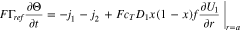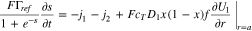In summary, it is desirable to use ${U}_{2}$ as the dependent variable during charging, but ${\rm{\Theta }}$ is the preferred choice when plating has occurred. There is a third alternative that contains the best of both choices, but it entails defining a new dependent variable, which we refer to as $s.$ ^1,2 We define s by requiring it to satisfy the differential equation

$\begin{eqnarray}&&ds=d{\rm{\Theta }}-fd{U}_{2}\end{eqnarray} \tag{ 24 }$

The idea behind Eq. 24 is that at small states of charge, $d{\rm{\Theta }}$ will be negligible so that s will be proportional to $-f{U}_{2},$ whereas when plating has occurred, $fd{U}_{2}$ will be negligible and $s$ will be proportional to ${\rm{\Theta }}.$ The different signs for $d{\rm{\Theta }}$ and $fd{U}_{2}$ in Eq. 24 arise because the variable ${\rm{\Theta }}$ increases as $f{U}_{2}$ decreases. Eq. 24 can be solved as follows:

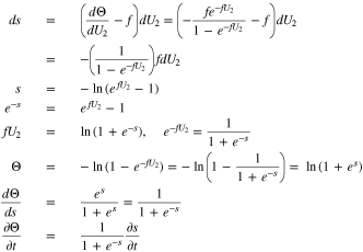
$\begin{eqnarray}\begin{array}{rll}ds & = & \left(\displaystyle \frac{d{\rm{\Theta }}}{d{U}_{2}}-f\right)d{U}_{2}=\left(-\displaystyle \frac{f{e}^{-f{U}_{2}}}{1-{e}^{-f{U}_{2}}}-f\right)d{U}_{2}\\ & = & -\left(\displaystyle \frac{1}{1-{e}^{-f{U}_{2}}}\right)fd{U}_{2}\\ s & = & -\,\mathrm{ln}\left({e}^{f{U}_{2}}-1\right)\\ {e}^{-s} & = & {e}^{f{U}_{2}}-1\\ f{U}_{2} & = & \mathrm{ln}\left(1+{e}^{-s}\right),\,{e}^{-f{U}_{2}}=\displaystyle \frac{1}{1+{e}^{-s}}\\ {\rm{\Theta }} & = & -\,\mathrm{ln}\left(1-{e}^{-f{U}_{2}}\right)=-\,\mathrm{ln}\left(1-\displaystyle \frac{1}{1+{e}^{-s}}\right)=\,\mathrm{ln}\left(1+{e}^{s}\right)\\ \displaystyle \frac{d{\rm{\Theta }}}{ds} & = & \displaystyle \frac{{e}^{s}}{1+{e}^{s}}=\displaystyle \frac{1}{1+{e}^{-s}}\\ \displaystyle \frac{\partial {\rm{\Theta }}}{\partial t} & = & \displaystyle \frac{1}{1+{e}^{-s}}\displaystyle \frac{\partial s}{\partial t}\end{array}\end{eqnarray} \tag{ 25 }$

With these conventions, Eq. 22 becomes

$\begin{eqnarray}&&\displaystyle \frac{F{{\rm{\Gamma }}}_{ref}}{1+{e}^{-s}}\displaystyle \frac{\partial s}{\partial t}=-{j}_{1}-{j}_{2}+F{c}_{T}{D}_{1}x\left(1-x\right)f{\left.\displaystyle \frac{\partial {U}_{1}}{\partial r}\right|}_{r=a}\end{eqnarray} \tag{ 26 }$

Equation 26, along with

$\begin{eqnarray}&&{\rm{\Theta }}=\,\mathrm{ln}\left(1+{e}^{s}\right),\,{U}_{2}=\displaystyle \frac{1}{f}\,\mathrm{ln}\left(1+{e}^{-s}\right)\end{eqnarray} \tag{ 27 }$

replace Eq. 22. In the limit of large k, when reaction 13 becomes facile, Eq. 21 becomes

$\begin{eqnarray}&&{U}_{1}={U}_{2}\left(s\right)\end{eqnarray} \tag{ 28 }$

at $r=a.$

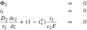
The transport equations in the electrolyte of the porous electrode are well known¹ and take the form

$\begin{eqnarray}&&\displaystyle \frac{\partial {i}_{2}}{\partial z}={a}_{s}\left({j}_{1}+{j}_{2}\right)\end{eqnarray} \tag{ 29 }$

$\begin{eqnarray}&&{i}_{2}=\displaystyle \frac{{\varepsilon }_{2}}{{\tau }_{2}}{\kappa }_{2}\left(-\displaystyle \frac{\partial {{\rm{\Phi }}}_{2}}{\partial z}+\displaystyle \frac{2RT}{F}\left(1+\displaystyle \frac{d\,\mathrm{ln}\,{f}_{\pm }}{d\,\mathrm{ln}\,{c}_{2}}\right)\left(1-{t}_{+}^{0}\right)\displaystyle \frac{\partial }{\partial z}\,\mathrm{ln}\left({c}_{2}\right)\right)\end{eqnarray} \tag{ 30 }$

$\begin{eqnarray}&&{i}_{1}=-\displaystyle \frac{{\varepsilon }_{1}}{{\tau }_{1}}\sigma \displaystyle \frac{\partial {{\rm{\Phi }}}_{1}}{\partial z}\end{eqnarray} \tag{ 31 }$

$\begin{eqnarray}&&\displaystyle \frac{\partial {i}_{1}}{\partial z}=-{a}_{s}\left({j}_{1}+{j}_{2}\right)\end{eqnarray} \tag{ 32 }$

$\begin{eqnarray}&&\displaystyle \frac{\partial {c}_{2}}{\partial t}=\displaystyle \frac{\partial }{\partial z}\left(\displaystyle \frac{{D}_{2}}{{\tau }_{2}}\displaystyle \frac{\partial {c}_{2}}{\partial z}+\left(1-{t}_{+}^{0}\right)\displaystyle \frac{{i}_{2}}{{\varepsilon }_{2}F}\right)\end{eqnarray} \tag{ 33 }$

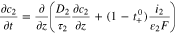
For charging at a constant current density $I,$ boundary conditions at the current collector $z=0$ are

$\begin{eqnarray}\begin{array}{lll}{i}_{1} & = & I\\ {i}_{2} & = & 0\\ \displaystyle \frac{{D}_{2}}{{\tau }_{2}}\displaystyle \frac{\partial {c}_{2}}{\partial z} & = & 0\end{array}\end{eqnarray} \tag{ 34 }$

At the separator interface $z=L,$ the location of the reference electrode,

$\begin{eqnarray}\begin{array}{lll}{{\rm{\Phi }}}_{2} & = & 0\\ {i}_{1} & = & 0\\ \displaystyle \frac{{D}_{2}}{{\tau }_{2}}\displaystyle \frac{\partial {c}_{2}}{\partial z}+\left(1-{t}_{+}^{0}\right)\displaystyle \frac{{i}_{2}}{{\varepsilon }_{2}F} & = & 0\end{array}\end{eqnarray} \tag{ 35 }$

At the start of charging, we assume that all the graphite is at some high OCV, in our case,

$\begin{eqnarray}&&\begin{array}{l}{U}_{1}=0.6{\rm{V}}={U}_{2}\\ {c}_{2}={c}_{0}\end{array}\end{eqnarray} \tag{ 36 }$

where ${c}_{0}$ is the bulk value of salt concentration in the electrolyte.

Dimensionless equations

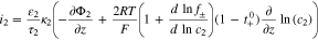
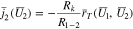
We define the following resistances

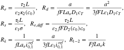
$\begin{eqnarray}&&\begin{array}{l}{R}_{e}=\displaystyle \frac{{\tau }_{2}L}{{\varepsilon }_{2}{\kappa }_{2}\left({c}_{0}\right)},\,{R}_{d}=\displaystyle \frac{a}{fFL{a}_{s}{D}_{1}{c}_{T}}=\displaystyle \frac{{a}^{2}}{3fFL{\varepsilon }_{1}{D}_{1}{c}_{T}},\\ {R}_{s}=\displaystyle \frac{{\tau }_{1}L}{{\varepsilon }_{1}\sigma },\,{R}_{e,diff}=\displaystyle \frac{{\tau }_{2}L}{{\varepsilon }_{2}fF{D}_{2}\left({c}_{0}\right){c}_{0}},\\ {R}_{k}=\displaystyle \frac{1}{fL{a}_{s}{i}_{0,1}^{ref}}=\displaystyle \frac{a}{3fL{\varepsilon }_{1}{i}_{0,1}^{ref}},\,{R}_{1-2}=\displaystyle \frac{1}{FfL{a}_{s}k}\end{array}\end{eqnarray} \tag{ 37 }$

where one can view ${R}_{e}$ as a characteristic electrolyte resistance, ${R}_{d}$ as a solid-phase diffusion resistance, ${R}_{s}$ as a solid phase electron resistance, ${R}_{e,diff}$ as a salt diffusion resistance, ${R}_{k}$ as a charge transfer resistance for intercalation and ${R}_{1-2}$ as the resistance associated to the interface reaction between the plated and graphite phases. Additionally, define

$\begin{eqnarray}&&\begin{array}{l}{c}_{2}={c}_{0}{\bar{c}}_{2},\,{\bar{D}}_{2}=\displaystyle \frac{{D}_{2}({c}_{2})}{{D}_{2}\left({c}_{0}\right)},\,\bar{\kappa }=\displaystyle \frac{\kappa ({c}_{2})}{\kappa \left({c}_{0}\right)},\,{j}_{1}={i}_{0,1}^{ref}{\bar{j}}_{1},\\ {j}_{2}={i}_{0,1}^{ref}{\bar{j}}_{2},\,{r}_{T}=k{\bar{r}}_{T},\,z=L\bar{z},\,r=a\bar{r},\,{t}_{0}=\displaystyle \frac{{a}^{2}}{{D}_{1}},\,\tau =\displaystyle \frac{t}{{t}_{0}},\\ \gamma =\displaystyle \frac{{\tau }_{2}{L}^{2}}{{D}_{2}\left({c}_{0}\right){t}_{0}},\,{i}_{0,Li}^{ref}={i}_{0,1}^{ref}{\bar{i}}_{0,Li}^{ref},\,{i}_{2}=\displaystyle \frac{1}{f{R}_{e}}{\bar{i}}_{2},\,{i}_{1}=\displaystyle \frac{1}{f{R}_{s}}{\bar{i}}_{1},\\ {{\rm{\Phi }}}_{k}=\displaystyle \frac{{\bar{{\rm{\Phi }}}}_{k}}{f},\,{U}_{i}=\displaystyle \frac{{\bar{U}}_{i}}{f},\,\bar{{\rm{\Gamma }}}=\displaystyle \frac{3{\rm{\Gamma }}}{a{c}_{T}},\,{\bar{{\rm{\Gamma }}}}_{ref}=\displaystyle \frac{3{{\rm{\Gamma }}}_{ref}}{a{c}_{T}}\\ I=\displaystyle \frac{\bar{I}}{f{R}_{s}}\end{array}\end{eqnarray} \tag{ 38 }$

In dimensionless form, the electrode is in the region $0\leqslant \bar{z}\leqslant 1$ with the separator at $\bar{z}=1$ and the current collector at $\bar{z}=0$ (cf. Fig. 1). The solid phase diffusion equation becomes

$\begin{eqnarray}&&\displaystyle \frac{dx}{d{\bar{U}}_{1}}\displaystyle \frac{\partial {\bar{U}}_{1}}{\partial \tau }=-\displaystyle \frac{1}{{\bar{r}}^{2}}\displaystyle \frac{\partial }{\partial \bar{r}}\left({\bar{r}}^{2}x\left(1-x\right)\displaystyle \frac{\partial {\bar{U}}_{1}}{\partial \bar{r}}\right)\end{eqnarray} \tag{ 39 }$

and equations for the unknowns ${\bar{{\rm{\Phi }}}}_{1},{\bar{{\rm{\Phi }}}}_{2}$ and ${\bar{c}}_{2}$ take the form

$\begin{eqnarray}&&\displaystyle \frac{\partial {\bar{i}}_{2}}{\partial \bar{z}}=\displaystyle \frac{{R}_{e}}{{R}_{k}}\left({\bar{j}}_{1}+{\bar{j}}_{2}\right)\end{eqnarray} \tag{ 40 }$

$\begin{eqnarray}&&{\bar{i}}_{2}=\bar{\kappa }\left(-\displaystyle \frac{\partial {\bar{{\rm{\Phi }}}}_{2}}{\partial \bar{z}}+2\left(1+\displaystyle \frac{d\,\mathrm{ln}\,{f}_{\pm }}{d\,\mathrm{ln}\,{c}_{2}}\right)\left(1-{t}_{+}^{0}\right)\displaystyle \frac{\partial }{\partial \bar{z}}\,\mathrm{ln}\left({\bar{c}}_{2}\right)\right)\end{eqnarray} \tag{ 41 }$

$\begin{eqnarray}&&{\bar{i}}_{1}=-\displaystyle \frac{\partial {\bar{{\rm{\Phi }}}}_{1}}{\partial \bar{z}}\end{eqnarray} \tag{ 42 }$

$\begin{eqnarray}&&\displaystyle \frac{\partial {\bar{i}}_{1}}{\partial \bar{z}}=-\displaystyle \frac{{R}_{s}}{{R}_{k}}\left({\bar{j}}_{1}+{\bar{j}}_{2}\right)\end{eqnarray} \tag{ 43 }$

$\begin{eqnarray}&&\gamma \displaystyle \frac{\partial {\bar{c}}_{2}}{\partial \tau }=\displaystyle \frac{\partial }{\partial \bar{z}}\left({\bar{D}}_{2}\displaystyle \frac{\partial {\bar{c}}_{2}}{\partial \bar{z}}\right)+\displaystyle \frac{{R}_{e,diff}}{{R}_{k}}\left(1-{t}_{+}^{0}\right)\left({\bar{j}}_{1}+{\bar{j}}_{2}\right)\end{eqnarray} \tag{ 44 }$

The plating reaction takes the form (at $\bar{r}=1$ )

$\begin{eqnarray}\begin{array}{lll}\displaystyle \frac{1}{3}\displaystyle \frac{\partial \bar{{\rm{\Gamma }}}}{\partial \tau } & = & \displaystyle \frac{{\bar{{\rm{\Gamma }}}}_{ref}}{3}\displaystyle \frac{\partial {\rm{\Theta }}}{\partial \tau }=-\displaystyle \frac{{R}_{d}}{{R}_{k}}{\bar{j}}_{2}-\displaystyle \frac{{R}_{d}}{{R}_{1-2}}{\bar{r}}_{T}\\ & = & -\displaystyle \frac{{R}_{d}}{{R}_{k}}\left({\bar{j}}_{1}+{\bar{j}}_{2}\right)+x\left(1-x\right){\left.\displaystyle \frac{\partial {\bar{U}}_{1}}{\partial \bar{r}}\right|}_{\bar{r}=1}\end{array}\end{eqnarray} \tag{ 45 }$

$\begin{eqnarray}&&x\left(1-x\right){\left.\displaystyle \frac{\partial {\bar{U}}_{1}}{\partial \bar{r}}\right|}_{\bar{r}=1}=\displaystyle \frac{{R}_{d}}{{R}_{k}}{\bar{j}}_{1}-\displaystyle \frac{{R}_{d}}{{R}_{1-2}}{\bar{r}}_{T}\left({\bar{U}}_{1},{\bar{U}}_{2}\right)\end{eqnarray} \tag{ 46 }$

When ${R}_{1-2}=0,$ Eq. 46 is replaced with

$\begin{eqnarray}&&{\bar{U}}_{1}={\bar{U}}_{2}\end{eqnarray} \tag{ 47 }$

The dimensionless form of Eq. 26 becomes

$\begin{eqnarray}&&\displaystyle \frac{{\bar{{\rm{\Gamma }}}}_{ref}}{1+{e}^{-s}}\displaystyle \frac{\partial s}{\partial \tau }=-\displaystyle \frac{{R}_{d}}{{R}_{k}}\left({j}_{1}+{j}_{2}\right)+x\left(1-x\right){\left.\displaystyle \frac{\partial {U}_{1}}{\partial \bar{r}}\right|}_{\bar{r}=1}\end{eqnarray} \tag{ 48 }$

At the separator interface $\bar{z}=1,$

$\begin{eqnarray}\begin{array}{rll}{\bar{{\rm{\Phi }}}}_{2} & = & 0\\ \displaystyle \frac{\partial {\bar{{\rm{\Phi }}}}_{1}}{\partial \bar{z}} & = & 0\\ \left(1-{t}_{+}^{0}\right){\bar{i}}_{2} & = & -\displaystyle \frac{{R}_{e}}{{R}_{e,diff}}{\bar{D}}_{2}\displaystyle \frac{\partial {\bar{c}}_{2}}{\partial \bar{z}}\end{array}\end{eqnarray} \tag{ 49 }$

At the current collector $\bar{z}=0,$

$\begin{eqnarray}\begin{array}{rll}\displaystyle \frac{\partial {\bar{{\rm{\Phi }}}}_{2}}{\partial \bar{z}} & = & 0\\ \displaystyle \frac{\partial {\bar{c}}_{2}}{\partial \bar{z}} & = & 0\\ {\bar{i}}_{1} & = & \bar{I}\end{array}\end{eqnarray} \tag{ 50 }$

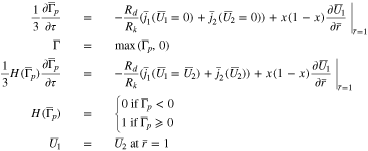
Equations in the limiting case ${\bar{{\rm{\Gamma }}}}_{ref}\,\to \,0$

In this limit, the variable ${\rm{\Theta }}$ must be abandoned, and it must be replaced with the variable $\bar{{\rm{\Gamma }}}.$ Note also from Eq. 10 that ${\rm{\Gamma }}=0$ for any finite positive value of ${U}_{2}$ in this limit. We must consider three different situations.

Case 1: No plating has occurred. In this case, $\bar{{\rm{\Gamma }}}=0$ and Eq. 45 at the particle surface $\bar{r}=1$ become

$\begin{eqnarray}\begin{array}{rll}\bar{{\rm{\Gamma }}} & = & 0\\ {\bar{j}}_{2}\left({\bar{U}}_{2}\right) & = & -\displaystyle \frac{{R}_{k}}{{R}_{1-2}}{\bar{r}}_{T}\left({\bar{U}}_{1},{\bar{U}}_{2}\right)\\ x\left(1-x\right){\left.\displaystyle \frac{\partial {\bar{U}}_{1}}{\partial \bar{r}}\right|}_{\bar{r}=1} & = & \displaystyle \frac{{R}_{d}}{{R}_{k}}\left({\bar{j}}_{1}+{\bar{j}}_{2}\right)\end{array}\end{eqnarray} \tag{ 51 }$

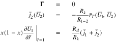
The second of Eq. 51 can be used to determine ${\bar{U}}_{2}$ as a function of ${\bar{U}}_{1}$ and the other dependent variables. During charging at constant current, one must monitor the potential ${\bar{U}}_{2}$ at the separator interface $\bar{z}=1$ continually while solving. Once ${\bar{U}}_{2}\left(\bar{z}=1\right)=0,$ plating will start and the equations in Case 2 must then be solved. When ${R}_{1-2}=0,$ the second of Eq. 51 becomes

$\begin{eqnarray}&&{\bar{r}}_{T}=0\,{\rm{or}}\,{\rm{equivalently}}\,{\bar{U}}_{2}={\bar{U}}_{1}\end{eqnarray} \tag{ 52 }$

This condition should be understood as describing the situation when the rate constant $k$ for the reactions 13 becomes infinite, and the plated and intercalated phases of lithium are always equilibrated.

Case 2: Plating occurs, and the region of plating is expanding in time from the separator interface at $\bar{z}=1$ toward the current collector at $\bar{z}=0.$ This situation holds once plating occurs during charging at a sufficiently large constant current $\bar{I}.$ In this case, one must introduce an additional variable ${\bar{U}}_{2,np}$ and Eqs. 45 and 46 become

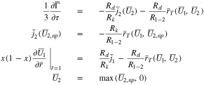
$\begin{eqnarray}\begin{array}{rll}\displaystyle \frac{1}{3}\displaystyle \frac{\partial \bar{{\rm{\Gamma }}}}{\partial \tau } & = & -\displaystyle \frac{{R}_{d}}{{R}_{k}}{\bar{j}}_{2}\left({\bar{U}}_{2}\right)-\displaystyle \frac{{R}_{d}}{{R}_{1-2}}{\bar{r}}_{T}\left({\bar{U}}_{1},{\bar{U}}_{2}\right)\\ {\bar{j}}_{2}\left({\bar{U}}_{2,np}\right) & = & -\displaystyle \frac{{R}_{k}}{{R}_{1-2}}{\bar{r}}_{T}\left({\bar{U}}_{1},{\bar{U}}_{2,np}\right)\\ x\left(1-x\right){\left.\displaystyle \frac{\partial {\bar{U}}_{1}}{\partial \bar{r}}\right|}_{\bar{r}=1} & = & \displaystyle \frac{{R}_{d}}{{R}_{k}}{\bar{j}}_{1}-\displaystyle \frac{{R}_{d}}{{R}_{1-2}}{\bar{r}}_{T}\left({\bar{U}}_{1},{\bar{U}}_{2}\right)\\ {\bar{U}}_{2} & = & \max \left({\bar{U}}_{2,np},0\right)\end{array}\end{eqnarray} \tag{ 53 }$

Note that only the second of the above equations depends on ${\bar{U}}_{2,np};$ the first and third equations are evaluated using ${\bar{U}}_{2}$ instead. In this way, the entire electrode is automatically divided into a region where no plating has occurred, and ${\bar{U}}_{2}={\bar{U}}_{2,np}\gt 0,$ and a region where plating is occurring, and ${\bar{U}}_{2}=0.$ After solving Eq. 53, the interface ${\bar{z}}_{0}$ between the plated and non-plated regions can be determined by using Newton iteration to find the zero of the function ${\bar{U}}_{2,np}\left(\bar{z}\right);$ however, this can be done as a post-processing step, and it is not necessary to determine ${\bar{z}}_{0}$ in order to solve Eq. 53. This is the advantage of the above formulation: It solves a single set of equations in both the plated and un-plated regions, so that it is not necessary to treat each region separately. Note in addition that, in the region where no plating has occurred, ${\bar{U}}_{2}={\bar{U}}_{2,np}\gt 0,$ so that the first and second of Eq. 53 imply that in this region $\partial \,\bar{{\rm{\Gamma }}}/\partial \tau =0$ and, assuming that $\bar{{\rm{\Gamma }}}=0$ is the initial condition, $\bar{{\rm{\Gamma }}}$ will remain zero in the un-plated region.

When ${R}_{1-2}=0,$ Eq. 53 must be modified to

$\begin{eqnarray}\begin{array}{rll}\displaystyle \frac{1}{3}\displaystyle \frac{\partial \bar{{\rm{\Gamma }}}}{\partial \tau } & = & -\displaystyle \frac{{R}_{d}}{{R}_{k}}\left({\bar{j}}_{1}\left({\bar{U}}_{1}={\bar{U}}_{2}\right)+{\bar{j}}_{2}\left({\bar{U}}_{2}\right)\right)+x\left(1-x\right){\left.\displaystyle \frac{\partial {\bar{U}}_{1}}{\partial \bar{r}}\right|}_{\bar{r}=1}\\ x\left(1-x\right){\left.\displaystyle \frac{\partial {\bar{U}}_{1}}{\partial \bar{r}}\right|}_{\bar{r}=1} & = & \displaystyle \frac{{R}_{d}}{{R}_{k}}\left({\bar{j}}_{1}\left({\bar{U}}_{1}={\bar{U}}_{2,np}\right)+{\bar{j}}_{2}\left({\bar{U}}_{2}={\bar{U}}_{2,np}\right)\right)\\ {\bar{U}}_{1} & = & {\bar{U}}_{2}\,{\rm{at}}\,\bar{r}=1\\ {\bar{U}}_{2} & = & \max \left({\bar{U}}_{2,np},0\right)\end{array}\end{eqnarray} \tag{ 54 }$

In this case, the flux condition (third of Eq. 53) becomes a Dirichlet condition (the third of Eq. 54), and the second equation, determining ${\bar{U}}_{2,np},$ now involves the flux at the particle surface. Eq. 53 assume that the function ${\bar{U}}_{2}\left(\bar{z}\right)$ is continuous at the interface ${\bar{z}}_{0}$ between the plated and un-plated regions so that, in particular, ${\bar{U}}_{2}\left({\bar{z}}_{0}\right)=0.$ As will be seen in Fig. 8, this assumption is not generally true when one switches from charging to open circuit (Case 3 below).

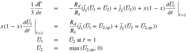
Case 3: Plating exists, but the region of plating is decreasing in size over time, for example, when the cell goes to open circuit after charging. In this case, we introduce two new variables: ${\bar{U}}_{2,np}$ and ${\bar{{\rm{\Gamma }}}}_{p}.$ Equations 45 and 46 become

$\begin{eqnarray}\begin{array}{rll}\displaystyle \frac{1}{3}\displaystyle \frac{\partial {\bar{{\rm{\Gamma }}}}_{p}}{\partial \tau } & = & -\displaystyle \frac{{R}_{d}}{{R}_{k}}{\bar{j}}_{2}\left({\bar{U}}_{2}=0\right)-\displaystyle \frac{{R}_{d}}{{R}_{1-2}}{\bar{r}}_{T}\left({\bar{U}}_{1},{\bar{U}}_{2}=0\right)\\ \bar{{\rm{\Gamma }}} & = & \max \left({\bar{{\rm{\Gamma }}}}_{p},0\right)\\ {\bar{j}}_{2}\left({\bar{U}}_{2,np}\right) & = & -\displaystyle \frac{{R}_{k}}{{R}_{1-2}}{\bar{r}}_{T}\left({\bar{U}}_{1},{\bar{U}}_{2,np}\right)\\ {\bar{U}}_{2} & = & H\left(-{\bar{{\rm{\Gamma }}}}_{p}\right){\bar{U}}_{2,np}\,H\left(-{\bar{{\rm{\Gamma }}}}_{p}\right)=\left\{\begin{array}{c}1\,{\rm{if}}\,{\bar{{\rm{\Gamma }}}}_{p}\leqslant 0\\ 0\,{\rm{if}}\,{\bar{{\rm{\Gamma }}}}_{p}\gt 0\end{array}\right.\\ x\left(1-x\right){\left.\displaystyle \frac{\partial {\bar{U}}_{1}}{\partial \bar{r}}\right|}_{\bar{r}=1} & = & \displaystyle \frac{{R}_{d}}{{R}_{k}}{\bar{j}}_{1}-\displaystyle \frac{{R}_{d}}{{R}_{1-2}}{\bar{r}}_{T}\left({\bar{U}}_{1},{\bar{U}}_{2}\right)\end{array}\end{eqnarray} \tag{ 55 }$

We assume in addition an initial condition for the first of the above equations at the time ${\tau }_{0},$ when the cell is switched to open circuit.

$\begin{eqnarray}&&{\bar{{\rm{\Gamma }}}}_{p}\left(\bar{z}\right)=\bar{{\rm{\Gamma }}}\left(\bar{z}\right)\end{eqnarray} \tag{ 56 }$

where $\bar{{\rm{\Gamma }}}\left(\bar{z}\right)$ is determined from Case 2 at this initial time. The dependent variables solved for in Eq. 55 are ${\bar{{\rm{\Gamma }}}}_{p},\bar{{\rm{\Gamma }}},{\bar{U}}_{2,np},{\bar{U}}_{2}$ and the unknown flux $x\left(1-x\right){\left.\tfrac{\partial {\bar{U}}_{1}}{\partial \bar{r}}\right|}_{\bar{r}=1}.$ In the plated region, ${\bar{U}}_{2}=0$ and the first equation above determines ${\bar{{\rm{\Gamma }}}}_{p}=\bar{{\rm{\Gamma }}}\gt 0.$ The third and fourth equations above set the value for ${\bar{U}}_{2}$ in the un-plated region (when ${\bar{{\rm{\Gamma }}}}_{p}\lt 0$ ). (Compare with the second of Eq. 53.) The fourth equation also insures that ${\bar{U}}_{2}=0$ in the plated region, but it allows for a discontinuity in ${\bar{U}}_{2}$ at the interface ${\bar{z}}_{0}$ between the plated and un-plated regions. (See Fig. 8.) After solving Eq. 55, the interface ${\bar{z}}_{0}$ between the plated and non-plated regions can be determined by using Newton iteration to find the zero of the function ${\bar{{\rm{\Gamma }}}}_{p}\left(\bar{z}\right),$ although this is not necessary in order to solve Eq. 55. Again, the advantage of this formulation is that it gives a single set of equations that are valid in both the plated and un-plated regions.

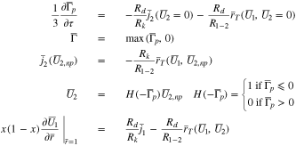
In a similar fashion to Case 2, Eq. 55 must be modified when ${R}_{1-2}=0$ to

$\begin{eqnarray}\begin{array}{rll}\displaystyle \frac{1}{3}\displaystyle \frac{\partial {\bar{{\rm{\Gamma }}}}_{p}}{\partial \tau } & = & -\displaystyle \frac{{R}_{d}}{{R}_{k}}\left({\bar{j}}_{1}\left({\bar{U}}_{1}=0\right)+{\bar{j}}_{2}\left({\bar{U}}_{2}=0\right)\right)+x\left(1-x\right){\left.\displaystyle \frac{\partial {\bar{U}}_{1}}{\partial \bar{r}}\right|}_{\bar{r}=1}\\ \bar{{\rm{\Gamma }}} & = & \max \left({\bar{{\rm{\Gamma }}}}_{p},0\right)\\ \displaystyle \frac{1}{3}H\left({\bar{{\rm{\Gamma }}}}_{p}\right)\displaystyle \frac{\partial {\bar{{\rm{\Gamma }}}}_{p}}{\partial \tau } & = & -\displaystyle \frac{{R}_{d}}{{R}_{k}}\left({\bar{j}}_{1}\left({\bar{U}}_{1}={\bar{U}}_{2}\right)+{\bar{j}}_{2}\left({\bar{U}}_{2}\right)\right)+x\left(1-x\right){\left.\displaystyle \frac{\partial {\bar{U}}_{1}}{\partial \bar{r}}\right|}_{\bar{r}=1}\\ H\left({\bar{{\rm{\Gamma }}}}_{p}\right) & = & \left\{\begin{array}{c}{\rm{0}}\,{\rm{if}}\,{\bar{{\rm{\Gamma }}}}_{p}\lt 0\\ {\rm{1}}\,{\rm{if}}\,{\bar{{\rm{\Gamma }}}}_{p}\geqslant 0\end{array}\right.\\ {\bar{U}}_{1} & = & {\bar{U}}_{2}\,{\rm{at}}\,\bar{r}=1\end{array}\end{eqnarray} \tag{ 57 }$

The dependent variables in Eq. 57 are ${\bar{{\rm{\Gamma }}}}_{p},\bar{{\rm{\Gamma }}},{\bar{U}}_{2}$ and the flux value $x\left(1-x\right){\left.\tfrac{\partial {\bar{U}}_{1}}{\partial \bar{r}}\right|}_{\bar{r}=1}.$ Again, the flux condition at $\bar{r}=1$ is replaced with a Dirichlet condition (the fourth of the above equations).

Equations 55 have a limited range of validity, as is the case for Eq. 53. To understand why, suppose one tried to use Eq. 55 in the situation given in Case 2, during charging, when the plated region is advancing toward the current collector. In such a situation, a point $\bar{z}$ might start out initially in the un-plated region, but over time become part of the plated region. In this situation, ${\bar{{\rm{\Gamma }}}}_{p}\left(\bar{z}\right)$ would become negative for the initial time period until the plated region reached $\bar{z}.$ These negative values would offset the resulting values for ${\bar{{\rm{\Gamma }}}}_{p}\left(\bar{z}\right)$ at all subsequent times, leading to false values for $\bar{{\rm{\Gamma }}}\left(\bar{z}\right).$ This problem does not arise in Case 3, because any point $\bar{z}$ that is initially un-plated remains un-plated for all subsequent times during which Eq. 55 are solved. The requirement that the plated region be receding in time is thus necessary for the validity of Eq. 55.

Some parameter relationships

The following relationships were used in solving the model equations. (See Ref. 16 and the Notation Index of this document).

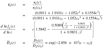
$\begin{eqnarray}\begin{array}{rll}{\bar{\kappa }}_{2}\left(c\right) & = & \displaystyle \frac{{\kappa }_{2}\left(c\right)}{{\kappa }_{2}\left({c}_{0}\right)}\\ & = & \displaystyle \frac{\left(0.0911+1.9101c-1.052{c}^{2}+0.1554{c}^{3}\right)}{\left(0.0911+1.9101{c}_{0}-1.052{{c}_{0}}^{2}+0.1554{{c}_{0}}^{3}\right)}\\ \displaystyle \frac{d\,\mathrm{ln}\,{f}_{\pm }\left(c\right)}{d\,\mathrm{ln}\,c} & = & c\left[1.5842-\displaystyle \frac{0.5089\left(\tfrac{1}{\sqrt{c}}-\tfrac{0.9831}{1+0.9831\sqrt{c}}\right)}{1+0.9831\sqrt{c}}\right]\\ {\bar{D}}_{2}\left(c\right) & = & \displaystyle \frac{{D}_{2}\left(c\right)}{{D}_{2}\left({c}_{0}\right)}=\exp \left[-2.856\,\times \,{10}^{3}\left(c-{c}_{0}\right)\right]\end{array}\end{eqnarray} \tag{ 58 }$

In the above formulas, $c=1000{c}_{2},$ that is, the units of $c$ are mol L⁻¹ where is the units of ${c}_{2}$ are mol cm⁻³.

Simulation Results and Discussion

Table I shows the parameter values used in simulations. At time $t=0,$ the half-cell started in an equilibrium state, in which ${U}_{1}={U}_{2}=0.6\,{\rm{V}}$ and ${c}_{2}={c}_{0}.$ A constant 1-C current was then applied to the cell^{^a} for a period of 2900 s. At this point, the cell was switched to open circuit and allowed to relax. Since little is known about the interfacial reaction 13 between the plated and intercalated lithium phases, the two extreme situations ${R}_{1-2}=0\,{\rm{or}}\,\infty$ were both simulated to explore how much of an impact this reaction can have on the onset of plating. The simulations were also done assuming a value of ${\bar{{\rm{\Gamma }}}}_{ref}={10}^{-3}\,{\rm{or}}\,{\bar{{\rm{\Gamma }}}}_{ref}=0.$ ^{^b} The equilibrium plots of Fig. 2 show the distinct near two-phase behavior of graphite associated with staging processes,^17–19 which is reflected in the non-equilibrium (1-C) plots we shall now discuss.

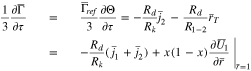
For the values ${R}_{1-2}=0\,{\rm{and}}\,{\bar{{\rm{\Gamma }}}}_{ref}={10}^{-3},$ Fig. 3a shows plots of the State of Charge (SOC) $x$ vs time at both the particle surface and the particle center. Two different positions in the electrode are shown for these plots: the separator interface at $\bar{z}=1$ and the current collector at $\bar{z}=0.$ In addition, the average state of charge over the entire particles at all positions $z$ within the electrode and the surface coverage of plated lithium ${\rm{\Theta }}=\bar{{\rm{\Gamma }}}/{\bar{{\rm{\Gamma }}}}_{ref}$ at $\bar{z}=1$ are also shown. Figure 3b shows corresponding plots of the voltages ${U}_{1}\left(\bar{r},\bar{z}\right)$ (shown at the particle surface $\bar{r}=1$ and the particle center $\bar{r}=0,$ for both the separator interface $\bar{z}=1$ and the current collector $\bar{z}=0$ ) as well as ${U}_{2}$ at both the separator interface and the current collector. Because ${R}_{1-2}=0,$ the plated and intercalated phases of lithium at the particle surface are equilibrated with each other and ${U}_{1}={U}_{2}$ at the particle surface, consistent with Eq. 47. Plating first occurs at the separator interface and, over time, extends backwards toward the current collector. The start of plating can be seen from the plot of ${U}_{2}\left(\bar{z}=1,t\right)$ at the separator interface, which drops below 1 mV at about 2600 s; note, however, that the precise onset of plating is not well defined when ${\bar{{\rm{\Gamma }}}}_{ref}={10}^{-3},$ because ${U}_{2}$ never completely becomes zero, but only tends exponentially to zero, as defined in Eq. 10. Equation 10 also implies that, at 1 mV, ${\rm{\Theta }}\approx 3.3,$ consistent with the plot of ${\rm{\Theta }}$ shown in Fig. 3a. Shown in Fig. 3b is the cell voltage ${V}_{cell}={{\rm{\Phi }}}_{1}\left(\bar{z}=0,t\right),$ which rises sharply at 2900 s, when the cell goes to open circuit.

**Figure 3.** The various curves are labelled according to their position coordinates $\left(\bar{r},\bar{z}\right):$ (a) compositions x at various positions and ${\rm{\Theta }}$ at the separator-electrode interface for ${R}_{1-2}=0$ , (b) cell voltage and potentials at various positions for ${R}_{1-2}=0$ , and (c) cell voltage and potentials at various positions for ${R}_{1-2}\,\to \,\infty$ vs time in s. The composition plot for ${R}_{1-2}\,\to \,\infty$ was very similar to that of Fig. 3a and, hence, is not shown.
Download figure:
Standard image High-resolution image

**Figure 3.** The various curves are labelled according to their position coordinates $\left(\bar{r},\bar{z}\right):$ (a) compositions x at various positions and ${\rm{\Theta }}$ at the separator-electrode interface for ${R}_{1-2}=0$ , (b) cell voltage and potentials at various positions for ${R}_{1-2}=0$ , and (c) cell voltage and potentials at various positions for ${R}_{1-2}\,\to \,\infty$ vs time in s. The composition plot for ${R}_{1-2}\,\to \,\infty$ was very similar to that of Fig. 3a and, hence, is not shown.
Download figure:
Standard image High-resolution image

At the start of open circuit, ${U}_{2}$ still remains close to zero at the electrode-separator interface, because the amount of plated Li there is still significant. It is only at about 2964 s that ${U}_{2}$ starts to rise rapidly at the electrode-separator interface, indicating that the plating has entirely dissolved, either into the graphite, the electrolyte, or both. By 3500 s, all of the curves have reached an asymptote, indicating that the cell is approaching an equilibrium state near 0.1 V vs Li. Figure 3c shows the same type of plots as Fig. 3b, but ${R}_{1-2}=\infty .$ Qualitatively, the plots are very similar, but the onset of plating occurs somewhat earlier, at around 2500 s, and the dissolution of the plating at open circuit takes somewhat longer, so that ${U}_{2}$ at the separator interface only starts to rise from zero at about 2976 s. At 3500 s, the cell again appears to be close to a state of equilibrium.

Figure 4a (for ${R}_{1-2}=0$ ) and Fig. 4b (for ${R}_{1-2}=\infty$ ) show the distributions of ${\rm{\Theta }}\left(z\right)$ at different times prior to the onset of plating. For both plots, ${\rm{\Theta }}\left(z\right)\lt 1$ indicating that underpotential deposition is taking place, but no significant amounts of plating are occurring. When the graphite galleries and the Li deposit are equilibrated (Fig. 4a, ${R}_{1-2}=0$ ), ${\rm{\Theta }}\left(z\right)$ reflects the staging behavior of the graphite substrate upon which the Li deposit resides. Conversely, when ${R}_{1-2}=\infty$ (Fig. 4b), the graphite galleries and the Li deposit are not equilibrated, and the additional resistance yields smoother ${\rm{\Theta }}\left(z\right)$ curves.

Figure 5a (for ${R}_{1-2}=0$ ) and Fig. 5b (for ${R}_{1-2}=\infty$ ) show the surface coverages ${\rm{\Theta }}\left(\bar{z}\right)$ after the start of plating, but prior to going to open circuit, for the cases when ${\bar{{\rm{\Gamma }}}}_{ref}={10}^{-3}$ and ${\bar{{\rm{\Gamma }}}}_{ref}=0.$ When ${\bar{{\rm{\Gamma }}}}_{ref}=0,$ the value $\bar{{\rm{\Gamma }}}/{10}^{-3}$ was plotted to enable better comparison with the ${\rm{\Theta }}$ -values plotted when ${\bar{{\rm{\Gamma }}}}_{ref}={10}^{-3}.$ The plots give some idea of how close the values calculated for ${\bar{{\rm{\Gamma }}}}_{ref}={10}^{-3}$ come to the limiting values when ${\bar{{\rm{\Gamma }}}}_{ref}=0.$ As previously noted, when ${\bar{{\rm{\Gamma }}}}_{ref}={10}^{-3}$ the onset of plating is not sharply defined, but when ${\bar{{\rm{\Gamma }}}}_{ref}=0,$ a clear boundary between plated and un-plated regions of the electrode can be seen, because in the un-plated regions $\bar{{\rm{\Gamma }}}\left(\bar{z}\right)=0.$

Figures 6a and 6b are similar to Figs. 5a and 5b, except in Fig. 6 the ${\rm{\Theta }}\left(\bar{z}\right)$ distributions are shown after the start of open circuit at 2900 s. Note that, whereas the plating occurred for 300 to 400 s before going to open circuit, the entire plated Li dissolves at open circuit within 70 to 80 s.

**Figure 6.** ${\rm{\Theta }}$ profiles after the start of open circuit at 2900 s, when ${\bar{{\rm{\Gamma }}}}_{ref}={10}^{-3}$ and ${\bar{{\rm{\Gamma }}}}_{ref}=0,$ for ${R}_{1-2}=0$ (a) and ${R}_{1-2}=\infty$ (b). In this figure, the boundary between the plated and unplated regions is receding in time, in contrast to Fig. 5. For the cases shown when ${\bar{{\rm{\Gamma }}}}_{ref}=0,$ the quantity $\bar{{\rm{\Gamma }}}/{10}^{-3}$ is plotted to compare with ${\rm{\Theta }}$ when ${\bar{{\rm{\Gamma }}}}_{ref}={10}^{-3}.$
Download figure:
Standard image High-resolution image

When ${\bar{{\rm{\Gamma }}}}_{ref}=0,$ there is a sharp boundary point at ${z}_{0}\left(t\right)$ between the plated and un-plated regions of the electrode, which can be determined as the plating advances due to lithiation (Case 2 of the equations) by determining the zero-crossing of the function ${\bar{U}}_{2,np}\left(t\right)$ (see the second of Eq. 53). At open circuit, when the plating recedes, ${z}_{0}\left(t\right)$ can be determined as the zero- crossing of ${\bar{{\rm{\Gamma }}}}_{p}$ in the first of Eq. 55. Figure 7 shows plots of ${\bar{z}}_{0}\left(t\right)$ for the cases ${R}_{1-2}=0$ and ${R}_{1-2}=\infty .$ Note that plating first occurs at the separator interface at $\bar{z}=1$ and then advances toward the current collector at $\bar{z}=0$ during lithiation. At 2900 s, when the cell goes to open circuit, the region of Li plating starts to recede toward the separator interface. Consistent with the prior discussion of Fig. 4, the results of Fig. 7 show that somewhat more lithium is plated when ${R}_{1-2}=\infty ;$ hence, for ${R}_{1-2}=\infty ,$ the plating starts earlier and takes longer to dissolve at open circuit.

**Figure 7.** Plots of the boundary ${\bar{z}}_{0}$ between the plated and unplated regions when ${\bar{{\rm{\Gamma }}}}_{ref}=0.$ In either case ( ${R}_{1-2}=0\,\mathrm{or}\,\infty$ ) plating always first starts at the electrode-separator interface ${\bar{z}}_{0}=1$ and progresses toward the current collector at $\bar{z}=0.$ After open circuit (dashed lines) the plating recedes, and the boundary ${\bar{z}}_{0}$ moves upward again toward the separator interface.
Download figure:
Standard image High-resolution image

**Figure 7.** Plots of the boundary ${\bar{z}}_{0}$ between the plated and unplated regions when ${\bar{{\rm{\Gamma }}}}_{ref}=0.$ In either case ( ${R}_{1-2}=0\,\mathrm{or}\,\infty$ ) plating always first starts at the electrode-separator interface ${\bar{z}}_{0}=1$ and progresses toward the current collector at $\bar{z}=0.$ After open circuit (dashed lines) the plating recedes, and the boundary ${\bar{z}}_{0}$ moves upward again toward the separator interface.
Download figure:
Standard image High-resolution image

When ${\bar{{\rm{\Gamma }}}}_{ref}=0$ and ${R}_{1-2}\gt 0$ there is a discontinuity in the function ${U}_{2}\left(z,t\right)$ when the cell switches to open circuit. The cell voltage jumps to a more positive value at the start of open circuit (see Figs. 3b and 3c at 2900 s), but the third and fourth of Eq. 55 imply that in the un-plated region of the electrode

$\begin{eqnarray}&&{\bar{j}}_{2}\left({\bar{U}}_{2}\right)=-\displaystyle \frac{{R}_{k}}{{R}_{1-2}}{\bar{r}}_{T}\left({\bar{U}}_{1},{\bar{U}}_{2}\right)\end{eqnarray} \tag{ 59 }$

The plating current density ${j}_{2}$ depends on the surface overpotential ${\eta }_{s,2}={{\rm{\Phi }}}_{1}-{{\rm{\Phi }}}_{2}-{U}_{2},$ and the jump in cell voltage forces a corresponding jump in ${U}_{2}$ in the un-plated region in order to preserve Eq. 59. In contrast, in the plated region of the electrode, ${U}_{2}$ must remain zero, both before and after going to open circuit. This results in discontinuities for ${U}_{2},$ both in time (at the onset of open circuit) as well as at ${z}_{0}$ (the transition point between the plated and un-plated regions). Figure 8a shows plots of ${U}_{2}\left(z\right)$ at various times after the onset of open circuit when ${\bar{{\rm{\Gamma }}}}_{ref}=0$ and ${R}_{1-2}=\infty ,$ where these discontinuities can be clearly seen. Figure 8b shows the same plots, but for the case when ${\bar{{\rm{\Gamma }}}}_{ref}={10}^{-3}.$ For any finite positive value of ${\bar{{\rm{\Gamma }}}}_{ref},$ the curves for ${U}_{2}\left(z\right)$ must be continuous, but they are clearly approaching a discontinuity for the small value ${\bar{{\rm{\Gamma }}}}_{ref}={10}^{-3}\ll 1.$ When ${R}_{1-2}=0,$ Eq. 59 no longer holds, because it is replaced with the equation ${U}_{2}={U}_{1}$ at $\bar{r}=1.$ Since ${U}_{1}$ remains continuous in both $t$ and $z,$ so must ${U}_{2}.$

**Figure 8.** If ${\bar{{\rm{\Gamma }}}}_{ref}=0,$ whenever ${R}_{1-2}\gt 0,$ the ${U}_{2}$ profiles in the electrode become discontinuous at open circuit at the boundary between the plated and un-plated regions. The upper panel (a) shows the case when ${R}_{1-2}\,\to \,\infty$ . Whenever ${\bar{{\rm{\Gamma }}}}_{ref}\gt 0,$ the ${U}_{2}$ profiles must be continuous, but one sees that at ${\bar{{\rm{\Gamma }}}}_{ref}={10}^{-3}$ (b) these profiles are tending toward the discontinuous behavior seen in the upper panel.
Download figure:
Standard image High-resolution image

**Figure 8.** If ${\bar{{\rm{\Gamma }}}}_{ref}=0,$ whenever ${R}_{1-2}\gt 0,$ the ${U}_{2}$ profiles in the electrode become discontinuous at open circuit at the boundary between the plated and un-plated regions. The upper panel (a) shows the case when ${R}_{1-2}\,\to \,\infty$ . Whenever ${\bar{{\rm{\Gamma }}}}_{ref}\gt 0,$ the ${U}_{2}$ profiles must be continuous, but one sees that at ${\bar{{\rm{\Gamma }}}}_{ref}={10}^{-3}$ (b) these profiles are tending toward the discontinuous behavior seen in the upper panel.
Download figure:
Standard image High-resolution image

The utility of differential voltage spectroscopy for determining the onset of Li plating,¹³ even at the 1-C charge rate, is demonstrated in Fig. 9. The peak associated with Li plating is less pronounced than for the equilibrium condition described in Fig. 2, but it is still quite evident. It is clear in Fig. 9 that when there is a sharp upturn in ${\rm{\Theta }}$ at the electrode-separator interface, corresponding to Li plating, there is also a peak in $\partial {V}_{cell}/\partial \bar{Q}.$ The origins of the peak are identical to those first described in this work in the context of Fig. 2, but the resistances reduce the magnitude of the peak at the 1-C charge rate.

**Figure 9.** ${R}_{1-2}=\infty$ and ${\bar{{\rm{\Gamma }}}}_{ref}={10}^{-3}.$ Cell voltage ${V}_{cell},$ its derivative $\partial {V}_{cell}/\partial \bar{Q}$ with respect to the dimensionless charge $\bar{Q},$ and the Li plating concentration ${\rm{\Theta }}={\rm{\Gamma }}/{{\rm{\Gamma }}}_{ref}$ at the electrode-separator interface. A key point in this figure is the peak in $\partial {V}_{cell}/\partial \bar{Q},$ reflecting the onset of Li plating, corresponding to the sharp upturn in ${\rm{\Theta }}$ at the electrode-separator interface.
Download figure:
Standard image High-resolution image

${R}_{1-2}=\infty $ — **Figure 9.** ${R}_{1-2}=\infty$ and ${\bar{{\rm{\Gamma }}}}_{ref}={10}^{-3}.$ Cell voltage ${V}_{cell},$ its derivative $\partial {V}_{cell}/\partial \bar{Q}$ with respect to the dimensionless charge $\bar{Q},$ and the Li plating concentration ${\rm{\Theta }}={\rm{\Gamma }}/{{\rm{\Gamma }}}_{ref}$ at the electrode-separator interface. A key point in this figure is the peak in $\partial {V}_{cell}/\partial \bar{Q},$ reflecting the onset of Li plating, corresponding to the sharp upturn in ${\rm{\Theta }}$ at the electrode-separator interface.
Download figure:
Standard image High-resolution image

Conclusions

We show how the model equations, previously developed in Refs. 1 and 2 for lithium plating, can be applied to examine a graphitic porous electrode and overcharge that leads to lithium plating. This previous work showed that the activity of plated Li on graphite cannot be set to one, as has been done up until now in previous literature,^3–14 because the first couple of monlayers of plating interact with the graphite and are thus thermodynamically different from bulk Li metal.

The resulting expression for the open-circuit voltage (OCV) as a function of surface coverage of plating, Eq. 10, is almost singular, that is, it is exponentially close to zero everywhere except for a very small surface coverage ${{\rm{\Gamma }}}_{ref},$ below which the OCV rises sharply. We illustrate the behavior of the near singular solutions to the porous-electrode equations, when ${{\rm{\Gamma }}}_{ref}$ is very small, corresponding to a couple of monolayers of lithium, and in the limiting case when ${{\rm{\Gamma }}}_{ref}=0.$ The latter case is of interest, because a precise value for ${{\rm{\Gamma }}}_{ref}$ is unknown.
During lithiation at constant current, once plating starts, there are two different regions of the electrode: the plated region near the separator interface and the un-plated complementary region adjacent to the current collector. When ${{\rm{\Gamma }}}_{ref}=0,$ different sets porous-electrode equations arise in each region. As the lithiation continues, the boundary between the plated and un-plated regions advances from the separator interface toward the current collector. A solution algorithm is given that simultaneously determines where this boundary is and solves the different sets of equations in each of these two regions.
If the Li plating process is abruptly interrupted, i.e., the cell is set to open circuit, the boundary starts to recede as plating is absorbed into the graphite. It turns out that the cases of advancing and receding boundary each require a different set of equations that must be solved when ${{\rm{\Gamma }}}_{ref}=0.$ We derive these different equations and illustrate solutions.
As was done in previous work,^1,2 an exchange reaction between plated and intercalated lithium at the surface of the graphite particles is also considered and characterized by a resistance ${R}_{1-2}.$ At this point in time, little is known about how large ${R}_{1-2}$ should be. We thus consider the two extreme cases, when ${R}_{1-2}=0$ and the plated lithium is always equilibrated with intercalated lithium at the particle surface, and ${R}_{1-2}=\infty ,$ when the plated and intercalated lithium can only exchange indirectly through the electrolyte. Although differences are seen between these two cases, the solutions are qualitatively very similar.
Solutions when ${{\rm{\Gamma }}}_{ref}=0$ are compared to solutions when ${{\rm{\Gamma }}}_{ref}$ is set to a small positive value, corresponding to about 2 monolayers of plated lithium. Here again, although differences between the two cases can be seen, they are qualitatively very similar.
Because of the singular nature of these equations, some details concerning the numerical solutions are included in an Appendix.

Appendix:: Some Details about the Numerical Simulations Shown

Figures 10a and 10b show the distributions of the local State of Charge $x\left(\bar{z},\bar{r}\right)$ and ${U}_{1}\left(\bar{z},\bar{r}\right)$ at the time $t=1435\,{\rm{s}}.$ Both of these figures exhibit some of the multi-phase behavior that is seen in the equilibrium plots of Fig. 2. Of particular note is the sharp drop in both $x\left(\bar{z},\bar{r}\right)$ and ${U}_{1}\left(\bar{z},\bar{r}\right)$ at about $\bar{z}=0.25.$ The drop is sharper at the particle center $\bar{r}=0$ than at the surface $\bar{r}=1,$ a trend which can also be seen in the plots of $x\left(\bar{z},\bar{r}\right)$ and ${U}_{1}\left(\bar{z},\bar{r}\right)$ at the surfaces and particle centers in Figs. 3a and 3b, although in Fig. 3, these drops are occurring in time, not in the spatial coordinates. As the amount of plated and intercalated lithium increases in the cell, the locations $\bar{z}$ of the sharp changes move through the cell, and this requires a very fine grid to avoid oscillations in numerical solutions. We note that the primary cause of these sharp changes is the staging behavior of the open-circuit voltage ${U}_{1}\left(x\right)$ for graphite (cf. Fig. 2), and the same phenomena occur when charging at rates as high 1-C, even without the presence of plating.

**Figure 10.** (a) Li filled sites in graphite as a function of position at $\tau =1.148,$ or 1435 s, about half way through the charge process and (b), the corresponding potential ${U}_{1}$ at the particle surfaces. From a numerical-computation perspective, the sharp gradients are of concern, as noted in the Appendix of this report.
Download figure:
Standard image High-resolution image

**Figure 10.** (a) Li filled sites in graphite as a function of position at $\tau =1.148,$ or 1435 s, about half way through the charge process and (b), the corresponding potential ${U}_{1}$ at the particle surfaces. From a numerical-computation perspective, the sharp gradients are of concern, as noted in the Appendix of this report.
Download figure:
Standard image High-resolution image

The equations were solved with the program Comsol using the Equation-Based Interface. A rectangular grid was used with 272 elements in the $z$ -direction and 68 elements in the $r$ -direction. A non-uniform mesh spacing in the $r$ -direction was used with a boundary layer near the particle surface. The BDF method²¹ for time stepping was used with a maximum BDF order of 5. For the case ${\bar{{\rm{\Gamma }}}}_{ref}={10}^{-3},$ the equations were also solved using a finite-difference code.¹⁶ The two different numerical solution methods produced results that were identical on the scales plotted in these figures.