
Abstract
The second part of this two-part study develops a systematic framework for parameter identification in polymer electrolyte membrane (PEM) fuel cell models. The framework utilizes the extended local sensitivity results of the first part to find an optimal subset of parameters for identification. This is achieved through an optimization algorithm that maximizes the well-known D-optimality criterion. The sensitivity data are then used for optimal experimental design (OED) to ensure that the resulting experiments are maximally informative for the purpose of parameter identification. To make the experimental design problem computationally tractable, the optimal experiments are chosen from a predefined library of operating conditions. Finally, a multi-step identification algorithm is proposed to formulate a regularized and well-conditioned optimization problem. The identification algorithm utilizes the unique structure of output predictions, wherein sensitivities to parameter perturbations typically vary with the load. To verify each component of the framework, synthetic experimental data generated with the model using nominal parameter values are used in an identification case study. The results confirm that each of these components plays a critical role in successful parameter identification.
Export citation and abstract BibTeX RIS

This is an open access article distributed under the terms of the Creative Commons Attribution 4.0 License (CC BY, http://creativecommons.org/licenses/by/4.0/), which permits unrestricted reuse of the work in any medium, provided the original work is properly cited.
Physics-based models of polymer electrolyte membrane (PEM) fuel cells have been extensively used to shed light on the underlying physical phenomena and optimize the cell design.1 However, in most cases, predictions by such models are only qualitatively valid2–5 and quantitative agreement with experimental data has remained mostly elusive. While the qualitative descriptions have proven useful in many cases, certain application areas, such as model-based control,6,7 require models with more predictive power. An important aspect of a model's prediction capability is the parameters used to run the model. Therefore, effective parameter identification is a critical step in developing quantitatively predictive models. Additionally, parameter identification is often used as a tool to infer a fuel cell's physical characteristics (e.g., catalyst activity or mass transport resistance) from experimental data8,9 and diagnose degradation,10 which further highlights the need for effective identification methods. Despite such a need, the parameter identification problem is relatively understudied in the fuel cell literature.11 This is an important gap that we aim to address in this work.
One of the main challenges associated with parameter identification in a large-scale model is that such models usually have a large number of parameters, many of which may not be practically identifiable given the available measurements. Under such circumstances, it is imperative to select a subset of parameters for identification.12 Particularly, the selected subset must only include parameters that can be identified using the available data. Moreover, the parameters must be selected in a way that ensures the predictive capability of the model is maintained.13
These are conflicting requirements that necessitate close inspection of output sensitivities to different parameters to ensure that the selected subset has the required characteristics. Accordingly, several methods have been proposed in the literature to ensure the selected subset is optimal.14–18 Among these, methods that optimize a scalar metric of the Fisher information matrix (FIM) to maximize the precision of parameter estimates are commonly utilized.18–20 Other approaches that directly focus on minimizing the model's prediction error have also been proposed.13,21 However, to date, these methods have not been applied to fuel cell models, which leaves significant room for improvements in model parameterization.
Another important aspect of parameter identification is the data used for this purpose. In particular, the data must contain enough information that allows the effects of different model parameters to be distinguished. The degree to which a data set is informative is controlled by the experimental conditions used to collect the data and the corresponding model sensitivities. Therefore, model-based experimental design approaches have attracted considerable attention in the literature.22–27 These techniques seek to find optimal experiments that are informative for parameter identification. This is done, for example, by using the model to find conditions that maximize the sensitivity of the predicted output to model parameters.28 Other proposed schemes maximize a scalar measure of the FIM,26,27 similar to parameter subset selection algorithms.
The idea of optimally designing experiments to reveal a parameter of interest is not new to the fuel cell community. Using differential conditions to achieve uniform distributions in a cell that allows characterization of membrane electrode assemblies (MEAs)29 and using low reactant concentrations to characterize the transport resistances9,30 are examples of this idea. However, these approaches are based on expert knowledge and are typically limited to specialized studies that focus on a particular behavior of the cell. Moreover, they are not guaranteed to be optimal for parameter identification. Therefore, there is a need to adopt the above-mentioned methods to fuel cell applications and rigorously optimize the experiments for effective model parameterization. We also note that recent battery literature has extensively utilized model-based optimal experimental design with considerable success, as evidenced by the improved parameter identification accuracy.31–36 This further highlights the potential benefits of using these methods for enhanced modeling of fuel cells, as many of the underlying equations are structurally similar to those used in battery models.
Once the subset of parameters to be identified is selected and the optimal conditions are used to collect the experimental data, the parameters can be identified. This last step is formulated as an optimization problem, whose solution typically minimizes the output prediction error of the model. Importantly, the structure of the available data can be utilized to improve identification results.28 Therefore, formulation of this step also requires consideration of model sensitivities to ensure the optimal solution is achieved. Here again, the fuel cell modeling literature is yet to capitalize on such potentials, leaving an important gap that should be addressed.
The above discussion points to several possibilities to improve parameter identification in fuel cell models. Accordingly, here we develop a systematic framework for effective model parameterization that addresses some of the current shortcomings of the fuel cell literature. While the framework is generally applicable to fuel cell models described by differential-algebraic equations, we use a pseudo-2D two-phase and non-isothermal model37–39 for this study as an example. Having investigated the sensitivities of various model predictions to different parameters in the first part of this work,40 here we focus on the problems of parameter subset selection and optimal experimental design. Particularly, we use our extended local sensitivity analysis results to select a subset of parameters for identification that is robust to initial assumptions about the nominal parameter values. We use similar procedures for robust optimal experimental design to obtain a set of experiments that are maximally informative for identification of the selected parameters. Finally, a multi-step parameter identification approach is proposed and tested with synthetic experimental data generated by the model.
The rest of the paper is organized as follows. First, a brief overview of the model and the considered parameters is given, where the first part of this two-part study is also reviewed. Next, the problem of parameter subset selection is addressed. The robust optimal experimental design procedure is then discussed followed by a description of the proposed identification algorithm. Lastly, the results for an identification case study are presented before closing with some concluding remarks.
Overview of the Model and Part I of the Study
In this work, we use a physics-based model that has been developed recently for automotive applications.37–39 Particularly, the model is pseudo-2D and captures non-isothermal and two-phase phenomena and has been extensively validated with performance and resistance data obtained experimentally from state-of-the-art fuel cell stacks.39 Further details about the model and its validation can be found in the original publications.37–39
The sensitivities of several of the model predictions to a variety of parameters were examined in the first part of this work using an extended local analysis.40 Particularly, cell voltage, high frequency resistance (HFR), and normalized membrane water crossover were studied for their sensitivity to 50 of the model parameters. The local analysis was conducted about several points in the parameter space to obtain a more global picture of the model sensitivities. Additionally, the sensitivities were generated using a large library of 729 different operating conditions with variations in temperature, pressure, relative humidity, and stoichiometric ratio. The parameters considered included geometrical and structural features of the cell, along with a number of fitting coefficients. The results were analyzed for sensitivity magnitudes and their relative independence, as they have implications for parameter identifiability. It was also demonstrated that many of the model parameters are not identifiable from cell-level measurements. This unidentifiability is often due to insensitivity of a parameter or multiple parameters having the same impact on the predicted outputs, which points to opportunities for model refinement, e.g., by re-parameterizing the model.41–43 It was further shown how additional measurements can enhance identifiability of model parameters by increasing their corresponding impact on the predicted outputs and reducing the correlation between the effect of different parameters (see the first part of the study for further discussion40).
Having analyzed model sensitivities, our exclusive focus in this part of the study is on parameter identifiability. Accordingly, we note that while we had considered 50 parameters for sensitivity analysis, many of these parameters, such as those describing the channel geometry, are known for a given stack. Although these parameters were included in our sensitivity analysis to ensure that our results are not constrained to a particular cell design, they are not suitable candidates for identification. Therefore, we narrow down the list of considered parameters in this part to focus on those that may be considered for model parameterization. Specifically, we limit our analysis here to a set of 31 parameters that are given in the Appendix Table A·I, which also provides the bounds for each parameter. Note that the specified bounds, which are determined based on the uncertainty of the corresponding parameters reported in the literature, ensure the parameters maintain their physical significance. Regarding the outputs of interest, here we assume that voltage and HFR are measured in the experiments as they often are in real-world testings. Therefore, our discussion here is based on the combined sensitivity of the voltage and HFR predictions. A summary of the sensitivity results is shown in Fig. 1 for the 31 parameters that are subject to this part of the study.
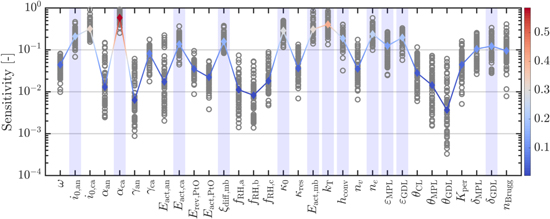
Figure 1. Summary of the sensitivity results based on voltage and HFR predictions and the results of the parameter subset selection method. The sensitivities at all sample points in the parameter space are shown as gray circles and the corresponding median is shown with the colored line, where the color changes based on the median sensitivity. The parameters selected by the robust parameter subset selection method are highlighted with a light blue shade.
Download figure:
Standard image High-resolution imageRobust Parameter Subset Selection
Attempting to identify all of the model parameters using only voltage and HFR data results in an ill-conditioned inverse problem.44 This necessitates the need for parameter subset selection so that the identification algorithm can focus exclusively on the parameters that are practically identifiable with the available measurements. We recall that a parameter is practically identifiable when it has an observable impact on the output predictions that is uniquely distinguishable from the impact of other parameters.17 Therefore, a large sensitivity magnitude alone does not guarantee identifiability of a parameter; the corresponding sensitivity vector must also be independent from that of other parameters. Accordingly, this section provides an algorithm that selects an identifiable subset of parameters. This subset selection procedure may also be viewed as a regularization technique to alleviate the ill-conditioning of the inverse problem.45,46 Briefly, the proposed method is as follows:
- 1.Inspect the parameter set for highly collinear pairs and remove the parameter with smaller sensitivity magnitude from such pairs.
- 2.Choose the number of parameters, nI, to be included in the subset. This is done using singular value decomposition.
- 3.Find the locally optimal subset of parameters at each point in the parameter space, for which sensitivity information has been calculated.
- 4.Find the globally optimal subset of parameters for the entire parameter space. The local solutions from the previous step are used to guide the optimization.
Below, each step is described in detail.
We start by inspecting the parameter sensitivities for highly collinear pairs. Given two sensitivity vectors  and
and  for parameters i and j obtained at point k in the parameter space, their collinearity index is defined as:
where  is the angle between the sensitivity vectors and the collinearity index
  varies between 0 and 1, indicating orthogonal and collinear sensitivity vectors, respectively. This collinearity index is calculated for all parameter pairs at all points in the parameter space, for which we had generated sensitivity data in the first part of the study.40 The median of the calculated indices is then used as the representative collinearity index for each parameter pair over the entire parameter space:

where k is the index for the sample point in the parameter space. Only one parameter from a pair whose median collinearity index is high can be practically identified.20 Therefore, for pairs with  exceeding a threshold value of ψth, the parameter with lower sensitivity magnitude is discarded. Here we use ψth = 0.9, which results in removal of i0,ca and Erev,PtO from the list of parameters due to their significant collinearity with αca and ω, respectively. We also note that a large threshold is chosen to ensure a certain degree of flexibility is maintained in the resulting set of parameters. More specifically, smaller thresholds can lead to removal of parameters that can have a noticeably different impact than their collinear counterparts only at a few selective operating conditions.
In the second step we determine the number of parameters, nI, that are needed to capture the variations in the data due to perturbations to the remaining parameters. Singular value decomposition47 is a powerful tool for this purpose. In particular, at each sample point in the parameter space we calculate the singular values of the sensitivity matrix. Let these singular values be ordered as follows:

where  denotes the i-th largest singular value of the sensitivity matrix obtained at the k-th sample point in the parameter space and nθ is the number of parameters under consideration after the lower sensitivity parameters in collinear pairs have been removed (nθ = 29). We then seek to find the smallest r such that:
where  monotonically increases with r and provides a qualitative measure as to how much of the total variations in the sensitivity directions are captured by the first r singular vectors. Moreover,
  is a threshold value that determines the number of selected singular values. Choosing a threshold of
  , we have found that, on average, 12 singular values are required to satisfy the above inequality at the sample points in the parameter space. Accordingly, we focus on selecting a subset of size nI = 12 for identification.
The third step of the algorithm is finding the locally optimal subset of parameters for identification. To this end, we must determine which of the model parameters have the largest unique impact on the predicted outcomes. This is done using the sensitivity matrix given by:

where  is the vector of output predictions and
  is the vector of parameters and the sensitivity matrix is evaluated at the k-th sample point in the parameter space. While our sensitivity calculations are slightly different,40 the structure of the resulting matrix is the same. To select a parameter subset, we want to choose columns of the sensitivity matrix that ensure the corresponding parameters can be identified with the required precision. The parameter estimation precision is determined by the corresponding covariance (
 ), which is constrained by the inverse of the FIM through the Cramer-Rao bound48:

where Fk is the FIM at the k-th sample point in the parameter space, which is given by:

Note that the definition of the FIM also includes the covariance of the measurement noise, which, for the subset selection procedure, can be assumed to be identity without loss of generality.20 With the Cramer-Rao bound and the FIM defined, we recall that the objective of this step is to select a subset of parameters, whose corresponding covariance is minimal. This can be achieved by minimizing the lower bound given by the FIM. To this end, a scalar metric of the FIM is optimized. A number of scalar metrics have been suggested based on different criteria.49 Among them, the D-optimality criterion is most commonly used,20 which maximizes the determinant of the FIM obtained from selected columns of the sensitivity matrix. Specifically, such an FIM is given by:
where L is the selection matrix defined as:

In the above equation,  denotes the jth standard unit vector and {i1, i2, ...,
  } is the set of selected parameter indices. We can now define the D-optimal selection criterion explicitly:

where  is the D-optimality criterion. The D-optimal solution,
  , maximizes the determinant of the FIM, which has the effect of minimizing the volume of the confidence ellipsoid for the parameter estimates. To find
  , an integer program must be solved20:
This is a combinatorial problem, whose solution may be obtained by exhaustive search for small problems.50 However, the search space grows combinatorially and this approach becomes infeasible even for moderately-sized problems. Therefore, clustering methods have been utilized to reduce the size of the problem.20,51 Optimization routines such as genetic algorithm (GA) may also be used, albeit with no guarantee of convergence to the true optimal solution.19 Alternatively, the popular orthogonal method14,52,53 can be used to obtain a sub-optimal solution. Particularly, Chu et al.18 showed that the orthogonal method is a forward selection algorithm that yields a sub-optimal solution for  . Forward selection in this context refers to the fact that at each iteration, the algorithm only picks the best parameter to be added to the already selected list of parameters. In that sense, the orthogonal method leads to a greedy algorithm.54 Variations of this algorithm have been suggested to consider multiple parameters at each stage, achieving more optimal results.18 The advantage of the original orthogonal method lies in its simple implementation. For example, the QR algorithm in MATLAB can be readily used for this purpose.14 Accordingly, we use the orthogonal method to find an initial sub-optimal solution that is then refined through GA.
Since only local sensitivity data are used in the above process, the resulting subset of parameters is only locally optimal and not applicable throughout the entire parameter space. A more robust approach is therefore needed. Two such approaches have been commonly used in the literature based on the R-optimality and ED-optimality criteria.26 In particular, the R-optimal selection criterion is based on a worst-case scenario and yields a selection that maximizes the minimum of the D-optimality criterion over the parameter space25,26:

On the other hand, the ED-optimality criterion maximizes the expected value of the D-optimality criterion over the parameter space24,26:

Either criterion may be used to select a robust subset of parameters that is less dependent on the nominal parameter values. We have found the R-optimality criterion to be sensitive to outlier points in the parameter space. Therefore, we use the ED-optimality criterion in this work. The corresponding optimization problem is an integer program similar to that presented in Eq. 11, which is solved using GA. In this case, the local solutions obtained during the previous step are used in the initial GA population to guide the optimization. The GA algorithm is run multiple times and the best solution is selected.
Using the procedure outlined in this section, we have selected a subset of 12 parameters for identification, which are highlighted in Fig. 1. The selected parameters cover a range of physical characteristics that impact the voltage and HFR predictions under a variety of operating conditions. For example, the selected subset includes parameters that impact the reaction kinetics, ohmic resistance, and mass transport losses. These are all parameters that may be inferred from voltage and HFR measurements alone. There are other parameters that could affect the internal conditions, but have no discernible impact on the measured signals, and therefore are not selected by the subset selection algorithm. Moreover, the selected subset may be affected by a range of modeler's decisions including the original parameter set considered (out of which a subset is to be selected), the bounds used for each parameter, and the operating conditions included in the predefined library. We also emphasize that this selection is optimal in an average sense, meaning that a better solution might exist in some regions of the parameter space. However, using the ED-optimality criterion helps ensure some degree of robustness to initial assumptions about the parameter values.
Robust Optimal Experimental Design for Parameter Identification
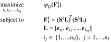
Having selected an identifiable subset of parameters, we now consider the experimental data used for identification. Importantly, we note that the data used for this purpose must be informative to ensure successful identification. This requirement motivates model-based optimal experimental design (OED), wherein the model is used to find the operating conditions that render the model predictions most sensitive to the parameters of interest. This idea is schematically shown in Fig. 2, where a numerical example is also illustrated.
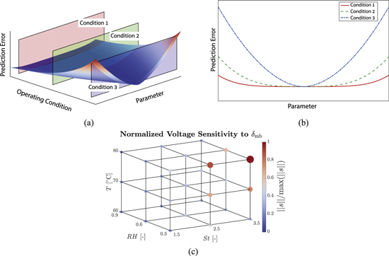
Figure 2. Optimal experimental design concept: (a) Schematic of model prediction errors as a function of parameter and operating condition, (b) schematic error variations with parameter for three example conditions, where the prediction error curve has a flat region for condition 1 rendering the parameter unidentifiable, while it is bowl-shaped for condition 3, which is ideal for parameter identifiability, and (c) example voltage sensitivities to membrane thickness, where hot and dry conditions are found to lead to increased sensitivity and improved identifiability of the membrane thickness.
Download figure:
Standard image High-resolution imageThe OED procedure requires solving an optimal control problem to obtain the most informative inputs. However, this approach is not computationally tractable for a large-scale model. Accordingly, methods such as input vector parameterization have been suggested,26 which searches over a discrete number of inputs to find the optimal solution. Alternatively, selecting an optimal set of conditions from a predefined library has been proposed as a computationally efficient method to solve the OED problem.32 Since we have generated sensitivity data for a library of conditions in part I,40 we use the latter approach to design maximally informative experiments for parameter identification.
Note that when working with a library of operating conditions, the OED problem is very similar to the parameter subset selection discussed earlier and the same procedures apply. Specifically, the sensitivity matrix obtained at the k-th sample point in the parameter space using the entire library of operating conditions consists of blocks that correspond to the individual experiments:

Here  denotes the sensitivity of the output predictions to the selected subset of parameters (set I) under the i-th set of operating conditions from the library of nl conditions. We recall that in this work we have nl = 729 conditions.
With the above block structure in mind, we note that while parameter subset selection is concerned with optimally choosing the columns of the sensitivity matrix to contain the most information, the OED focuses on choosing the best  blocks of the matrix for that same purpose. Therefore, D-optimality criterion is also commonly used for experimental design.22,32,35,36 The ED-optimality criterion may likewise be used for robust design.24,26 We note, however, that the orthogonal method is no longer applicable, since we are operating on the rows of the sensitivity matrix rather than its columns. Instead, the local D-optimal solution can be obtained through convex relaxation of the underlying integer program32:
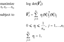
where nu is the experimental budget, i.e., the number of experiments to be selected from the library. Determining the experimental budget requires consideration of the actual experimental cost, as well as the computational cost required to evaluate the model for the selected experiments. Additionally, the number of selected experiments must provide enough information for parameter identification. Taking these into consideration, here we set the number of experiments to nu = 6.
The solution to the above convex program is a set of nu experiments that are D-optimal at sample point k in the parameter space. In other words, this solution is only locally optimal. Therefore, to find an experimental design that is less dependent on the initial parameter values, the ED-optimality criterion of Eq. 13 is used.
Briefly, the robust OED procedure is as follows:
- 1.Choose the number of experiments, nu, to be selected from the library.
- 2.Solve the convex program 15 to obtain the D-optimal design at the sampled points in the parameter space.
- 3.Use GA to obtain the ED-optimal design considering all of the sampled points. The D-optimal designs from the previous step are used in the initial population to guide the GA.
The experimental design resulting from this procedure is shown in Table I. The identification results based on this robust OED procedure are compared with another experimental design using Latin Hypercube Sampling (LHS). Importantly, we use the same number of experiments (nu = 6) for the LHS design. The resulting LHS design is given in Table II and the identified parameters using both experimental design procedures are compared below.
Table I. Robust optimal experimental design.
| Exp # | pch | Tcool | RHan | RHca | Stan | Stca |
|---|---|---|---|---|---|---|
| [bar] | [◦C] | [-] | [-] | [-] | [-] | |
| 1 | 2.5 | 80 | 30 | 30 | 2.5 | 2.0 |
| 2 | 1.5 | 80 | 30 | 90 | 1.5 | 2.0 |
| 3 | 1.5 | 40 | 90 | 90 | 2.0 | 2.5 |
| 4 | 1.5 | 80 | 90 | 30 | 2.0 | 2.5 |
| 5 | 1.5 | 80 | 30 | 30 | 2.5 | 2.0 |
| 6 | 1.5 | 80 | 90 | 30 | 1.5 | 2.5 |
Table II. Experimental design using LHS.
| Exp # | pch | Tcool | RHan | RHca | Stan | Stca |
|---|---|---|---|---|---|---|
| [bar] | [◦C] | [-] | [-] | [-] | [-] | |
| 1 | 2.68 | 59 | 80 | 72 | 2.3 | 2.1 |
| 2 | 2.05 | 48 | 54 | 51 | 2.3 | 1.5 |
| 3 | 1.79 | 62 | 65 | 43 | 1.8 | 2.2 |
| 4 | 2.85 | 70 | 85 | 83 | 1.7 | 1.9 |
| 5 | 3.33 | 75 | 48 | 32 | 2.1 | 2.5 |
| 6 | 2.45 | 43 | 33 | 62 | 1.5 | 1.7 |
Systematic Parameter Identification
So far, we have selected a subset of parameters for identification and designed informative experiments for that purpose. The last critical piece of the model parameterization framework is the identification algorithm. A good identification algorithm should be sufficiently constrained. An algorithm with too many degrees of freedom can lead to over-fitting and poor parameter identification.44 Regularization methods such as ridge regression45,46 and LASSO55 are commonly used to constrain the identification process and formulate a well-conditioned problem. However, in the context of parameter identification, application of these methods typically requires prior information about the parameter values. Since we assume no prior information about the parameters, here we focus on using the structure of the data to constrain the identification procedure. We also recall that the parameter subset selection approach, described above, indeed regularizes the problem to a certain extent and the identification algorithm of this section is developed for further regularization.
The underlying principle of the algorithm proposed here is that the cell response shows varying sensitivity to parameter perturbations depending on the load as seen in Fig. 3. For instance, a parameter that affects reactant transport resistance might only become identifiable at higher loads. Therefore, we use this particular sensitivity structure to identify the selected parameters in multiple steps. Particularly, we divide the polarization curve and the corresponding HFR data into 3 sections based on the load (see Fig. 3): (1) low current density or kinetic region, (2) medium current density or ohmic region, and (3) high current density or mass transport region. Alternatively, the regions may be defined based on the sensitivity data, for example, by classifying the regions based on average voltage sensitivity (low, medium, and high) under different conditions. However, here we utilize the existing knowledge in the fuel cell literature, where the three aforementioned regions are often well-defined. Encoding this knowledge into the framework allows for simpler formulation.

Figure 3. Sample output variations to changes in GDL porosity, where different load regions are identified. The sensitivity of the predicted outputs varies with the load.
Download figure:
Standard image High-resolution imageFollowing the above division, the selected parameters are grouped based on the corresponding sensitivities of the predicted outputs in each region. Specifically, the first parameter group consists of those parameters that are identifiable in the low current density region of the polarization curve, while the second and third groups include the parameters that become identifiable at medium and high current densities, respectively. Identifiability in this context is measured by the average output sensitivity to the parameter of interest; a parameter is deemed identifiable in a particular region if the corresponding sensitivity is greater than a threshold value Sth, which is chosen to be 0.1 in this work. This grouping procedure based on output sensitivities is shown in Fig. 4.

Figure 4. Combined voltage and HFR sensitivity for the entire library of operating conditions averaged among the samples in the parameter space. The blue, red, and gray bars denote, respectively, the parameters that are yet to be identified, those that are being identified in the current step, and those that were identified in a previous step and are being refined in the current step. The identifiability criterion is based on a sensitivity threshold that is chosen to be 0.1.
Download figure:
Standard image High-resolution imageFollowing the above grouping of parameters, the proposed multi-step identification algorithm is as follows:
- 1.Identify the parameters in the first group using data obtained at low current densities. The parameters in the other two groups are fixed at their nominal values.
- 2.Identify the parameters in the second group using data obtained at medium current densities. Parameters in the third group are kept at their nominal values, while those that were identified in the first step are further refined by allowing them to vary within a contracted search space.
- 3.Identify the parameters in the third group using data obtained at high current densities. Previously identified parameters are allowed to vary, but their respective search spaces are contracted. Particularly, the search spaces for the parameters in the first group are shrunken further compared to their ranges in the second step of the algorithm.
- 4.Refine all identified parameters using the entire data set. The search space for all parameters are further contracted in this step to constrain the problem. This step is only used to refine the identified values.
The general idea is that the output sensitivities to parameter perturbations typically increase as the load is increased. Therefore, it is helpful to start the identification process by only using the data at low current densities and as our confidence in the parameter estimates increases, move to higher loads and identify the remaining parameters. The increased sensitivity at higher loads also means that it is critical to allow previously identified parameters to be refined as the load is increased. Such cumulative fitting enables more accurate parameter estimation.31,32
Alternative implementations
Modified implementations of the general idea behind the presented multi-step identification algorithm are possible. A few potentially useful modifications are highlighted below:
- As we move to higher loads, our implementation disregards lower current density data points. Alternatively, one may use low current data at later stages of the identification algorithm along with larger weights for the higher current measurements (i.e., weighted least squares).
- In our implementation the problem is regularized by contracting the search space for previously identified parameters. Alternatively, the same effect may be achieved by penalizing deviations from previously identified parameters. For example, ridge regression or LASSO formulations can be utilized in later stages of the algorithm.
- We only group the parameters based on their sensitivity variations with the current density. Alternatively, this grouping can be carried out by considering all of the operating conditions, such as the humidity and temperature. However, even though this approach can lead to better regularized formulation, it would require more experimental conditions to be effective.
While we do not pursue any of the above modifications in this work, they offer some directions for further improvement of the proposed identification algorithm.
Verification of the Proposed Framework
As described above, the proposed model parameterization framework has three main components, namely, parameter subset selection, optimal experimental design, and the multi-step identification procedure. In this section, we demonstrate the utility of each of these components. To this end, we use the model to generate synthetic experimental data with a set of nominal parameter values ( ). The synthetic data are then used to identify the model parameters starting from perturbed values. Particularly, the optimization cost function is the weighted norm of the error:
where  and
and  denote the prediction error vectors for voltage (measured in mV) and HFR (measured in mΩ · cm2), respectively,
  and
and  are the number of elements in
  and
and  , and
, and  and
and  are the corresponding weights. Since the HFR varies in a smaller range compared to voltage, here we use
  = 1 and
  = 10. Given that we apply large perturbations to the nominal values and the above cost has many local minima, a gradient-based optimizer would fail to find the optimal solution. Use of a global optimizer is thus warranted. We have experimented with both GA and particle swarm (PS) algorithms and found that with the same level of effort to tune the optimizer hyper-parameters, the latter can find a more optimal solution. Therefore, we use PS to identify the selected parameters.
To highlight the importance of each part of the framework, we consider 4 different cases for identification:
- 1.
- 2.
- 3.
- 4.All parameters, except those that were removed during the collinearity analysis, are perturbed from their nominal values. The OED conditions (Table I) are used along with the systematic identification procedure to identify the parameters.
In all of the above cases, the applied parameter perturbations are random. In particular, the perturbations to the selected parameters are drawn from  (i.e., uniform distribution between −0.3 and 0.3), while the perturbations to the parameters that are not included in the identification (case 4) are drawn from
  . We also note that these perturbations are applied to the scaled parameter values and would amount to significant deviations from the nominal values on the original parameter axes. Additionally, it should be pointed out that the nominal values do not coincide with any of the sample points in the parameter space that are used to generate the sensitivity data, select the parameter subsets, and design the optimal experiments. These measures are taken to properly examine the robustness of the proposed framework.
The identified parameter values for the first two cases are provided in Table III along with the nominal and perturbed values. Moreover, the identification results for all of the above scenarios are shown in Fig. 5 in terms of the relative error of the identified parameters. Particularly, Fig. 5a compares the results from the first two scenarios and highlights the utility of OED. As seen in the figure, the maximum relative error in the parameter estimates is only 8.4% with the OED (for ne), whereas the LHS design results in a maximum relative error of about 170% (for ξdiff,mb). Moreover, the mean relative errors are 3.9% and 28.7% for the optimal and LHS experimental designs, respectively. In addition to these relative errors, the model voltage and HFR predictions are shown in Fig. 6. Particularly, the predictions with the nominal and identified parameter values are shown for both OED and LHS cases. Two main observations follow: first we note that the OED conditions lead to more pronounced variations in the predictions; therefore, they are more informative. Second, we observe that for both sets of conditions, the identified parameter values reproduce the synthetic experimental data very well. This result emphasizes that a good fit to experimental data does not readily imply an accurate parameter identification. These observations, combined with the relative parameter estimation errors mentioned above, demonstrate the importance of having maximally informative experimental data for parameter identification, which can be obtained through model-based OED.

Figure 5. Relative error in parameter estimates obtained using synthetic data. Case 1 is compared to case: (a) 2, (b) 3, and (c) 4 to demonstrate the effectiveness of optimal experimental design, the multi-step parameter identification algorithm, and the subset selection method, respectively.
Download figure:
Standard image High-resolution image
Figure 6. Polarization and HFR data obtained using OED and LHS conditions shown in Tables I and II, respectively. Results for both the nominal parameter values (markers) and the identified values (lines) are shown. The identified values are based on case 1 (for OED) and case 2 (for LHS) and are shown in Table III. Same axes limits are used to allow for direct comparison of the two experimental design results.
Download figure:
Standard image High-resolution image
Table III. Parameter identification results.
| Parameter | True | Perturbed | LHS | Robust OED |
|---|---|---|---|---|
| αca | 0.7 | 0.731 | 0.713 | 0.730 |
| i0,an | 0.01 | 0.002 9 | 0.010 9 | 0.009 3 |
| Eact,ca | 67.0 | 58.09 | 64.91 | 64.53 |
| ξdiff,mb | 1.0 | 0.317 | 2.698 | 0.997 |
| κ0 | 0.4 | 0.286 | 0.356 | 0.408 |
| Eact,mb | 15 | 13.54 | 14.97 | 14.54 |
| kT | 1.0 | 0.715 | 0.542 | 1.021 |
| hconv | 1.0 | 0.241 3 | 0.635 | 1.002 |
| ne | 1.8 | 2.166 | 1.387 | 1.649 |
| εMPL | 0.60 | 0.581 9 | 0.520 | 0.642 |
| εGDL | 0.78 | 0.754 | 0.674 | 0.722 |
| δGDL | 135 | 156 | 112 | 137 |
See Table A·I for parameter descriptions and units.
To show the effectiveness of the proposed multi-step identification algorithm, Fig. 5b compares the relative errors obtained using the proposed algorithm with those obtained from a single-step algorithm. The single-step algorithm uses the entire data set to identify all of the selected parameters. Note that in both cases we use the data based on OED conditions of Table I. The figure shows that the maximum and mean relative errors for the single-step case are 33.8% and 10.5%, respectively. This showcases the improved identification capability that is achieved by constraining the problem using the data structure.
Lastly, the subset selection approach is verified by comparing the identification results of case 1 with those of case 4, wherein the parameters that are not included in the selected subset are also perturbed from their nominal values. These results are shown in Fig. 5c. We note that if the subset selection algorithm is successful, then the parameters that are not included in the subset are not expected to have a significant impact on the output predictions. Therefore, perturbations to these parameters should not lead to considerable bias in the identified parameters. We further note that the parameters that were left out of the selected subset due to their collinearity with another parameter are not perturbed in case 4, as their perturbations can result in bias in the estimates of their collinear counterparts. As can be seen in the figure, perturbing the parameters outside of the selected subset does not have a significant impact on the relative errors in the parameter estimates. In particular, the maximum and mean relative errors are 11.6% and 3.8%, respectively, which are on par with those of case 1. Therefore, the subset selection algorithm has been successful.
These results highlight the importance of three key elements in successful parameter identification: selecting a suitable subset of parameters for identification, optimally designing experiments to generate maximally informative data for identification, and constructing a sufficiently regularized identification algorithm. Moreover, by extending the analysis beyond the vicinity of a point in the parameter space, these procedures can be made robust to initial assumptions about the nominal parameter values. We also emphasize that while a particular fuel cell model is used as an example to demonstrate the various steps involved in the parameter identification framework, the proposed procedures are generally applicable to different types of models, including other fuel cell models.
Since effective model parameterization is crucial to successful predictive modeling, these results can have profound implications for model-based design and control strategies. In addition, parameter identification plays a significant role in inferring physical characteristics of a fuel cell from experimental data. For example, parameter identification with cell-level measurements such as voltage has been used to diagnose fuel cell degradation issues,10 determine catalyst activity,8,56 and evaluate mass transport losses.9,30 Numerous electrochemical impedance spectroscopy (EIS) studies provide further examples of such efforts.57 Against this backdrop, the methods presented in this work also gain critical importance in further helping improve the current understanding of various aspects of fuel cell performance and durability by enabling more accurate parameter identification.
Summary and Conclusions
A framework for systematic parameter identification for PEM fuel cell models is developed. The framework consists of three main components: (1) selecting a robust subset of parameters for identification, (2) using model-based design of experiments to obtain a robust set of maximally informative data for identification of the selected parameters, and (3) using the structure of the data to formulate a regularized identification problem. This framework is based on the extended local sensitivity analysis that is explained in the first part of the study. Particularly, sensitivities of model predictions to parameter perturbations are used to determine the parameters that have the largest unique impact on the predicted outputs. This is formalized through the D-optimality criterion. Importantly, rather than maximizing the local D-optimality criterion, we maximize its expected value over a number of sample points in the parameter space to ensure the resulting subset is less dependent on the nominal parameter values. The same procedure is applied to select the most informative operating conditions from a predefined library of conditions. Lastly, a multi-step identification procedure is proposed to regularize the optimization problem. The effectiveness of each of the components in the framework is verified through a case study, wherein synthetic experimental data generated with nominal parameter values are used to identify the selected parameters. The results demonstrate the efficacy of the proposed subset selection, optimal experimental design, and the multi-step identification procedures in improving parameter identification results. While the methods of this work are applied to a full cell model, they can also be utilized for sub-models that focus on a specific phenomenon. Therefore, we believe that adoption of such methods would help ensure that the models are properly parameterized and their full predictive capabilities are realized.
Acknowledgments
Financial and technical support by Ford Motor Company is gratefully acknowledged.
Appendix
The complete list of model parameters considered in this work is provided below. Particularly, the parameter descriptions and their units and corresponding ranges are given. Importantly, note that all parameters considered here are bounded to specific ranges, which are determined based on the corresponding uncertainty in the parameter values reported in the literature.
Table A·I. Nomenclature and parameter list.
| Parameter | Description [Units] | Range |
|---|---|---|
| ω | Energy parameter for Temkin isotherm [kJ· mol−1] | [1, 20] |
| αan | HORa) transfer coefficient [-] | [1.2, 2.0] |
| αca | ORRb) transfer coefficient [-] | [0.4, 1.0] |
| i0,an | HOR exchange current density [A· cm−2] | [10−3, 10−1] |
| i0,ca | ORR exchange current density [A· cm−2] | [10−9, 10−6] |
| γan | HOR reaction order [-] | [0.5, 1] |
| γca | ORR reaction order [-] | [0.5, 1] |
| Eact,an | HOR activation energy [kJ· mol−1] | [5, 20] |
| Eact,ca | ORR activation energy [kJ· mol−1] | [30, 80] |
| Erev,PtO | Reversible potential for PtO formation [V] | [0.75, 0.85] |
| Eact,PtO | Activation energy for PtO formation [kJ· mol−1] | [5, 20] |
| ξdiff,mb | Scaling factor for membrane diffusivity [-] | [0.1, 10] |
| fRH,a | Fitting parameter for ORR RH dependency [-] | [0.4, 0.9] |
| fRH,b | Fitting parameter for ORR RH dependency [-] | [0.2, 4] |
| fRH,c | Fitting parameter for ORR RH dependency [-] | [0.3, 1] |
| κ0 | Factor for ionomer conductivity [S·cm−1] | [0.2, 0.6] |
| κres | Residual ionomer conductivity [S·cm−1] | [10−4, 0.006] |
| Eact,mb | Membrane conductivity activation energy [kJ· mol−1] | [5, 30] |
| kT | Scaling factor for thermal conductivity [-] | [0.1, 10] |
| hconv | Heat convection coefficient [W·cm−2 · K−1] | [0.05, 10] |
| nv | Saturation correction exponent for diffusivity [-] | [1, 3] |
| ne | Porosity correction exponent for diffusivity [-] | [1, 3] |
| Kper | Scaling factor for permeability [-] | [0.02, 50] |
| θCL | CLc) contact angle [◦] | [90.5, 100] |
| θMPL | MPLd) contact angle [◦] | [110, 150] |
| θGDL | GDLe) contact angle [◦] | [100, 130] |
| εMPL | MPL porosity [-] | [0.4, 0.65] |
| εGDL | GDL porosity [-] | [0.5, 0.85] |
| δMPL | MPL thickness [μm] | [20, 70] |
| δGDL | GDL thickness [μm] | [100, 240] |
| nBrugg | Bruggeman coefficient for CL [-] | [1, 3] |
a)Hydrogen Oxidation Reaction. b)Oxygen Reduction Reaction. c)Catalyst Layer. d)Microporous Layer. e)Gas Diffusion Layer.