Abstract
Building a complete cell impedance model and quickly calculating its frequency response are essential for battery design, optimization, and online management. Based on the widely accepted pseudo-two-dimensional (P2D) model, we build a complete full-order partial-dierential-equation (PDE) model for porous-electrode lithium-ion cells that includes a configurable electrical double-layer model at the solid-electrolyte interface (SEI). With the help of a numeric method, cell impedance and frequency responses of the cell's electrochemical variables at different locations inside the cell are obtained and analyzed. Moreover, in order to achieve the fast calculation of impedance and frequency responses, we derive transfer functions of the internal electrochemical variables, which give a set of exact closed-form equations for cell impedance and internal-variable frequency responses. The Nyquist plot results calculated by the closed-form equations are exactly consistent with the results of numeric simulations using the full-order model, which verifies the accuracy of the transfer functions and the effectiveness of the simplified method.
Export citation and abstract BibTeX RIS

This is an open access article distributed under the terms of the Creative Commons Attribution 4.0 License (CC BY, http://creativecommons.org/licenses/by/4.0/), which permits unrestricted reuse of the work in any medium, provided the original work is properly cited.
List of symbols
| A | surface area of the electrode, m2 |
| as | specific surface area of the porous electrode, m2 m−3 |
| c | concentration of lithium in phase indicated by subscript, mol m−3 |
| ce,0 | steady-state concentration of lithium in the electrolyte phase, mol m−3 |
| cs,max | maximum lithium concentration in an electrode particle, mol m−3 |
| cs,0 | initial concentration of lithium in the solid phase, mol m−3 |
| css | surface concentration of lithium in a spherical electrode particle, mol m−3 |

|
debiased version of css,  , mol m−3 , mol m−3
|
| Cdl | double-layer capacitance, F |
| De,eff | effective electrolyte diffusivity, m2 s−1 |
| Ds | solid diffusivity, m2 s−1 |
| f± | mean molar activity coefficient |
| F | Faraday's constant, 96 487 C mol−1 |
| iapp | applied cell current, A |
| ie | ionic current, A m−2 |
| is | electric current, A m−2 |
| j | reaction flux, mol m−2 s−1 |
| k | rate constant for the electrochemical reaction, molα−1 m4−3α s−1 |
| L | length of region of cell, m |
| r | radial coordinate, m |
| R | universal gas constant, 8.314 51 J mol−1 K−1 |
| Rct | charge transfer resistance, Ω m2 |
| Rdl | double-layer resistance, Ω m2 |
| Rfilm | film resistance, Ω m2 |
| Rs | particle radius, m |
| Rs,e | sum of the charge transfer resistance and the film resistance, Ω m2 |
| T | temperature, K |
| t+0 | transference number |
| t | time, s |
| Uocp | open circuit potential, V |
| v | cell voltage, V |
| x | l-d linear coordinate across the cell, m |
| z | normalized l-d linear coordinate across the electrode |
Greek
| α | charge-transfer coefficient |
| β |
parameter of Jacobsen–West transfer function:  . .
|
| ε | volume fraction of phase indicated by subscript |
| ϕ | potential of the phase indicated by subscript, V |

|
unbiased version of ϕ,  , V , V
|

|
solid-electrolyte potential difference, V |
| η | local overpotential, V |
| κeff | effective electrolyte conductivity, S m−1 |
| σeff | effective solid conductivity, S m−1 |
Subscript/superscript
| e | pertaining to the electrolyte phase |
| n | pertaining to the negative-electrode |
| p | pertaining to the positive-electrode |
| s | pertaining to the separator region |
| s | pertaining to the solid phase |
| fe | pertaining to the film/electrolyte interface |
| se | pertaining to the solid/electrolyte overall interface |
| sf | pertaining to the solid/film interface |
In recent years, with the advancement of transportation electrification, lithium-ion cells have undergone vigorous development.1–4 In order to understand and model their normal operation as well as their aging processes, the exploration of the internal mechanisms of lithium-ion cells is getting deeper and deeper.5–7 Electrochemical impedance spectroscopy (EIS) is a powerful tool that has been widely used to help visualize and understand the internal mechanisms in physical cells. However, because traditional experiments require a large quantity of material and time, it is now popular to use computer simulation of mathematical impedance models to make experimental design more efficient and reduce development costs.8 Impedance models can be used both for designing cells (e.g., evaluating potential electrode materials and geometries, understanding cell operation) and also for identifying cell-scale electrothermal model parameter values (e.g., for equivalent-circuit models and physics-based models) for a specific cell.9 These models may then be used by battery-management-system (BMS) algorithms to estimate state-of-charge (SOC), state-of-health (SOH), state-of-energy (SOE), and state-of-power (also known as state-of-function, SOF).10–13 Emerging applications also use impedance models for fault detection and temperature estimation.14 Therefore, an impedance model is invaluable for cell analysis and dynamics prediction.
This Paper introduces an exact closed-form impedance model for porous-electrode lithium-ion cells. It is based on the Doyle–Fuller–Newman (DFN) pseudo-two-dimensional (P2D) physics-based continuum-scale cell model, which has been widely recognized and applied for describing the internal physical processes and terminal-voltage responses of lithium-ion cells.15,16 The P2D model describes the operation of a lithium-ion cell using four partial-differential equations (PDEs) plus one algebraic closure term. However, when identifying a model for realistic lithium-ion cells, the solid–electrolyte interfacial model of the original P2D model turns out to be overly simplistic. Meyers et al.17 improved the P2D model by introducing a description of an electrical double-layer at the solid–electrolyte interface. Since then, a number of other electrical double-layer models have been proposed in the literature (e.g.,9,18–21), but no consensus regarding which is correct or "best" has yet emerged. The impedance model that we present is based on the work by Meyers et al. but is easily adapted to use other conventions.
If we consider the "input" to a battery cell to be its electrical current i(t) and the "output" from the cell to be the change in its voltage Δv(t) away from an equilibrium open-circuit voltage v0 as a response to that stimulus, then cell impedance is equal to the negative of the frequency response of the cell. That is, if v(t) = v0 + Δv(t) and so Δv(t) is the voltage drop over the cell internal impedance, then we can write in the frequency domain
where Z(ω) is the complex impedance at some frequency ω. The frequency response ΔV(ω)/I(ω) of the cell can be measured by injecting a small-amplitude sinusoidal current of frequency ω into the cell, and measuring the magnitude and phase change of the resulting small-signal sinusoidal voltage perturbation, from which the cell impedance function can be computed directly.
Many researchers have studied cell input/output impedance (e.g.,10,19,22), but we are not aware of any reporting research exploring the application of frequency response to study cell internal electrochemical variables (e.g., the electric potential in the electrolyte, the electric potential in the solid, the solid–electrolyte potential difference, the concentration of lithium in the electrolyte and solid, and the reaction flux). This may be because it is difficult to measure the frequency response of internal electrochemical variables by experimental means. (Frequency response has units of the output variable divided by units of the input variable. For this Paper, the input variable is always the cell's applied current, so the units of the divisor are always amperes. However, the units of the numerator of the frequency response depend on the variable being examined. Cell impedance considers the frequency response of the cell's terminal voltage, which has units of volts divided by amperes or ohms). Exploring the frequency response of internal electrochemical variables not only allows us to understand cells better, but also may bring new breakthroughs for state estimation and fault diagnosis. Utilizing a practical and straightforward identification method that calculates the impedance based on the input and output data of the improved P2D model in the time domain, we reveal the impedance and frequency response of the cell and internal electrochemical variables, which is a feature of this Paper.
While the full-order model (i.e. the PDE model) of a cell can be used to find its impedance response—as we will demonstrate later—the computational complexity of solving a set of nonlinear coupled PDEs makes the process very slow. For application to optimizing cell design iteratively via parameter perturbations or to adaptive parameter-identification approaches which also involve many iterated impedance calculations, it is valuable to have an exact closed-form impedance model for rapid calculations. A general approach to finding a closed-form impedance model is: (1) linearize the PDEs around an equilibrium (fixed state of charge and temperature) operational setpoint; (By definition, frequency responses exist only for linear systems, so this step is required). (2) take Laplace transforms of all linearized PDEs; and (3) combine these Laplace-domain equations to solve for the frequency response of interest. Sikha et al.21,22 obtained the impedance response in the "hyperbolic" form using similar steps but did not give the frequency response of all internal electrochemical variables. We give the solution process and results in the "exponential" form instead of the "hyperbolic" form in this Paper since we find that the numeric performance of the "exponential" form of solution at high frequencies is more robust in practice. That is, it is less sensitive to rounding errors. Smith et al.23,24 found frequency responses of the interphase potential difference ϕs − ϕe, the solid surface concentration cs,e, and lithium flux j. To do so, they not only linearized the PDEs in step (1), but found that they also needed to assume that the electrolyte potential was decoupled from the electrolyte concentration to form a solvable set of Equations. Lee et al. later25 extended this work to find frequency responses of the remaining internal electrochemical variables in the P2D model, but retained Smith's added assumption. More recently, Rodríguez et al.26 were able to find frequency responses for all of the electrochemical variables without the need to make the simplifying assumption, thus yielding an exact closed-form frequency response for the original DFN P2D model. However, this work did not consider the important electrical double-layer behaviors. In a work focused on developing frequency-response models for parameter-identification purposes, Chu et al.27 extended the work of Rodríguez to present a cell-level frequency response including the double layer, but written in terms of "lumped parameters" to facilitate parameter identification instead of in terms of DFN standard parameter descriptions. In this Paper, we use standard parameters to present an exact closed-form impedance model of a lithium-ion cell, including double-layer effects, and describing the frequency response of all internal electrochemical variables in addition to cell voltage. Most importantly, we verify that the transfer functions obtained according to our proposed simplified method can perfectly reproduce the small-signal frequency-response of the cell as verified through simulations of the full-order PDE models. These transfer functions of cell internal electrochemical variables are not only helpful for system-identification procedures,27,28 through further processing of model-order reduction techniques, but also can easily and reliably obtain the state-space model for online application.29 This Paper makes three main contributions: (1) it derives exact closed-form frequency responses for cell impedance and all internal electrochemical variables using a general electric double-layer model; (2) it demonstrates via comparison to small-signal numerical simulation of the full nonlinear PDE model that the closed-form solution matches the expected behaviors; and (3) it uses these results to propose methods to understand the frequency responses of internal cell variables to gain insight into cell performance, which might be useful—for example—when designing a new cell.
This Paper develops exact closed-form transfer function (impedance) models of internal electrochemical variables for porous-electrode lithium-ion cells. A previous work22 developed a comprehensive analytical model for a cell sandwich of dual-insertion electrodes that can be used to predict the cell's impedance response. Although similar in nature to the present work, reference22 focus on cell-level impedance modeling and connect the cell voltage impedance response to underlying electrochemical phenomena with a view toward parameter identification. Our work differs from theirs in that our interest is to obtain closed-form models of a variety of internal electrochemical variables in addition to the model for cell voltage. This is especially important to applications of reduced-order modeling and advanced cell-level control.29 Internal transfer function models are needed in order to generate the computationally compact forms that allow us to predict internal behaviors (in real-time) and ultimately guard against cell degradation through new control approaches. Clearly, since these quantities cannot be measured, we require accurate closed-form models. Additionally, we conjecture that such models will play an important role in constructing fully adaptive aging models using these techniques.
The remainder of this Paper is organized as follows: In Section Solid-electrolyte interface, a new double-layer model at the solid–electrolyte interface is proposed. In Section Improved P2D model, we describe the improved P2D model integrated with the double-layer model. In Section Impedance calculation using full-order model, we outline a method to obtain the impedance of the cell and internal electrochemical variables by a practical and straightforward impedance-identification method. In Section Interfacial impedance, we detail how to obtain the transfer functioof the interface. In Section Transfer function of electrolyte concentration and Transfer function of cell impedance, we present how the transfer functions of cell impedances and internal electrochemical variable impedances are obtained from the full-order model. In Section Result Comparison, we reveal and discuss the impedance results of cell and internal electrochemical variables, and compare the results of the transfer functions with the results of the full-order models. Finally, the summary is presented in Section Conclusions.
Full-Order Model
Solid-electrolyte interface
The original DFN P2D model was developed to describe constant-current (not transient) response. It ignores the double-layer of charge that builds up in the electrolyte at the solid–electrolyte interface, so some critical high-frequency cell behaviors can't be obtained. We introduce a more general model for this, as shown in Fig. 1a. In this Figure, ϕs is the electric potential in the solid, ϕsf is the electric potential in the solid–electrolyte interphase (SEI) film closest to the solid, ϕfe is the electric potential in the film closest to the electrolyte, and ϕe is the electric potential in the electrolyte. It can be considered that there is a particle/film interface (between ϕs and ϕsf), a film/electrolyte interface (between ϕfe and ϕe), and an overall interface (between ϕs and ϕe). Hence, in addition to the usual faradaic reaction flux, we assume that there may also be non-faradaic (capacitive) fluxes that develop from the charging and discharging of electrical double-layers at these interfaces. Because the double-layer of charge can be modeled as capacitance,17 we can model non-faradaic flux for any of these three interfaces as
where jdl is the non-faradaic reaction flux, Cdl is the double-layer capacitance, ϕ1 is the potential of the phase closest to the solid, and ϕ2 is the potential of the phase closest to the electrolyte.

Figure 1. Solid-electrolyte interface model (a) schematic diagram of double-layer (b) equivalent-circuit model (ECM) of interfacial impedance (c) simplified ECM of interfacial impedance.
Download figure:
Standard image High-resolution imageBecause the ions moving in the electrolyte also need to overcome resistance, we consider a more realistic double-layer model that includes a series resistance Rdl. In this case,
For cells where Rdl is considered to be negligible or nonexistent, we simply set Rdl = 0 in Eq. 2 to obtain the same result as Eq. 1.
Improved P2D model
After adding the solid-electrolyte interface details as described in Section Solid-electrolyte interface, the P2D model is refined as follows:
1. The governing Equation describing charge conservation in the solid is
having boundary conditions
where σeff is the effective electronic conductivity in the solid, ϕs is the electric potential in the solid, as is the specific interfacial surface area, F is the Faraday's constant, jf is the reaction flux from solid to electrolyte, A is the surface area, iapp is the cell applied current and x represents the 1-d cross-Section spatial location in the cell. Ln, Ls and Lp are the thickness of the negative-electrode, separator, and positive-electrode, respectively.
2. The governing Equation describing charge conservation in the electrolyte is
having boundary conditions,
where κeff is the effective electrolyte conductivity, ϕe is the electric potential in the electrolyte, R is the universal gas constant, T is the temperature,  is the transference number of the cation in the electrolyte with respect to the solvent, f± is the mean molar activity coefficient, and ce is the concentration of lithium in the electrolyte.
3. The governing Equation describing mass conservation in the solid is
having boundary conditions


where cs is the concentration of lithium in a spherical electrode particle, r is the coordinate in the radial pseudo dimension where r = 0 at the particle center and r = Rs at the particle surface, and Ds is the solid diffusivity.
4. The governing Equation describing mass conservation in the electrolyte is
having gradient boundary conditions,
and continuity boundary conditions,

where εe is the porosity and De,eff is the effective diffusivity of the electrolyte.
5. The Butler–Volmer closure term jf is
where the exchange flux density j0 and the overpotential η are defined respectively as


where k0 is the reaction-rate constant, cs,max is the maximum lithium concentration in the solid, css is the solid surface concentration, α is the charge-transfer coefficient, Uocp is the open circuit potential, and Rfilm is the resistance of the solid surface film.
Impedance calculation using full-order model
The set of partial-differential and algebraic equations in Sections Solid-electrolyte interface and Improved P2D model give the full P2D full-order model (FOM) of a lithium-ion cell. These equations will later be used to find an exact closed-form impedance model of the cell. First, however, we elaborate on how to obtain the impedance of the cell and the frequency responses of the internal electrochemical variables using a numeric time-domain simulation of the FOM.
Cell impedance is a function of frequency. It is defined for the case where cell applied current iapp is a sinusoidal excitation:

for  , where ω is the constant angular (radian) frequency of the excitation current, α is the amplitude of the excitation current, and t is time.
As described earlier, the impedance of a cell is equal to the negative of its frequency response. However, frequency responses, by definition, exist only for linear-time-invariant systems. The PDEs describing lithium-ion cell dynamics are nonlinear, but can be very closely approximated as linear perturbations around a constant setpoint v0 when the input current has small amplitude, which we will assume to be the case here. Under this assumption, the cell's perturbation-voltage response to the input-current stimulus will be a sinusoid having the same frequency as the input, amplified by factor  and phase shifted by arg G(jω). G(jω) is the "frequency response" or "frequency function" of the system, which gives full information to predict the output under the condition
  .
.
In a practical experiment, however, the current cannot be applied starting at time  . Instead, it is applied at some specific point in time that we reference as t = 0. In this case, the output will include an additional transient term that occurs due to the sudden application of the sinusoid at time zero. For example, the output voltage will be

where v(t) is the cell voltage and v0 is the at-rest initial open-circuit voltage.
To "measure" a frequency response, we will assume that measurement noises are zero mean and integrate to zero over one period of the input sinusoid, and further assume that the transient has decayed to zero before collecting data. Then, we can obtain the cell impedance from the output voltage according to the following steps, which are based on a Fourier-series analysis method.
First, we define
where T represents the period of the excitation current.
Substituting Eq. 22 into Eqs. 23 and 24, we have
We can get the magnitude response  and the phase response
  by combining Icos(ω) and Isin(ω),

Finally, we obtain the cell impedance Z(jω)
In Section Result Comparison, we will use this method to calculate cell impedance numerically. Similarly, the proposed method is also applicable to find the frequency responses of the electrochemical variables inside cells, such as the electric potential in the electrolyte ϕe and in the solid ϕs, the solid-electrolyte potential difference  , the concentration of lithium in the electrolyte ce and at the solid surface css, and the reaction flux j. That is, the frequency-response information of internal electrochemical variables also can be obtained simply by replacing the cell voltage v(t) in these equations with these variables.
Transfer Function
In Section Full-order Model, we introduced the full-order PDE-based enhanced P2D model of the dynamics of a lithium-ion cell. We will assume that this model is a faithful representation of cell dynamics, and so numeric simulation of this model will give accurate predictions of internal and external cell responses to input stimuli. However, solving PDEs is a time-consuming process and not ideal for use inside optimization loops (such as when optimizing cell designs or optimizing parameter values to fit model predictions to measured values for a physical cell) or for use in real-time battery-management-system applications.
In this Section, we show a way to find exact closed-form frequency responses corresponding to this full-order model. The process is to linearize and combine all PDEs, boundary conditions and initial conditions, and then to solve for individual frequency responses after Laplace transformation. Our goal is to obtain the transfer functions and frequency responses of the interface impedance, the internal electrochemical variables, and the cell impedance. The procedure is largely the same as the one presented by Rodríguez et al.26 but now allowing the ability to include a general solid–electrolyte interfacial impedance model, possibly including a very general electric double-layer description. In this Paper, we focus on the steps needed to generalize the method of Rodríguez et al. to find cell impedance; the Appendix gives solutions for the transfer functions of all other internal variables.
Interfacial impedance
Impedance at particle/film interface
The primary distinction between the process followed in this Paper to create frequency responses and the process presented by Rodríguez et al. is that we have modified the procedure to allow for a more general model of the solid–electrolyte interface, including the possibility of one or more electrical double layers at the interface. The flowchart presented in Fig. 2 illustrates the revised process, where the most significant change is to the steps required to find this interfacial impedance model and to the resulting expression for this impedance. The position of these new steps in the overall method for finding all transfer functions is illustrated by the top-right box labeled "Interfacial impedance model". Following the determination of this new impedance model, similar steps to those used by Rodríguez et al. are used to derive a transfer function for perturbations to the electrolyte concentration caused by applied electrical current, where the only modifications to the derivation are to allow use of this new general impedance model vs the specific impedance model previously assumed. Once the electrolyte-concentration transfer function is obtained, there are no additional changes in the procedure followed to find the remaining cell transfer functions, which are all dependent on the electrolyte-concentration transfer function. In the Figure, the blue boxes represent time-domain Equations, the yellow boxes represent frequency-domain equations leading up to the electrolyte-concentration transfer function, and the green boxes represent frequency-domain equations resulting from the electrolyte-concentration transfer function.
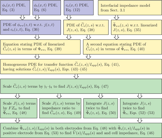
Figure 2. Flowchart illustrating the process for finding all transfer functions.
Download figure:
Standard image High-resolution imageWe begin to see how to include the electrical double-layer model by investigating impedance at the particle/film interface in the frequency domain. According to the solid-concentration PDE stated in Eq. 9 and the conversion approach from the time domain to the frequency domain derived by Jacobsen and West,30 we can obtain the transfer function  as
as
where  , css(t) is the concentration of lithium at the surface of the solid and cs,0 is the initial equilibrium concentration of lithium in the solid.
  and
and  are the representations of
  and
and  in the Laplace frequency domain, respectively, "s" is the Laplace generalized frequency variable, and
  is the faradaic reaction flux from solid to film,
  .
.
We can solve for  by linearizing the Butler–Volmer Equation for this interface and taking the Laplace transform of the result. First, we form a Taylor-series expansion around the linearization setpoint

where ce, 0 is the equilibrium electrolyte concentration, and discard higher-order terms. This gives
where  , and
, and 
 .
.
Rearranging, we get
where  . Taking the Laplace transform,
We define ideal particle-diffusion impedance Zs,
Then, combining Eqs. 31 and 30, we have

In addition to the faradaic flux, the interface supports a non-faradaic flux according to Eq. 2
Taking the Laplace transform of this relationship, we have

The interface supports a total flux
where Ysf is the admittance of the solid/film interface and Zsf = 1/Ysf.
Impedance at film/electrolyte interface
In this subsection, we investigate impedance at film/electrolyte interface. Our methods and steps to solve for  are similar to those used to solve for
  . At this interface, we ignore any variation of the open-circuit potential of any reaction occurring at the film/electrolyte interface due to variation in the concentration of lithium in the film or solution (this is the same assumption as made by Meyers et al.17).
Following the same method as before, we find
where  and
and  is the reaction flux from film to electrolyte,
  .
.
Again, the interface also supports a non-faradaic flux according to Eq. 2
Taking the Laplace transform, we have

The interface supports a total flux
where Yfe is the admittance of the film/electrolyte interface and Zfe = 1/Yfe.
Overall interfacial impedance model
We now combine these results to find an expression for the impedance of the overall interface. First, the resistance of the film is considered to be purely ohmic,

Second, we recognize that the total flux through every one of the interfaces considered so far must be equal. Therefore, Jsf = Jfe = Jse. Therefore, Eqs. 31 and 33 can be written as
Adding Eqs. 31, 33, and 34, we get

The interfacial impedance model is nearly complete: all that remains is to consider the double layer between ϕs and ϕe, which is modeled according to Eq. 2 as
Taking the Laplace transform, we have

So the total molar flow rate from solid to electrolyte is
Defining debiased solid-electrolyte potential difference  , we find the transfer function of the interface to be

where
This interfacial model can be visualized using the equivalent circuit shown in Fig. 1b. The reader can verify that linear-circuits principles applied to analyze this circuit will yield the same overall impedance Zse as found by the rigorous derivation just presented based on the PDEs themselves. Therefore, the circuit is a very helpful tool for visualizing how the individual impedances contribute to the overall impedance of the interface. We also note that this interfacial model is more general than we are likely to need. In particular, it is difficult to identify all the model parameter values corresponding to a physical cell. Instead, in the remainder of this Paper we use the simplified version of the interfacial impedance model shown in Fig. 1(c) which is achieved by setting  , and
, and  . For this model, Zse = Zsf + Rf.
Transfer function of electrolyte concentration
Now that the interfacial impedance Zse has been derived, the next step is to use its value in the development of a transfer function for the electrolyte concentration. The process that we follow here is identical to that of Rodríguez et al.26 except that we must substitute this different interfacial impedance at the correct point in the derivation.
We begin by subtracting Eq. 6 from Eq. 3 to obtain the PDE of solid-electrolyte potential difference
Until now, we have used natural spatial variable x; we now begin to use normalized spatial variable z to describe the one-dimensional span of the electrode (location z = 0 represents the location at the current collector; location z = 1 represents the location at the electrode/separator boundary).
We define the debiased electrolyte concentration as  . Linearizing using a Taylor-series expansion, we have,
So Eq. 36 becomes,
After taking the Laplace transform of both sides of this Equation, we have
We also take the Laplace transform of Eq. 12,
Substitute Eq. 38 into 37, to get
At this point, we are ready to substitute the result of the new interfacial impedance Equation. We combine Eqs. 35 and 38, to find
Because  , we can combine Eqs. 39 and 40
Rearranging, and dividing by Iapp(s), we have
where
This is exactly the same form of solution as found by Rodríguez et al. except for a slightly different definition of τ1(s) and τ2(s) to accommodate the generalized interfacial impedance model. From this point on, the derivation is identical to that in the earlier work, using these revised definitions of τ1(s) and τ2(s). In particular, the generic solution is
where
So, the solution in the negative electrode is
Because js(z, t) = 0 and  does not exist in the separator region, the solution in the separator becomes
The solution in the positive electrode is
In order to find the specific solution, the coefficients  ,
,  ,
,  ,
,  ,
,  ,
,  ,
,  ,
,  ,
,  , and
, and  , must be found to satisfy the boundary conditions of the problem. The method and even the closed-form equations for doing so are identical to those in,26 except for the different definitions of τ1(s) and τ2(s). These equations are listed in the Appendix for completeness. The transfer functions of other electrochemical variables derived based on
  are also listed in the Appendix. Note that in these Equations, the superscript "n" denotes negative electrode, "s" denotes separator, and "p" denotes positive electrode.
Transfer function of cell impedance
After obtaining the transfer functions of all electrochemical variables, we can build a full-cell impedance model. Using the solid potential at the positive and negative current collectors (where z = 0), we have,
Because our transfer functions compute  and not
  directly and because the biasing term is cell voltage itself in the positive-electrode, so we cannot use the transfer functions for
  to find cell voltage. Instead, we write
  , so
, so
We define debiased (linearized) voltage
since, by definition,  . Then, we can take the Laplace transform of
  to get the transfer function
This is an exact closed-form result for the frequency response of a lithium-ion battery cell, based on the assumed PDE model.
Note that an impedance understanding of a cell writes
So, we can write the cell impedance using transfer functions as
since  .
.
Result Comparison
Here we demonstrate that the closed-form frequency response functions developed for cell terminal voltage and cell internal electrochemical variables indeed match small-signal numerical simulation of the full PDE model. What follows are simulation results –clearly it is not possible to perform a meaningful comparison using a physical cell because: (1) a cell's physical parameters are not known exactly, and so any difference between a measured cell response and a response predicted by the closed-form frequency responses could not be explained without uncertainty, and (2) it is not possible to measure frequency responses for cell internal electrochemical variables in situ.
However, assuming that the DFN P2D model—along with an integrated interfacial impedance model—adequately describes the dynamics of a physical cell, the results of this Paper can be used to characterize essential internal and external behaviors of that physical cell. Importantly, an accurate internal model can predict critical electrochemical aspects affecting cell performance. For example, by modeling electrode surface overpotential, it is possible to anticipate –and through controls mitigate –the plating of metallic lithium. The occurrence of such effects can be detected using a number of non-destructive methods31 and formally verified by post-mortem examination, lending confidence to the use of the internal models.
In this Section, we first numerically simulate the full-order PDE model with a small-signal sinusoidal input and then use the method of Section Impedance calculation using full-order model to calculate the cell impedance as well as the individual frequency responses corresponding to internal cell variables from the numeric simulations. We also examine the closed-form frequency-responses and show that there is complete agreement among the results computed using either method.
Cell impedance results
We begin by examining overall cell impedance response. For the full-order model, we solve the PDEs in Section Improved P2D model using COMSOL commercial software in the time domain, simulating the cell's voltage response to 200 periods of an input-current sinusoid to allow time for the output transient to decay to a negligible level. We refined the FEM mesh until results were mesh independent: a very fine mesh was required for the 2-d domain on which the solid concentration was evaluated (600 elements per electrode), which resulted in slow simulations, with median simulation time of over 20 minutes per frequency on a computer having 16 Gb RAM and a multicore 2.8 GHz Intel i7 processor. The model parameter values were chosen from the widely reported Doyle–Fuller–Newman (DFN) set,15 and are listed in Table I. The cell SOC is set to 80%. To show that the proposed approach works both with and without an electrical double-layer model, an electrical double layer was included in the negative electrode (by adding the appropriate parameters to the standard DFN set) but not in the positive electrode (by setting those parameter values to zero). The angular frequency range of the cell applied current iapp was set to 10−4 ∼ 103 rads−1 (that is 1.59 × 10⁻⁵ ∼ 159 Hz), with six frequency points per decade. The amplitude value of the cell applied current iapp was set to 0.001 A. After the COMSOL simulations, one period of output voltages corresponding to several different exemplary input-current angular frequencies are shown in the magenta curves in Fig. 3a. Then we used the impedance-identification method described in Section Impedance calculation using full-order model to obtain the Nyquist plot of cell impedance. The results are shown as a dotted curve in Fig. 3b. To verify the correctness of the proposed impedance-identification method, the results of  and
and  are returned to Eq. 22. The resulting voltages are shown in the blue curves in Fig. 3a, and are consistent with the simulation voltages, so correctness of the methodology is verified.

Figure 3. Cell impedance.
Download figure:
Standard image High-resolution imageTable I. Cell parameters for the simulation.
| Symbol | Units | negative-electrode | Separator | positive-electrode |
|---|---|---|---|---|
| L | μm | 128 | 76 | 190 |
| R | μm | 12.5 | — | 8.5 |
| A | m2 | 1 | 1 | 1 |
| σ | S m−1 | 100 | — | 3.8 |
| εs | m3m−3 | 0.471 | — | 0.297 |
| εe | m3m−3 | 0.357 | 0.724 | 0.444 |
| brug | — | 1.5 | — | 1.5 |
| cs,max | mol m−3 | 26 390 | — | 22 860 |
| ce,0 | mol m−3 | 2000 | 2000 | 2000 |
| θ0 | — | 0.05 | — | 0.78 |
| θ100 | — | 0.53 | — | 0.17 |
| Ds | m2 s−1 | 3.9 × 10⁻¹⁴ | — | 1.0 × 10⁻¹³ |
| De | m2 s−1 | 7.5 × 10⁻¹¹ | 7.5 × 10⁻¹¹ | 7.5 × 10⁻¹¹ |
| t+0 | — | 0.363 | 0.363 | 0.363 |
| k0 | mol−1/2 m5/2 s−1 | 1.94 × 10⁻¹¹ | — | 2.16 × 10⁻¹¹ |
| α | — | 0.5 | — | 0.5 |
| Rf | Ω m2 | 0.0 | — | 0.0 |
| Rdl | Ω m2 | 0.0 | — | 0.0 |
| Cdl | F m−2 | 100 | — | 0 |
| dln f±/dln ce | — | 3 | 3 | 3 |
We compute σeff = σεs, κeff =  , De,eff =
  .
.
In the electrolyte, conductivity is a function of concentration (here, evaluated at ce,0):
 +
+  +
+  −
− 
For the negative-electrode, the open-circuit potential function is:
 =
=  +
+ 
For the positive-electrode, the open-circuit potential function is:
 =
=  −
− 
![$-\ 0.0275479\left[\displaystyle \frac{1}{{\left(0.998432-\theta \right)}^{0.4924656}}-1.90111\right]$](https://content.cld.iop.org/journals/1945-7111/167/1/013539/revision1/jesab67c7ieqn71.gif) +
+ ![$0.810239\exp \left[-40(\theta -0.133875)\right].$](https://content.cld.iop.org/journals/1945-7111/167/1/013539/revision1/jesab67c7ieqn72.gif)
We also computed cell impedance using the closed-form frequency responses using the method presented in Section Transfer function of cell impedance. To do so, we used the same cell parameter values that were used for the numeric method. Because the transfer functions have low computational complexity, we computed frequency responses for 200 frequencies over the desired frequency interval. The Nyquist plot of cell impedance obtained from the transfer function are shown as a solid curve in Fig. 3b. We see that the results are consistent with the results of the full-order models. This validates the accuracy of the transfer functions and the effectiveness of the proposed method for simplifying the full-order models.
The overall computation time required by the COMSOL PDE simulations was over 10 h to compute cell impedance and all internal-variable frequency responses for a total of 31 distinct frequencies at the level of numeric accuracy needed for comparing with the transfer-function approach. In contrast, the transfer-function approach found all cell impedances for 200 distinct frequencies in a total of 5 ms using unoptimized MATLAB code on the same computer; it found all electrochemical-variable frequency responses for the same 200 frequencies in 86 ms total. This points out two benefits of the transfer-function approach: (1) it is enormously faster (on the order of 45,000,000 times faster for cell impedance at a single frequency); (2) the transfer-function approach allows computing frequency responses for only the set of variables desired, while the PDE simulation must compute all frequency responses together.
Electrochemical variable impedance results
Using the closed-form transfer functions, we obtain Nyquist plots of twelve internal electrochemical variables computed for different locations within the cell electrode. Positive and negative electrode results for electrolyte concentration, solid surface concentration, reaction flux, electrolyte potential, solid potential, and solid-electrolyte potential difference are shown in Fig. 4, through Fig. 9, respectively. The dotted curves denote results obtained from COMSOL numeric simulation of the full-order models; the solid curves are those obtained directly from the transfer functions. Different colors represent different locations within the electrode (again, location z = 0 represents the location at the current collector; location z = 1 represents the location at the electrode/separator boundary). We see here that the results for the internal transfer functions exactly match the results of the full-order models. This further validates the accuracy of the closed-form transfer functions and, importantly, suggest their potential effectiveness in simplifying the full-order models for use in real-time controls. Next we present the frequency responses of each electrochemical variable and briefly describe their characteristics. Note that with the exception of electrolyte potential, the Nyquist plots for variables computed at negative and positive electrodes appear in alternate quadrants of the complex plane. This is due to the reversal of polarity with respect to the applied current for the associated electrode which brings about a 180 degree phase shift.
Frequency response analysis
Frequency responses computed from transfer functions can convey important information about underlying system dynamic behavior. Applied to batteries, we normally consider electrochemical impedance spectroscopy (EIS) and confine our analysis to a spectral characterization of cell output voltage in relation to input current. But this technique examines an external measures only and is thus limited in what it can reveal internal to the cell's electrochemistry. The present work expands the scope of standard analysis by enabling the calculation of individual frequency responses for internal electrochemical variables computed at various locations within the cell.
Frequency response of electrolyte concentration
Nyquist plots for the concentration of lithium in the electrolyte are shown in Fig. 4. The different colors represent frequency responses computed at different locations across the electrode. Since the transfer function model created in Sections Solid-electrolyte interface to Improved P2D model is not a rational function, we are not able to perform meaningful analysis directly (e.g., via pole-zero determination). Nonetheless, the computed frequency responses afford us the ability to observe certain aspects of the underlying behavior.

Figure 4. Frequency response of the concentration of lithium in the electrolyte.
Download figure:
Standard image High-resolution imageElectrolyte concentration Nyquist plots are clearly dominated by a first-order characteristic for all anode locations; this is representative of a diffusion process, which in the present case reflects both bulk diffusion of lithium ions through the electrolyte as well as through the porous structure of the electrode. The dominant time constant may be found as the reciprocal of the radial frequency associated with the largest magnitude imaginary component of the principle semicircle. Careful analysis of the frequency response indicates that this frequency is consistent for all locations and is found to be  which gives a corresponding diffusion time constant
  . Note that the actual frequency response deviates from the ideal first-order at both high and low frequency ranges indicating processes not modeled by first-order diffusion. Generally speaking, the Nyquist plot for the cathode exhibits the same essential features seen at the anode –i.e. dynamics are dominated by a first-order diffusion process. In this case, measurements show the dominant time constant varies slightly from
  at the current collector location to
  at the electrode surface. The key difference noted between the two electrodes is a reversal of sign which introduces a 180 degree phase shift to the plot, as we expect due to the reverse of polarity.
Frequency response of reaction flux
Nyquist plots of reaction flux are shown in Fig. 5. The individual Nyquist plot shapes vary considerably and a direct interpretation of this is unclear although may be due to variations in effective ionic conductivity as functions of both frequency and location. Nonetheless, plots for all locations are limited in their spatial extent and tend toward non-zero values at high frequencies. This essentially represents the nearly direct functional pathway between the applied current and the resultant reaction flux.
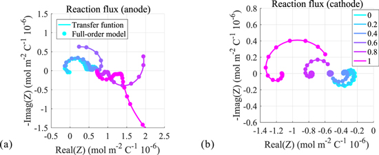
Figure 5. Frequency response of reaction flux.
Download figure:
Standard image High-resolution imageFrequency response of potential in the electrolyte
Nyquist plots of the electric potential in the electrolyte are shown in Fig. 6. This transfer function represents a proper impedance value as it comprises the ratio of a potential (that of the electrolyte) to the applied current. In the case of both electrodes, the dynamic is dominated by two clearly separated diffusion effects, indicated by the sequential first-order semicircles in each plot. Similar to that observed with the lithium concentration, we may again compute approximate dominant time constants by measuring the radial frequency at which the maximum imaginary part magnitude is attained. For the anode the time constants are well-separated; examination of the case for location 1.0 (electrode surface) gives a dominant time constant of  with a secondary (fast) time constant of
  Additional information may be gleaned from the real-axis intersection points of the Nyquist plot, which in this case can be associated with effective resistances to electron flow.
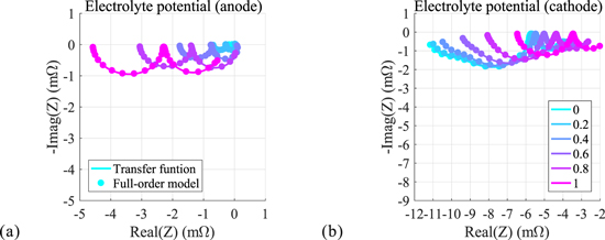
Figure 6. Frequency response of the electric potential in the electrolyte.
Download figure:
Standard image High-resolution imageFrequency response of potential in the solid
Nyquist plots of the electric potential in the solid are shown in Fig. 7. These responses may also be interpreted as true impedances for the corresponding electrodes and behave in similar fashion to cell impedance (to which they contribute). The basic form of the Nyquist plot for the anode again depicts first-order diffusion processes well-separated in time scale. The real axis intersection points further denote appropriate resistance values for electrode and electrolyte materials.

Figure 7. Frequency response of the electric potential in the solid.
Download figure:
Standard image High-resolution imageThe cathode exhibits similar behavior with the expected 180° phase shift. Note that both responses indicate significant variation of relative resistance values with location within the electrode.
Frequency response of the potential difference
Nyquist plots of the solid-electrolyte potential difference are shown in Fig. 8. The frequency response for the anode is very similar in form to the cell impedance obtained through EIS measurements. Regions corresponding to equilibrium capacitance (near-vertical portion), Warburg impedance (approximate 45° slope), and diffusion processes (semicircle) are clearly visible on the plot. It is of special significance that the frequency response of the potential difference (as well as other internal variables) is well-behaved in the sense that it turns out its generating components can be approximated by linear models of relatively low order. This has important implications for reduced-order modeling of these variables29 for use with advanced control strategies.

Figure 8. Frequency response of solid-electrolyte potential difference.
Download figure:
Standard image High-resolution imageFrequency response of the solid surface concentration
Nyquist plots of the solid-electrolyte potential difference are shown in Fig. 9. The solid surface concentration essentially reflects the charge behavior of the cell and is clearly dominated by the equilibrium capacitance which appears as the vertical line in both electrode plots. Diffusion processes are also captured, but are not easily visible at the scale.
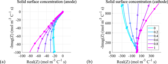
Figure 9. Frequency response of solid surface concentration.
Download figure:
Standard image High-resolution imageConclusions
In this Paper, we build the complete full-order model of porous-electrode lithium-ion cells by modeling the electrical double-layer in the solid-electrolyte interface and integrating it into the original P2D model. The electric double-layer model includes the resistance that lithium-ions need to overcome during the moving process, which makes the model more realistic. Using the Doyle–Fuller–Newman (DFN) cell parameters, we simulate the full-order model in the time domain. Then we obtain the cell impedance using a practical and straightforward identification method that calculates the impedance based on the input and output data in the time domain. This Paper also reveals and analyzes the frequency responses of internal electrochemical variables. From the results, we can see that even though the frequency-response models look quite complicated (mathematically), some fundamental frequency-response behaviors are relatively simple and can convey important underlying behaviors important to cell design. Additionally, the TF can be used to predict the behaviors of cell and internal electrochemical variables as an alternative to the full-order model.
In order to achieve the fast calculation of the cell impedance and internal electrochemical variable, this Paper describes in detail how to simplify and convert the full-order models into transfer functions, especially the transformation of the full-order model of the interfacial impedance. A method for obtaining the transfer function of cell impedance by the transfer function of internal electrochemical variables is also presented. The Nyquist plot results calculated by the transfer functions are exactly consistent with the results of the full-order models, which verifies the accuracy of the transfer function and the effectiveness of the simplified method. Furthermore, calculating cell impedance using the frequency-response method is on the order of 45,000,000 times faster than using direct simulation of the PDEs.
Acknowledgments
This research was supported by the National Natural Science Foundation of China (NSFC) under the Grant No. 51877138, the Shanghai Science and Technology Development Fund under the Grant No. 19QA1406200, and the China Scholarship Council (CSC) under the Grant No. 201808310186. This work used the EAS Data Center or EAS Cloud, which is supported by the College of Engineering and Applied Science at the University of Colorado Colorado Springs. We thank Dongliang Lu for valuable discussion.
: Appendix: Development of Transfer Functions
Once the transfer function for  has been derived, all other cell transfer functions can be found from it. The process for doing so is the same as derived in Rodríguez et al.,26 and the interested reader is referred to that reference for the detailed derivation. Here, we simply state the final results in an effort to make this Paper as self-contained as possible.
A.1. Coefficients of electrolyte-concentration transfer function
After quite a lot of tedious back-substitution, the coefficients  ,
,  ,
,  ,
,  ,
,  ,
,  ,
,  ,
,  ,
,  , and
, and  , of the electrolyte transfer function can be found exactly in closed form. The result from Rodríguez et al.26 applies exactly here, with the new definition of τ1(s) and τ2(s) and consequential modifications to the values of (but not equations for) quantities that depend on τ1(s) and τ2(s). The solution is expressed in terms of
where
for r ∈ {n, p}.
Then, the electrolyte-concentration transfer-function coefficients for the separator region are:
The coefficients for the negative-electrode region are:
The coefficients for the positive-electrode region are:
A.2. Reaction flux transfer function 

A transfer function for the total reaction flux in region r ∈ {n, p} is
where
Because there is no solid in the separator region, Js(z, s) = 0.
A.3. Solid–electrolyte potential difference transfer function


A.4. Solid surface concentration transfer function

Due to the addition of the enhanced solid/electrolyte interface description, the derivation of the transfer function for the solid surface concentration is somewhat different from in Rodríguez et al. We note that solid concentration is affected only by faradaic flux at the particle surface, not the double-layer flux (this is the same assumption made by Meyers et al.). Therefore, we can determine the solid-surface-concentration transfer function in a stepwise fashion for r ∈ {n, p}:
The first term is given in Eq. 30 and the third term has just been stated. However, the calculation of  depends on the exact interfacial model used.
For the default simplified model of Fig. 1c, we can write
A.5. Solid-potential transfer function

In the negative electrode, we define  . Then,
In the positive electrode, we define  . This gives
A.6. Electrolyte-potential transfer function
A.6.1. Negative electrode
We define the unbiased electrolyte potential as  . Then,
A.6.2. Separator region
In the separator,
A.6.3. Positive electrode
In the positive electrode,