

Abstract
The downtime of industrial machines, engines, or heavy equipment can lead to a direct loss of revenue. Accurate prediction of such failures using sensor data can prevent or reduce the downtime. With the availability of Internet of Things (IoT) technologies, it is possible to acquire the sensor data in real-time. Machine Learning and Deep Learning (DL) algorithms can then be used to predict the part and equipment failures, given enough historical data. DL algorithms have shown significant advances in problems where progress has eluded the practitioners and researchers for several decades. This paper reviews the DL algorithms used for predictive maintenance and presents a case study of engine failure prediction. We also discuss the current use of sensors in the industry and future opportunities for electrochemical sensors in predictive maintenance.
Export citation and abstract BibTeX RIS

This is an open access article distributed under the terms of the Creative Commons Attribution 4.0 License (CC BY, http://creativecommons.org/licenses/by/4.0/), which permits unrestricted reuse of the work in any medium, provided the original work is properly cited.
Sensors convert physical signals into electrical signals. This makes it possible to measure physical quantities in the environment. If such measurements are made repeatedly and stored, the behavior of the physical quantity can be studied. Further, if the data can be transmitted to the processing unit with minimal delay, a real-time analysis can be performed to gain valuable insights.
When an engine or heavy industrial equipment is operating, certain internal physical quantities such as oil temperature, oil pressure etc., change significantly. At the same time certain environmental variables such as external temperature and humidity also change. Analysing sensor data that captures these variables can reveal several things such as the health of the equipment and potential failures.
Engine and equipment failures are often associated with the internal or environmental variables exhibiting unexpected behavior. For example, the oil temperature going beyond the normal range can cause the engine to stop functioning. Continuous monitoring of such variables, predicting failures or degradation and taking actions to prevent them is referred to as Predictive Maintenance (PM).1 PM is one of the most important components of smart manufacturing and Industry 4.0. A recent report from "Allied Market Research" predicted that the market for PM will be worth $23 billion by 2026.2
The benefits of PM include reduced downtime, improved quality, reduction in revenue losses due to equipment damage, better compliance, reduced warranty costs and improved safety of operators. The most important goal of PM is to recognize uncommon system behavior and to have an early warning for catastrophic system damage.3–8
While diagnosis involves identifying the cause of an existing problem, prognosis is predicting the occurrence of a problem and its cause. In recent times, data-driven prognosis methods have proven to be very effective due to the availability of better data acquisition methods, Internet of Things (IoT) and Machine Learning (ML).9
ML offers algorithms that learn from data. The algorithms learn a representation of the training data, which is then used to make predictions on out-of-sample data. Deep Learning (DL) refers to a class of ML algorithms that use neural networks with several layers of processing units. Ref. 10 has discussed the importance of ML algorithms for electrochemical engineers. The emergence of DL algorithms has resulted in much better accuracy in prognosis. In this paper, we briefly explain the DL approaches for PM.11
In summary, the PM process involves data acquisition from various kinds of sensors, data transmission and storage, data pre-processing and then analysis. The analyzed data is used by the applications in the organization. A schematic of such a system is shown in Fig. 1.

Figure 1. A visualization of the system with data being collected from an industrial sensor network (based on IoT). The data is stored and managed on the cloud. The users can interact with the IoT devices from the command center. Data from the electrochemical, environmental and physical analyzed using neural networks to make predictions. Long term trends and analysis are depicted in a dashboard like application. The solid arrows indicate data flow. The dotted arrows indicate the contents of the element at the beginning of the arrow. The neural network depiction used here is taken from Command Center (CC) public domain.
Download figure:
Standard image High-resolution imageReview Methodology
The goal of this paper is to review DL methods that are applicable to sensor data in the context of PM. It is not an exhaustive survey of all DL methods but the ones that are relevant to this domain and the most effective.
The language used to refer to Industrial IoT is not consistent throughout the world. Also, there are several types of sensors, various types of analysis required for prognosis and a lot of DL algorithms to choose from. For this research, we first created a table of keywords as mentioned in Table I. Several combinations of the keywords from each column of Table I were used to search in Google Scholar and Web of Science. An example search phrase constructed this way is, "Anomaly Detection using LSTM for Equipment Health Monitoring". From the results obtained, relevant papers were selected, giving priority to peer-reviewed journals and papers with more than 10 citations. Since DL gained momentum after 2012, a significant portion of the chosen papers are from the last five years.
Table I. Keyword combinations used for literature search.
| Data Source | Type of Analysis | Algorithm | Application Keywords |
|---|---|---|---|
| Electrochemical sensors | Prediction | Deep learning | Predictive maintenance |
| Environmental sensors | Anomaly detection | Neural networks | Smart manufacturing |
| Physical sensors | Prognostics | CNN | Industry 4.0 |
| Acoustic sensors | Forecasting | RNN | Industrial IoT |
| Electric sensors | Remaining useful life | LSTM | Health monitoring |
| Image sensors | Trend analysis | Autoencoder |
Sensors in the Industry
In recent years, there has been an increase in the number of electrochemical and optical sensors in various industrial applications (i.e. health/medicine, automotive, food safety, environmental monitoring, and agriculture). In the case of industrial/plant settings, the applications of these sensors have found to be ubiquitous. For example, Ref. 12 has developed a hydrogen peroxide sensor using gold-cerium oxide which has applications in oil and petrochemical refineries. Reference 13 also used Au based electrodes to monitor ammonia in diesel exhaust. The sensor construct was later transitioned to a pre-commercial, automotive stick sensor configuration which performed comparably to prior tape-cast sensor devices. Reference 14 demonstrated the use of zirconia-based mixed potential electrochemical hydrogen gas sensors for safety monitoring in commercial California hydrogen filling stations. The performance of the developed sensors showed a high sensitivity to hydrogen and fast response times.
Electrochemical sensors are also common in food safety, agricultural and environmental monitoring fields. Reference 15 developed an electrochemical sensor based on nanocomposite materials to detect gallic acid in food samples. The sensor showed high sensitivity in real sample analysis. In Ref. 16, a Cu deposited Ti electrode was used to monitor excess nitrate accumulation in slow-flowing water bodies. High nitrate concentrations in surface waters are a precursor to algal blooms and eutrophication. The sensor showed to be highly sensitive, reliable and stable in wide pH ranges. Screen-printed electrodes (SPEs) were used in Refs. 17, 18 and 19 to monitor caffeine, Ca2+, and toxic mercury in surface and sewage waters. The SPE developed by Ref. 17 was based on a thin bismuth film layer that facilitated a diffusion-controlled process of the electrochemical oxidation of caffeine. The overall performance of the sensor showed both good selectivity and good agreement to the results obtained by reference to high-performance chromatography. The SPE fabricated by Ref. 18 was based on an all-solid-state Ca2+-selective polymeric membrane indicator electrode. The sensor proved to be an alternative tool for on-site and rapid detection of Ca2+ for marine monitoring. Reference 19 described a facile synthesis of tungsten carbide nanosheets (WC NSs) for monitoring trace levels of toxic mercury ions in biological and contaminated sewage water. The modified SPE attained a detection limit well below the guideline set by the U.S. Environmental Protection Agency (EPA) and the World's Health Organization (WHO). The results obtained from the industrial wastewater samples were found to be comparable to standard techniques.
In addition to the many types of electrochemical and solid-state sensors, optics-based sensors have also found their use in industrial and environmental monitoring. Reference 20 reviews Surface-Enhanced Raman Scattering (SERS) sensors that can be used for the detection of heavy metals, among other applications. And Ref. 21 has presented the dangers of heavy metal toxicity in industrial effluents. Hence there is a potential application of SERS sensors in monitoring industrial waste.
Continuous monitoring
IoT can be used to continuously acquire sensor data and interact with the environment.22 This has been demonstrated by Refs. 23–25 and 26. Our research group has demonstrated the use of electrochemical sensors for continuous monitoring of bio-signals in Refs. 23 and 24 respectively. Reference 23 developed and tested a miniaturized wearable fuel cell sensor that can detect isoflurane gas vapors in the therapeutic ranges. The IoT device is interfaced with a Bluetooth radio module and incorporated into a life support system for casualty evacuation with autonomous UAV emergency medical operations. Reference 24 developed a platform for monitoring wound healing and management. The miniaturized flexible platform was based on a wearable enzymatic uric acid biosensor interfaced with a wireless potentiostat. These examples demonstrate the use of electrochemical sensors for continuous monitoring.
Reference 25 also developed IoT sensor sheets to help everyday home and commercial gardeners reduce excessive fertilizer application. The nitrate sensing platform functions by using wireless potentiometry to monitor leached nitrate from south Florida garden soils in real-time. Reference 26 also utilized an IoT sensor network approach to smart farming. The real-time sensor network, which consisted of soil moisture sensors, solar radiation sensor, soil temperature, leaf wetness sensors, and a weather station, offered insight on the nexus between the food, energy, and water resources and crop yield for several essential crops.
In addition, oxygen sensors, which are electrochemical in nature,27,28 have been used in the automotive industry for a long time and are also being used in IoT data acquisition.
The vision of Industry 4.0 involves collecting data from sensors, machines, and tools connected through IoT. The processing of the data can happen either on the device or centrally.
There is also an uptick in the application of artificial intelligence (AI) with sensor data. For example, The researchers in Ref. 29 have achieved water quality monitoring using AI (conclusion and findings). The data from the embedded electrochemical and optic-based sensors can be used for anomaly detection, defect localization, prognostics, forecasting, diagnosis, optimization, and control in industrial applications.1 Table II provides examples of sensors and their potential use in the industry.
Table II. Examples of electrochemical sensors in the industry. Some of the sensors are already suitable for Industrial IoT applications but the others have a future potential.
| Example | Sensor type | Potential use or industry |
|---|---|---|
| Corrosion sensors30 | Optical color sensors with electrochemically active compounds | Aircraft and heavy equipment maintenance |
| Hydrogen peroxide sensor12 | Gold-cerium oxide | Oil and petroleum industry |
| Heavy metal sensors20 | SERS | Monitoring industrial effluents |
| Oxygen sensors28 | Potentiometric sensors based on zirconia | Diagnostics/Prognostics in automotive industry |
| Nitrate sensor16 | Cu-Ti electrode | Environmental monitoring |
| Nitrate leachate sensor25 | N-doped PPy ISE | Agriculture |
| Caffeine sensor17 | BiF/SPCE | Environmental water monitoring |
| Ca2+ sensor18 | Solid state ISE | Environmental water monitoring |
| Hg (II) sensor19 | WC NSs | Environmental sewage water |
| Isoflurane gas sensor23 | Wearable fuel cell | Medical/Health |
| Uric acid sensor24 | Enzymatic biosensor | Medical/Health |
| Gallic acid sensor15 | Nanocomposite materials NiAl2O4 | Food safety |
| Ammonia sensor13 | Au and Pt + YSZ | Automotive/Diesel exhaust monitoring |
| Hydrogen sensor14 | Zirconia based electrode | Fueling station safety |
Sensor Data Analysis and ML
The variables of interest can vary with space or time. And the collected data is referred to as spatial and time-series data respectively. Examples of variables that constitute time-series data are temperature, pressure or concentration of a chemical such as uric acid. An example of spatial data is images from optical sensors. Table III presents the learning methodology and the deep learning architecture for various tasks.
Table III. Choosing a DL architecture.
| Task | Type of learning | Deep learning architecture |
|---|---|---|
| Denoising | Unsupervised | Auto-encoders |
| Dimensionality Reduction | Unsupervised | Auto-encoders |
| Forecasting future sensor output | Supervised | ANN/RNN/CNN |
| Anomaly Detection | Supervised/Unsupervised/Semi-supervised | RNN/Auto-encoders |
| Detection of structural damage | Supervised | CNN |
| Pre-training the network | Unsupervised | Autoencoders |
For PM, data from several sensors is acquired and hence the data is referred to as multi-variate time series data. In some applications, data from thousands of sensors is collected for analysis. If the number of independent variables in the data is very high it is referred to as high dimensional. Before an ML algorithm is applied to the sensor data, it is important to ensure that it is in the right format or structure. This is referred to as pre-processing.
Pre-processing can involve steps such as denoising and dimensionality reduction. Denoising refers to eliminating noise from a signal to improve the signal-to-noise ratio. Dimensionality reduction refers to reducing the number of independent variables in the data while minimizing the loss of information. ML and DL can help in pre-processing as well. Specific statistical and ML algorithms used in dimensionality reduction can be found in Ref. 31. Autoencoders are specific variants of DL neural networks that can be applied to denoising or dimensionality reduction.32
Anomalies in data can indicate a fault that has already occurred or a potential fault. There are several approaches to finding anomalies in data, but we focus on two of them, where DL is applicable. One approach to finding anomalies is to use the time-series sensor data to predict subsequent values and compare the deviation against a set threshold. For this approach, both Recurrent Neural Networks (RNNs), as well as Convolutional Neural Networks (CNNs), can be used. The second approach is to use a neural network to learn a representation of the data and then reconstruct it. A comparison of the actual values with the reconstructed values gives the reconstruction error. If the reconstruction error is more than a set threshold, it can indicate an anomaly. Autoencoders are suitable for the second approach.33–36 A thorough discussion on anomaly and outlier detection methods can be found in Ref. 37. Figure 2 presents the top-level block diagram of the data analysis pipeline.

Figure 2. A visualization of the data analysis pipeline. The sensor data is acquired and stored in a database. This is followed by pre-processing and model building. The end goals of the analysis include but not limited to failure prediction, anomaly detection and Remaining Useful Life (RUL) analysis.
Download figure:
Standard image High-resolution imagePrognostics is the prediction of a future problem, forecasting is the prediction of a future sensor value, and Remaining Useful Life (RUL) analysis is the estimation of the duration after which the operating point of the sensor drifts to an undesired region.38 All these PM tasks involve predicting the future values of a sensor. ML and DL algorithms are effective for the prediction and regression tasks.
Supervised learning
Supervised learning is the most frequently used type of ML. In this type of learning, training samples are accompanied by target variables, which are also called labels. The data in this case can be represented as shown in Eq. 1,39 which represents a set of ordered pairs. xi represents a vector of independent variables and yi represents the value of the dependent variable for the ith sample. N represents the number of data samples.

xi can be numbers, audio or images based on the sensor being used. ML attempts to learn representations of the data that is useful in making predictions. The learning process involves finding the optimum values of the parameters that constitute the representation, called model, in order to minimize the loss function. Equation 2 shows an example loss function, which is Mean Squared Error (MSE). The choice of the function depends on the specific problem being solved.

The loss function is an estimate of the overall error in the relationship learned by the model. The error for each training sample is the difference between the actual and predicted values.
Unsupervised learning
ML approaches applied when the target data or annotated training labels are not available is called unsupervised learning. The data in this case can be represented as shown in Eq. 3.39 The representation is similar to Eq. 1, where xi represents a vector of independent variables for the ith sample, but values of yi are not available.

Clustering, dimensionality reduction and denoising are examples of unsupervised tasks. Since there is no target data, which provides reference values for learning, unsupervised learning is very challenging. It is an active research area.
Deep Learning Methods
Neural networks (feed-forward) are efficient in functional approximation of the type y = f(x)40 where x is the input and y is the target variable. In the case of PM, neural networks can be used to find the relationship between the features (independent variables), that come from sensor values, and the dependant variable(s). The dependant variable can be the time of failure, future sensor value or the presence of an anomaly. The goal of a feed-forward neural network is to learn the parameters θ, shown in Eq. 4 as per the mapping f. Each feature vector is made up of data from one of the sensors. The term "feed-forward" is used to indicate that the information moves from the input x to to the output y.40


Deep neural networks consist of layers of connected processing units. Each layer learns a representation of the data and together the network learns a complex function as a chained sequence of sub-functions. Equation (5) represents a network with three connected layers. fi corresponds to the ith layer. The term "deep learning" refers to the hierarchical representations of data using multiple layers of processing units.
Each of the layers has parameters or weights that are learned during the training process, similar to θ in Eq. 4. DL uses the backpropagation algorithm to update the parameters in each of the processing layers during the learning process. For more information on backpropagation, refer to Refs. 11 and 40.
Weights of the network are initialized with small random values. For every training sample, predictions are made based on the existing weights and the output is compared to the target value or label. An objective function (similar to Eq. 2) is used to make this comparison and calculate an error value. The error value is fed to an optimizer that updates the network weights accordingly. One pass of all the training samples through the network is called an "epoch". And the training continues for the user-specified number of epochs or until the desired reduction in error is achieved.4,11
The architecture of the neural network, including the activation function in each layer, is chosen and optimized as per the problem being solved. The user also chooses the optimizer and the objective function as per the needs of the dataset and the problem.
DL can involve learning thousands of weights and may need hundreds of thousands of training samples to achieve the desired accuracy. Industrial IoT sensors produce large volumes of data and hence suitable for applying DL. Electrochemical or solid state sensor systems should be designed to be able to support a high sampling rate.
Artificial neural networks
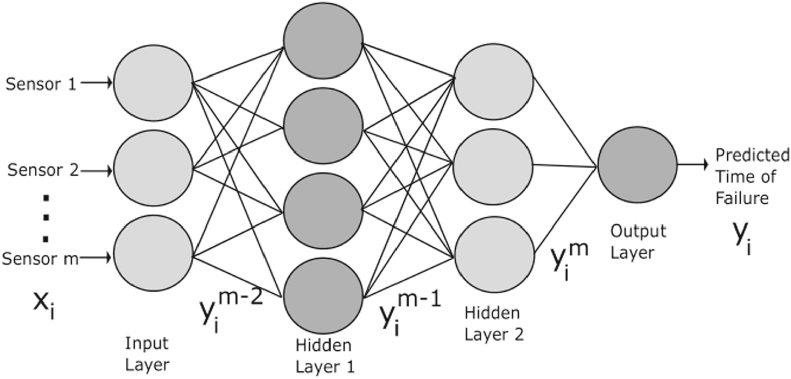
The processing units in each layer of an Artificial Neural Network (ANN), referred to as nodes, are connected to all the nodes in the next layer and are known as a fully connected layers.41,42 ANNs are commonly used for function approximation and pattern recognition purposes using supervised learning.43 They are therefore well suited for forecasting and prognosis. ANNs consists of an input layer, an output layer and one or more hidden layers as shown in Fig. 3.


Figure 3. A simple ANN with two hidden layers. The input is multivariate data coming from various sensors, including the timestamps. The output is the predicted time of failure for the engine.
Download figure:
Standard image High-resolution imageEquations 6 and 7 are used to calculate the output of the mth layer of the ANN shown in Fig. 3.40 The number of nodes in the mth layer are Nhm. The weight and bias of the mth layer are given by Wi,jm and bjm. In Eq. 7, the function A represents the activation function.
Convolutional Neural Networks (CNN)
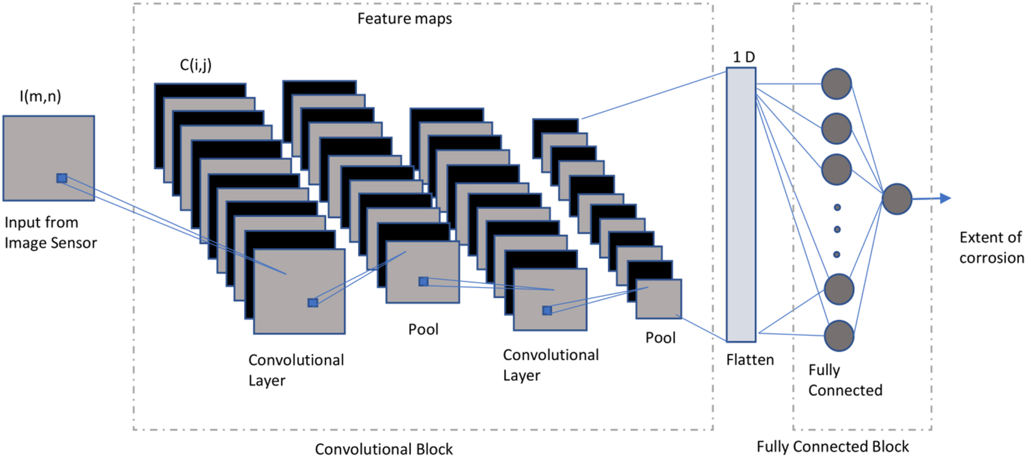
A network layer that uses the convolution operation is referred to as a convolutional layer. Figure 4 shows a representative image of a CNN applied to two dimensional sensor data. CNNs can also be applied to one dimensional sensor data. There are two parts in the CNN architecture. The first part consists of convolutional and pooling layers, that helps to extract features from the input data and the second part (fully connected layers) learns a representation of the training data to predict the target variables.11,44

Figure 4. A CNN with 2 convolutional layers interspersed with pooling layers. The network can be seen having two important blocks, the convolutional block and the fully connected block. The output from the convolutional block is flattened and used as input to the fully connected layers.
Download figure:
Standard image High-resolution imageThe discrete convolution operation is used to learn local patterns in data, either 1D or 2D, using a learnable filter. If the input and filter are denoted by I and K respectively, then the output of the convolution operation C is given by Eq. 8. The network in Fig. 4 uses two convolutional layers. The output of each convolutional layer is referred to as the feature map.45–47

Pooling operation is a way of down-sampling that decreases the number of features and reduces overfitting. Before being fed into the fully connected layers, the feature map is flattened into a 1D array.
Recurrent neural networks
The Recurrent Neural Networks (RNN) is a generalization of neural networks to learn sequences.48 RNNs can easily map sequences into a single output or sequential output.49,50 They are networks with loops that allow information to persist. Figure 5 shows the loop architecture and visualizes the unrolled RNN. Xt represents the input and ht represents the output at the current state. RNN contains several instances of the same nodes, where the output of one is fed as the input to the successive node. RNNs have the ability to handle sequences of various lengths. PM data consists of time-series and can have input samples of various lengths.


Figure 5. Visualizing a simple RNN unit and unrolled RNN unit. St−2, St−1 and st are state vectors that are passed on to the next time instance. The weight vector W is common to all the time steps.
Download figure:
Standard image High-resolution imageEquation 9 represents a dynamic system,40 which is a system with memory. h(t) is the output at time t, and depends on the input x(t) and the previous output at t − 1, which is h(t−1). The output also depends on θ which represents the learned weights. Equation 10, which is equivalent to Eq. 9, shows how the output at time t depends on all the previous inputs. Infact, Fig. 5 is a visualization of these equations.
Long Short-Term Memory (LSTM) networks are a special type of RNN with a capability of long-term dependencies which would be essential for our dataset. LSTM will help us look back for long periods before prediction. LSTMs will also help us extract and identify features from the sensor data that are essential for prediction. For a thorough discussion on LSTM please refer to the seminal paper that introduced it.51
Autoencoders
An autoencoder is a unique neural network with a goal of learning a representation that closely replicates the inputs as the output. The autoencoder has two parts, the encoder and the decoder as shown in Fig. 6. The input and output layers have the same number of nodes and all the layers are fully connected, but the network introduces a bottleneck in order to force the network to learn only the essential features. The bottleneck is introduced by choosing the number of nodes in the connecting layer, between encoder part and the decoder part, to be less than the number in the input layer. The training process is similar to other neural networks, where the weights and bias of the network are learned while minimizing a loss function.52

Figure 6. A simple autoencoder with only one hidden layer. The number of nodes in the hidden layer need to be less than the input layer to create a bottleneck. The input itself is used as the target data and hence the same number of nodes in the input and the output layers.
Download figure:
Standard image High-resolution image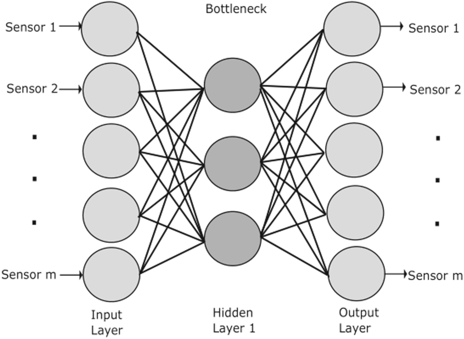
The encoder learns a representation of the input data and the decoder reconstructs the input from the learned representation. This process of learning and reconstruction is leveraged for various purposes. Denoising and dimensionality reduction are applications that are relevant to PM. Denoising can help in improving the quality of data and hence the quality of the forecasts. Dimensionality reduction can help improve computational efficiency when the data is high dimensional.53–55
Choosing a network
Forecasting and prognosis are usually implemented using supervised learning. For time-series data, the sensor values themselves constitute the target values. A sliding window is used to form sequences and the sensor value immediately next to the window is the target value for each position of the window.56
Anomaly detection can be supervised or unsupervised. When annotated historical data is available with both normal and anomalous samples, supervised learning can be applied. In several cases, there is no annotated data available, and unsupervised learning is the only option.
There are several variations of CNN, RNN, and autoencoders that have not been discussed in this paper. For more details refer to Refs. 57 and 58. In addition, there are training techniques such as transfer learning, that are also out of scope for this paper. For more details refer to Refs. 44, 59, 60.
Literature Review
ANN
ANNs have been used for PM for several years. For example, Refs. 61, 62 and 63 used ANN for fault diagnosis in motor rolling bearing fault diagnosis and Ref. 63 has demonstrated the use of neural networks for machine condition monitoring. Several researchers have demonstrated the effectiveness of using neural networks for system monitoring and prognosis.
The work referenced in this subsection demonstrates that the specific applications for neural networks in PM were identified and demonstrated in the prior decades. The work done since 2012 has been focused on applying the variants of DL neural networks such as CNN, RNN, etc., which improved the accuracy of the predictions based on the data. A case study presented later in this Paper, shows the improvements in accuracy and precision by using DL methods.
CNN
Sensor data from industrial and automotive equipment can be 2D or 1D. The right variant of CNN is chosen as per the available data. References 64–66 used 2D CNNs for fault detection and Ref. 67 used it for fault diagnosis. Reference 45 has used 1D CNN for fault diagnosis and Ref. 68 has used 1D CNN for fault detection.
CNN also has applications in RUL and structural damage detection. Reference 69 used CNN for RUL. Reference 46 has used 1D CNN for structural damage detection using data from vibrational sensors. CNNs are highly suited for images and may be used for the analysis of image sensor data analysis.
RNN
RNN based architectures are well suited for sequence learning and hence used extensively in time series forecasting. Prognostics and RUL are direct applications of predicting future values of time-series sensor data. Reference 70 used LSTM for fault diagnosis and Ref. 7 1 for RUL estimation. Reference 71 used LSTM for forecasting and prognostics. Fault diagnosis is achieved by predicting future sensor values and comparing them with actual values. If the deviation is very high, it can be an indicator of an underlying problem or a direct fault. Table IV presents the brief summary of DL methods applied to PM using sensor data.
Table IV. DL methods for PM using sensor data.
| References | Sensor data | Type of network | Application |
|---|---|---|---|
| 61 | Vibration sensors (ring and triaxial accelerometer) | ANN | Fault Diagnosis of rolling element bearings |
| 63 | Vibration sensors | ANN | Fault diagnosis and machine condition monitoring of induction motors |
| 64 and 65 | Frequency spectrum extracted from vibration sensor data | 2D CNN | Fault detection in rotating machines and gearbox |
| 67 | Vibration data from Input and output shaft | 2D CNN | Small fault diagnosis |
| 45 and 68 | Vibration sensor data | 1D CNN | Fault diagnosis |
| 69 | Frequency spectrum of Vibration sensor data | 2D CNN | RUL Estimation |
| 46 | Vibration sensor data | 1D CNN | Structural damage detection |
| 70 | Multimodal data with 58 sensors on the engine such as temperature and pressure etc | LSTM—RNN | Fault diagnosis and RUL estimation of aero engines |
| 72 | Frequency spectra from vibration sensors | LSTM—RNN | RUL Estimation of rotating machinery |
| 71 | Dynamometer, accelerometer and acoustic sensors | LSTM—RNN | Forecasting and prognosis of milling machines |
| 33 | Multimodal data with ambient temperature sensor, motor temperature sensor, load and current data | Autoencoder | Fault diagnosis |
| 73 | Acoustic sensor data | Autoencoder | Fault diagnosis in rolling bearings |
| 74 and 75 | Vibration signals | Autoencoder | Motor fault classification |
| 76 | Acoustic sensor data | Autoencoder | Anomaly detection in air compressors |
| 36 | Temperature sensors | Autoencoder | Anomaly detection in gas turbines |
| 38 | Multimodal sensor data from a turbofan engine | LSTM based Autoencoder | Sensor data forecasting for RUL |
Autoencoders
Reference 55 has demonstrated the effectiveness of denoising autoencoders in 2008. Post-2012, with more focus on DL based methods, several other researchers applied autoencoders for fault detection, fault classification, and denoising. References 77–79 used autoencoders to pre-train the neural network and then fine-tune it using the backpropagation algorithm. The underlying approach is to first use unsupervised learning to learn a representation of the data and then fine-tune it using supervised learning. References 33, 73, 80 also used autoencoders for fault diagnosis. References 74, 75 used a similar approach and applied autoencoders for induction motor faults classification.
Autoencoders are highly effective in anomaly detection. References 76 and 36 have successfully used autoencoders for anomaly detection. This approach includes learning a representation of the data and reconstructing the data. An exceptionally high error in reconstruction is an indicator of an outlier or an anomaly. Reference 56 used a semi-supervised approach for failure prediction. Among all the DL architectures, the autoencoders have been used for more PM tasks compared to other variants. LSTM nodes can also be used to build autoencoders. Such autoencoders are very well suited for sequential data. Reference 38 used an LSTM based autoencoder for sensor data forecasting.
Case study
The sensors group at Florida International University in collaboration with the sensors and systems group at University of Dayton Research Institute studied PM using ML and tested various approaches on a publicly available dataset.
The dataset used in the project was made available public by Ref. 81. The dataset consists of data from 21 sensors on a turbofan aircraft engine. The data was extracted under simulated engine degradation conditions. The researchers simulated four different sets under various conditions to create several fault modes. They also captured data from several sensors to study the fault evolution. This dataset is part of a NASA's prognostics data repository.
The various sensors used include, temperature sensors, pressure sensors and sensors to measure fan speed, fuel-air ratio, and coolant bleed. Please refer to Table III in Ref. 82 for more detailed descriptions of the sensors.
The focus of the project is to predict a machine's failures well in advance and take appropriate action. In the template provided on the website, three modeling solutions were studied: regression-based model to predict the RUL and Time to Failure (TTF), binary classification model in order to classify if an asset will fail within a particular time frame and a multi-class classification model to predict if an asset will fail in different time frames.
We utilize the same set of training, validation and testing data as provided in Ref. 81 summarized in Table V. The data consists of multi-variate time series with the cycle as the time unit. Each cycle comprises 21 sensor readings which essentially serves as features (or independent variables) for our ML algorithm. Each time-series is assumed as being generated from a different engine of the same type. The last cycle in each time-series is considered as the failure point for the respective engine during the training process. While testing, we utilize the truth data provided along with the testing data in order to estimate our performance. The focus is on solving this problem as a classification task where the labels are determined as described in the database81 with TTF values at a threshold of 30. The distribution of dataset is as shown in Table V.
Table V. Training and testing dataset composition.
| Dataset | #Non-defective | #Defective |
|---|---|---|
| Training | 17631 | 3000 |
| Testing | 12789 | 307 |
Various methods for determining the probability of aircraft engine failing within a cycle were researched and studied. All the data points are converted into a time-series (with a window length of 50). Each time-series is generated from a different engine of the same type. Traditional ML methods are developed solely based on features which do not consider past values for predictions thus making it harder.
Sensor values of 50 cycles prior to the failure of each engine (engines are distinguished by id) are extracted. Note that the sequences are not padded, and the sequences that do not meet window length of 50 are not considered for the study. This type of pre-processing is implemented for both training and testing dataset.38,70,71,83–85
A total of five algorithms are implemented and tested. The traditional ML algorithms used are, Logistic Regression (LR), Support Vector Machines (SVMs) and an Ensemble Model. A fully connected neural network (ANN) is also implemented. And finally, an LSTM network as described in the previous Section is applied to the dataset. The results are summarized in Table VI. For more details about SVM, ensemble models and LR, refer to Refs. 3, 86 and 87 respectively.
Table VI. Comparing the performance of various algorithms.
| Algorithm | Area under the curve | Precision |
|---|---|---|
| Logistic Regression | 0.990 3 | 0.596 |
| Fully connected Neural Network | 0.990 2 | 0.629 |
| SVM | 0.990 2 | 0.593 |
| Ensemble model | 0.988 6 | 0.775 |
| LSTM | 0.998 | 0.873 |
The overall accuracy is the ratio of the number of predictions that are right to the total number of predictions. LSTM achieved an accuracy of 99.3%. Also, the Receiver Operating Characteristic (ROC) curve is a graph of the True Positive (TP) rate vs the False Positive (FP) rate. The Area Under the ROC Curve (AUC) is a quantitative measure of the performance of the model. AUC varies from 0 to 1, with 1 being the ideal scenario. The AUC achieved with LSTM is 0.998. From Table VI, it can be noticed that all the ML algorithms that is tested show good performance as per the AUC.88
The LSTM model is found to be more effective compared to the other models for this dataset. Even though there is minimal difference in AUC values for all the models, there is a striking difference in terms of the precision score. LSTM is able to detect 268 out of the 307 faults, thereby achieving a high precision score of 87.3%. This demonstrates the superiority of LSTM, when learning from sequential data. Table VI shows the precision scores of all the algorithms.
Conclusion and Future Perspectives for Electrochemical Sensors
Industrial IoT is one of the fastest-growing segments of modern data deluge. Sensors form the backbone of this revolution. The goal of deploying these sensors and acquiring data is to analyze it for insights. The right insights at the right time, about the industrial or automotive equipment, can help the technicians or engineers take preventive action. Recent progress in ML and DL algorithms, the availability of the right sensors and ubiquitous computational power enables automated predictive maintenance.
Data-driven methods and ML algorithms have been around for several years. But in recent times, DL algorithms have made tremendous strides in performance and have improved the state of the art in predictive maintenance. Hence, DL architectures for predictive maintenance are the focus of this paper.
This paper has reviewed the use of sensors in the industry with several examples of electrochemical and solid state sensors. This paper has also reviewed the DL algorithms which can be applied to the data coming from these sensors. It can be expected that there will be an increase in the use of data from electrochemical and solid state sensors for predictive maintenance.
A hypothetical example includes an agricultural sensor for determining water quality. A typical predictive maintenance situation would include the original data derived from the target sensor plus the additional sensor data from surrounding environments which might influence degradation of the target sensor (i.e. temperature, moisture, pressure, pH, and additional metals and ions). Over a given time we would expect to experience a deviation from actual measurements, or sensor drift. Predictive maintenance can use the surrounding data to ensure that drift will not occur, or it can use the drift as an indication to perform maintenance.
Design considerations of chemical sensors for future applications in DL should include a system which supports high sampling rates. Given the amount of large data required for ML and DL applications, the future sensor designs should consider repeatability in measurements, long lifetime, and also include a self re-calibrating system for correcting sensor drift. In addition, all of the standard considerations for characterizing sensor analytical performance are of great importance, although this also depends on the target being analysed and the functional material of the sensor system.
Acknowledgments
We would like to thank NASA AMES Research Center for making data available to public. We also thank the anonymous reviewers for their help in strengthening this paper.